Visual orbit for the low-mass binary Gliese 22 AC from speckle interferometry

Based on 14 data points obtained with near-infrared speckle interferometry and covering an almost entire revolution, we present a first visual orbit for the low-mass binary system Gliese 22 AC. The quality of the orbit is largely improved with respect to previous astrometric solutions. The dynamical system mass is $0.592\pm 0.065\,M_{\sun}$, where the largest part of the error is due to the Hipparcos parallax. A comparison of this dynamical mass with mass-luminosity relations on the lower main sequence and theoretical evolutionary models for low-mass objects shows that both probably underestimate the masses of M dwarfs. A mass estimate for the companion Gliese 22 C indicates that this object is a very low-mass star with a mass close to the hydrogen burning mass limit.

1 Introduction

M dwarfs are the dominant population of the Galaxy as well in numbers as in stellar mass contribution. Furthermore, they mark the transition regime between stars and the now well established classes of substellar objects. Given these important properties, it is problematic that there is only a small number of empirically determined stellar masses at the lower end of the main sequence. In addition, most of these dynamical masses are affected with large uncertainties (e. g. Henry Hen98 (1998)). This means that the mass-luminosity relation for M dwarfs is not well calibrated. Moreover, theoretical evolutionary models for low-mass objects that cover also the substellar regime are not well checked with dynamical masses.
As a contribution to a solution of these problems we are carrying out a program aiming at a determination of visual orbits and thus dynamical masses for M dwarf binaries. Speckle interferometry with array cameras in the near infrared allows highly precise measurements of the relative astrometry in sub-arcsecond binary or triple systems.
This program has already led to orbit determinations for the very low-mass systems Gliese~866 (Woitas et al. Woi00 (2000)) and LHS~1070 BC (Leinert et al. Lei01 (2001)). The companions in these systems appear to have masses close to the stellar/substellar limit at $M\approx 0.075\,M_{\odot}$. In this paper we discuss a first visual orbit determination for Gliese~22 AC that was briefly announced in IAU Commission 26 Information Circular 147 (Docobo et al. Doc02 (2002)).
A visual companion to the M2 star Gliese 22 (other designations: HIP 2552, BD +66$^∘$34, ADS 440, V~547~Cas) was first reported by Espin & Milburn (Esp26 (1926)). At the time of this detection the projected separation was 2$\aas@@fstack{\prime\prime}$79. The orbital motion of this companion with a period of $\approx 320$ yr has been monitored since its detection, and most recent orbital elements are given by Lampens & Strigachev (Lam01 (2001)). Alden (Ald47 (1947)) found that the primary component of this pair is itself an astrometric binary. Herafter, we will refer to this close pair as Gliese 22 AC and to the more distant third component as Gliese 22 B. Hershey (Her73 (1973)) presented orbital elements for Gliese 22 AC based on a rich collection of astrometric plates from the Sproul Observatory. This calculation was refined by Heintz (Hei93 (1993)) adding more data points and Söderhjelm (Sod99 (1999)) including the Hipparcos parallax of Gliese 22 into the analysis.The first two resolved visual observations of Gliese 22 AC were reported by McCarthy et al. (Mcc91 (1991)) using near-infrared speckle interferometry. Since the epoch of these first two measurements we regularly observed this pair obtaining 12 more data points, which uniformly cover almost an entire revolution. Based on these data, we present in this paper a visual orbit and a dynamical system mass that are more precise than the previous astrometric solutions. We will describe the techniques of observations and data analysis in Sect. 2 and present the result of the orbit calculation in Sect. 3. In Sect. 4 we will discuss implications of the derived dynamical system mass on the mass-luminosity relation and theoretical models for very low-mass objects.

2 Observations and Data Analysis

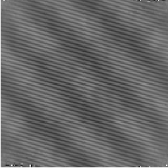
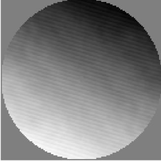
Figure 1: Modulus (left) and bispectrum-phase (right) for Gliese 22, derived from 1000 short ($\tau=0.2\,\mathrm{s}$) exposures obtained at $\lambda=2.2\,\mu\mathrm{m}$ with OMEGA Cass at the 3.5-m telescope on Calar Alto on 3 November 2001. North is to the top and east to the left. The broad stripe pattern in the modulus is due to Gliese 22 AC while the fine patterns (roughly from top to bottom) are produced by the more distant companion Gliese 22 B. The phase has been cut off at the Nyquist frequency that is 5.3 arcsec^-1 for the adopted pixel scale of 0$\aas@@fstack{\prime\prime}$095/pixel.

Table 1: Overview of all observations of Gliese 22 AC used for the visual orbit determination in this paper. Except for the first two data points all observations have been carried out at the 3.5-m telescope on Calar Alto.

No.	Date	Epoch	Position angle	Projected	Weight	Filter	Flux ratio	Instrument
			angle [∘]	separation [mas]			$F_{C}/F_{A}$	(or reference)
1	12.10.1989	1989.7803	42.7 $\pm$ 2.5	451 $\pm$ 20	4	K	0.167 $\pm$ 0.009	McCarthy et al. Mcc91 (1991)
2	10.12.1989	1989.9418	43.9 $\pm$ 2.5	453 $\pm$ 20	4	H	0.143 $\pm$ 0.008	McCarthy et al. Mcc91 (1991)
3	11.09.1990	1990.6954	57.1 $\pm$ 6.3	405 $\pm$ 39	5	K		1D
4	20.09.1991	1991.7201	71.6 $\pm$ 1.6	443 $\pm$ 13	5	K		1D
5	30.09.1993	1993.7474	122.5 $\pm$ 0.5	464 $\pm$ 11	7	K	0.151 $\pm$ 0.004	MAGIC
6	28.01.1994	1994.0767	129.3 $\pm$ 4.3	478 $\pm$ 40	10	K		MAGIC
7	15.09.1994	1994.7064	141.1 $\pm$ 0.4	510 $\pm$ 5	9	K	0.141 $\pm$ 0.007	MAGIC
8	13.12.1994	1994.9501	145.2 $\pm$ 0.2	532 $\pm$ 5	9	K		MAGIC
9	08.10.1995	1995.7693	157.5 $\pm$ 1.7	526 $\pm$ 16	9	K	0.158 $\pm$ 0.004	MAGIC
10	28.09.1996	1996.7448	172.1 $\pm$ 0.2	533 $\pm$ 4	10	K	0.141 $\pm$ 0.004	MAGIC
11	17.11.1997	1997.8789	190.2 $\pm$ 0.3	460 $\pm$ 4	7	K	0.171 $\pm$ 0.008	MAGIC
12	09.02.2001	2001.1095	302.3 $\pm$ 0.3	334 $\pm$ 4	9	K	0.185 $\pm$ 0.005	OMEGA Cass
13	03.11.2001	2001.8406	325.5 $\pm$ 0.5	402 $\pm$ 6	8	K	0.151 $\pm$ 0.011	OMEGA Cass
14	19.10.2002	2002.7994	348.2 $\pm$ 0.4	463 $\pm$ 5	9	K	0.150 $\pm$ 0.005	OMEGA Cass

Table 2: New observations of the wide pair Gliese 22 AB obtained at the 3.5-m telescope on Calar Alto.

No.	Date	Epoch	Position angle	Projected	Filter	Flux ratio	Instrument
			angle [∘]	separation		$F_{B}/F_{A}$
1	30.09.1993	1993.7474	164.4 $\pm$ 0.5	$4\aas@@fstack{\prime\prime}24\pm 0\aas@@fstack{\prime\prime}09$	K	0.199 $\pm$ 0.004	MAGIC
2	28.01.1994	1994.0767	165.3 $\pm$ 0.6	$4\aas@@fstack{\prime\prime}28\pm 0\aas@@fstack{\prime\prime}06$	K		MAGIC
3	15.09.1994	1994.7064	167.1 $\pm$ 0.4	$4\aas@@fstack{\prime\prime}29\pm 0\aas@@fstack{\prime\prime}04$	K		MAGIC
4	13.12.1994	1994.9501	166.9 $\pm$ 0.1	$4\aas@@fstack{\prime\prime}29\pm 0\aas@@fstack{\prime\prime}01$	K	0.267 $\pm$ 0.004	MAGIC
5	08.10.1995	1995.7693	167.4 $\pm$ 0.2	$4\aas@@fstack{\prime\prime}29\pm 0\aas@@fstack{\prime\prime}01$	K		MAGIC
6	28.09.1996	1996.7448	168.7 $\pm$ 0.1	$4\aas@@fstack{\prime\prime}28\pm 0\aas@@fstack{\prime\prime}01$	K	0.245 $\pm$ 0.004	MAGIC
7	17.11.1997	1997.8789	170.0 $\pm$ 0.3	$4\aas@@fstack{\prime\prime}23\pm 0\aas@@fstack{\prime\prime}01$	K	0.325 $\pm$ 0.004	MAGIC
8	09.02.2001	2001.8406	172.8 $\pm$ 0.2	$4\aas@@fstack{\prime\prime}00\pm 0\aas@@fstack{\prime\prime}01$	K	0.246 $\pm$ 0.006	OMEGA Cass
9	03.11.2001	2001.8406	172.8 $\pm$ 0.1	$3\aas@@fstack{\prime\prime}99\pm 0\aas@@fstack{\prime\prime}01$	K	0.270 $\pm$ 0.009	OMEGA Cass
10	19.10.2002	2002.7994	173.0 $\pm$ 0.1	$3\aas@@fstack{\prime\prime}956\pm 0\aas@@fstack{\prime\prime}005$	K	0.298 $\pm$ 0.005	OMEGA Cass

The database for our visual orbit determination for Gliese 22 AC is given in Table 1. The observations numbered 1 and 2 were taken from McCarthy et al. (Mcc91 (1991)) while the other measurements are published here for the first time. Observations 3 and 4 made use of one-dimensional speckle interferometry. This observing technique and the reduction of these data are described in Leinert & Haas (Lei89 (1989)).
All other data points have been obtained with the near-infrared cameras MAGIC and OMEGA Cass at the 3.5-m telescope on Calar Alto. Both instruments are capable of taking fast sequences of short time exposures ($t_{\mathrm{exp}}\approx 0.1\,\mathrm{s}$) and in this way allow speckle interferometry with two-dimensional detector arrays. Typically we have taken 1000 short exposures for Gliese 22 and the nearby PSF calibrator (single star) SAO~11358 in the K band ($\lambda=2.2\,\mu\mathrm{m}$). A detailed overview of the data reduction and analysis has been given by Köhler et al. (Koe00 (2000)). Briefly, we obtain the modulus of the complex visibility by deconvolving the power spectrum of Gliese 22 with that of the PSF calibrator. The phase is recursively reconstructed using the algorithm by Knox & Thompson (KT74 (1974)) and the bispectrum method (Lohmann et al. Loh83 (1983)). As an example we show in Fig. 1 modulus and bispectrum phase obtained from the observation at 3 Nov 2001. In the two-dimensional observations Gliese 22 B is also in the detector array. Therefore, we fit a triple star model to the complex visibility and in this way determine the relative astrometry and the flux ratios of the companions B and C with respect to Gliese 22 A. Pixel scale and detector orientation are derived from astrometric fits to images of the Orion Trapezium cluster core where precise astrometry has been given by McCaughrean & Stauffer (Mcc94 (1994)). These calibration observations are however only available for the observations since 1995 (No. 9 to 14 in Table 1). For the previous observations we have determined pixel scale and detector orientation from visual binary stars that either have well known orbits ($α$ Psc, $ζ$ Aqr) or show no measurable orbital motion within 10 yr (RNO~1~BC). Position angles and projected separations of these binaries were calibrated with the help of the Trapezium cluster in subsequent observing runs. As an example we show our Trapezium-calibrated measurements of $\alpha$ Psc in Table 3, together with the prediction of the ephemerides from Scardia (Sca83 (1983)). In this way all our two-dimensional speckle observations were placed into a consistent system of pixel scale and detector orientation.
Position angles, projected separations and flux ratios for the companions C and B are given in Tables 1 and 2. The formal uncertainties of the relative astrometry are typically 5 – 10 milli-arcsec in $x$ and $y$ for the 2D data. These errors seem to be reasonable since they are in the same order of magnitude as the residuals of the orbital fit (see Table 3).

Table 3: Our observations of $\alpha$ Psc that employ an astrometric calibration derived from images of the Trapezium cluster core, compared to the prediction of the ephemerides from Scardia (Sca83 (1983)). The mean residuals were used as a correction for the ephemerides. In this way the measurements of Gliese 22 before 1995 were put into a consistent system of pixel scale and detector orientation.

Epoch	Instrument	Telescope	Measured		Predicted		Residuals
			(calibrated with Trapezium)		(Scardia Sca83 (1983))
			PA [deg]	d [arcsec]	PA [deg]	d [arcsec]	$\Delta$PA	$\Delta$d
1995.526	ESO NTT	SHARP II	275.8 $\pm$ 0.1	1.848 $\pm$ 0.005	276.5	1.868	-0.7	-0.020
1996.641	ESO 3.6-m	ADONIS	274.5 $\pm$ 0.1	1.870 $\pm$ 0.008	275.8	1.861	-1.3	0.009
1997.8843	CA 3.5-m	MAGIC	274.8 $\pm$ 0.2	1.838 $\pm$ 0.012	275.0	1.853	-0.2	-0.015
1999.6681	CA 3.5-m	OMEGA Cass	273.1 $\pm$ 0.1	1.852 $\pm$ 0.004	273.8	1.842	-0.7	0.010
						mean residuals	-0.7 $\pm$ 0.2	-0.004 $\pm$ 0.008

3 Results

Table 4: The orbits for Gliese 22 AC

Element	Hershey (Her73 (1973))	Heintz (Hei93 (1993))	Söderhjelm (Sod99 (1999))	This work
P (yr)	15.95 $\pm$ 0.22	16.0	15.4	16.12 $\pm$ 0.2
T	1956.0 $\pm$ 2.8	1988.9	1989.0	2000.47 $\pm$ 0.20
$e$	0.05 $\pm$ 0.07	0.0	0.0	0.18 $\pm$ 0.03
$a[``]$	0.51	0.525	0.450	0.529 $\pm$ 0.005
$i$ [deg]	45.0	42.0	27.0	46 $\pm$ 1
$\Omega$	167.0	171.0	24.0	179.7 $\pm$ 1
$\omega$	160.0	0.0	0.0	93.0 $\pm$ 5

Table 5: Ephemerides for Gliese 22 AC

Epoch	$\theta$ [deg]	$\rho[``]$
2003.0	351.9	0.485
2004.0	8.5	0.521
2005.0	24.2	0.517
2006.0	41.1	0.489
2007.0	60.3	0.455
2008.0	82.1	0.435
2009.0	104.7	0.441
2010.0	125.5	0.469
2011.0	143.4	0.506
2012.0	159.2	0.531
2013.0	174.3	0.527
2014.0	190.8	0.483
2015.0	212.7	0.400

Table 6: (O-C) residuals for our visual orbit for Gliese 22 AC and the most recent astrometric orbit for this system presented by Söderhjelm (Sod99 (1999)). $\theta$ is given in degrees and $\rho$ in arcseconds.

Epoch	Söderhjelm (Sod99 (1999))		This work
	$\theta$	$\rho$	$\theta$	$\rho$
1989.778	+2.4	+0.006	+3.5	-0.041
1989.939	+0.1	+0.010	+1.8	-0.033
1990.693	-3.3	-0.026	+0.6	-0.055
1991.717	-13.2	+0.032	-6.8	+0.007
1993.745	-14.7	+0.056	-0.3	0.000
1994.074	-16.2	+0.065	+0.1	+0.001
1994.704	-19.5	+0.085	+0.6	+0.010
1994.947	-21.1	+0.102	+0.7	+0.024
1995.767	-26.9	+0.082	0.0	-0.003
1996.739	-32.7	+0.083	0.0	+0.003
1997.876	-38.7	+0.020	-0.6	-0.023
2001.107	-6.3	-0.070	+0.2	+0.004
2001.838	-1.6	-0.012	-0.8	+0.009
2002.797	-1.5	-0.009	0.0	-0.010

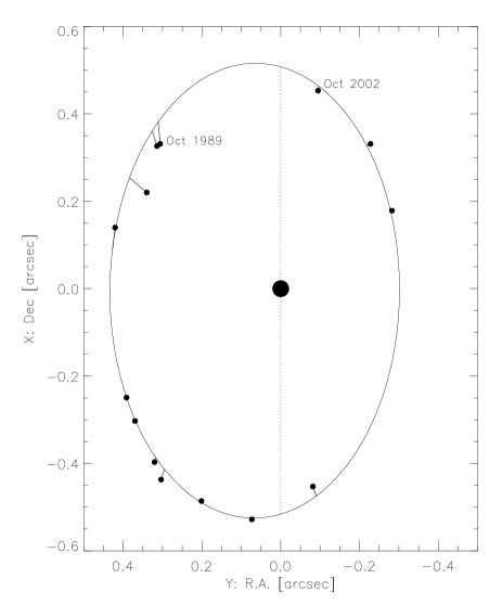
Figure 2: Upper panel: Our visual orbit for Gliese 22 AC, together with the residuals of the individual data points. The line of nodes is also indicated. The motion of the companion is anticlockwise. Lower panel: Comparison of our data points with all four orbits from Table 4: Our orbit (thick solid line) and the astrometric orbits from Hershey (Her73 (1973), dot-dot-dashed), Heintz (Hei93 (1993), dashed) and Söderhjelm (Sod99 (1999), dotted).

To calculate the visual orbit indicated in Fig. 2, we used the method proposed by Docobo (Doc85 (1985)). A weight from 4 to 10 was assigned to the individual measurements (see Table 1) to take into account seeing conditions and the quality of different instruments. The resulting orbital elements and their uncertainties are presented in Table 4 together with the results of the three previous astrometric orbital solutions. Ephemerides for $\theta$ and $\rho$ until epoch 2015.0 are given in Table 5. The residuals of our data points with respect to our visual orbit and the most recent astrometric orbit by Söderhjelm Sod99 (1999) (Table 6) indicate that our visual orbit represents a significant improvement. This is also evident from Fig. 2 (right panel) where our data points are plotted together with all four orbits. The precision of the orbital elements is rather high, and we expect only minor changes to this orbit. Thus, grade 2 (good orbit) can be assigned to it according to the grading scheme described in the Sixth Catalog of Orbits of Visual Binary Stars (Hartkopf & Mason Har03 (2003)).
The system mass derived from $a$ and $P$, using the Hipparcos parallax (98.74 $\pm$ 3.37 milli-arcsec) is equal to $0.592\pm 0.065M_{\sun}$. This represents a rather high relative accuracy as the direct dynamical mass sum determination concerned. While a good quality orbit (in particular, $a$ and $P$ are determined with an accuracy of almost 1%) is obtained, the accuracy of mass determination is still 11%. The latter is a good accuracy itself since the usual values for post-Hipparcos epoch are in the order of $20-25$% (see Martin et al. Mar98 (1998), Söderhjelm Sod99 (1999)) but it is worth noting that it could be even better.
The principal reason in this (and many other) cases is the low accuracy of the Hipparcos parallax (more than 3%) whose contribution to the mass error is 88% while semimajor axis and period contribution are almost insignificant (5% and 7% respectively). Gliese 22 AC is thus a good example of the overall mass accuracy deterioration due basically to the low relative accuracy of the parallax. Therefore, one must state that the sensibly higher accuracy next generation post-Hipparcos parallaxes are needed to drastically improve the relative accuracy of direct mass determination. Should semimajor axis, period and parallax be each determined with 1% accuracy, a mass determination accuracy of 5% can be achieved which is especially important for the lower end of luminosities in the HR diagram.

4 Discussion

We can now compare our dynamical mass with predictions from the present mass-luminosity relations on the lower main sequence as well as from theoretical evolutionary models for low-mass objcts. The absolute (system) K band magnitude for Gliese 22 AC is 6.26 $\pm$ 0.12 mag (McCarthy et al. Mcc91 (1991)) The mean flux ratio from all measurements in Table 1 is $F_{C}/F_{A}=0.156\pm 0.005$. This results in absolute magnitudes for the components:

$$K_{A} = 6.42\pm 0.12$$

$$K_{C} = 8.43\pm 0.13$$ (1)

The K band mass-luminosity relation given by Henry & McCarthy (Hen93 (1993), their Eq. 2) translates this into component masses:

$$M_{A}=0.378^{+0.028}_{-0.025}M_{\sun}$$

$$M_{C}=0.136^{+0.007}_{-0.007}M_{\sun}$$ (2)

The sum of these masses is $0.514\pm 0.029\,M_{\sun}$. The dynamical system mass of $0.592\pm 0.065\,M_{\sun}$ is in line with this result only within its $2\sigma$ error. McCarthy et al. (Mcc91 (1991)) did a similar calculation and found that the mass sum derived from the infrared magnitude-mass relations of Henry & McCarthy (Hen90 (1990)) and the dynamical mass were remarkably consistent. For the latter they used however the orbit calculation by Hershey (Her73 (1973)) which is worse than our visual orbit (see Fig. 2) and results in a probably too low system mass of $0.485\pm 0.071\,M_{\odot}$. Our result indicates that the the K band mass-luminosity relations by Henry & McCarthy probably underestimate stellar masses for M dwarfs. A similar result can be obtained for the optical mass-luminosity relation given by Henry et al. (Hen99 (1999)). Using resolved photometry taken with the HST Fine Guidance Sensors and updated parallax information (van Altena et al. Alt95 (1995)), these authors derive a system mass of $0.489\pm 0.041\,M_{\odot}$. This is again distinctly lower than our dynamical value.
The components’ K band magnitudes from Eq. 4 can also be used to derive masses from the theoretical evolutionary models for low-mass stars and substellar objects presented by Baraffe et al. (Bar98 (1998), Bar02 (2002)). For this purpose one has to assume an age for Gliese 22. Since this system shows no signs of chromospheric activity (H$\alpha$ is in absorption, see Herbst & Miller Her89 (1989)), we adopt a lower age limit of $10^{8}\,\mathrm{yr}$. As can be seen from Table 7, the system mass derived from the theoretical models is $\leq 0.54\,M_{\sun}$ for all ages above this value. This is again less than the dynamical system mass of $0.592\,M_{\sun}$, but comparable to this empirical result within the uncertainties. The restriction of this discussion to ages $\geq 10^{8}\,\mathrm{yr}$ causes no bias since lower ages would yield much lower (and thus unrealistic) mass estimates.
Gliese 22 AC is a variable star that shows flare events with amplitudes of 0.6 mag at optical wavelenghts (Pettersen Pet75 (1975)). One may ask how this property influences the previous discussion. Even in the unlikely case that the components’ magnitudes from Table 4 were affected by flares, our conclusions would not be altered. Temporary higher luminosities would lead to higher mass estimates, and thus the masses inferred from the mass-luminosity relation and theoretical evolutionary models would be even lower than our values if derived from observations in the quiescent state of a flare star.

Table 7: Masses for Gliese 22 A and C derived from their K magnitudes (Eq. 4) using the theoretical evolutionary models from Baraffe et al. (Bar98 (1998), Bar02 (2002)).

Age [yr]	$M_{A}[M_{\sun}]$	$M_{C}[M_{\sun}]$	$M_{Sys}[M_{\sun}]$
$10^{8}$	0.36	0.095	0.455
$10^{8.5}$	0.40	0.14	0.54
$10^{9}$	0.39	0.14	0.53
$10^{10}$	0.39	0.14	0.53

The lower mass component Gl 22 C is apparently a very low-mass star with a mass close to the hydrogen burning mass limit at $M\approx 0.075\,M_{\odot}$. Therefore, it would be very interesting to derive its individual dynamical mass from an absolute orbit and compare it to the predictions of theoretical models. It will probably indeed be possible to disentangle the relative orbit for Gliese 22 AC into two absolute orbits for both components using the distant companion Gliese 22 B as astrometric reference. However, to obtain most reliable absolute orbits, a complete coverage of an orbital revolution of the AC pair is strongly desirable, and this is thus beyond the scope of this paper.

5 Summary

With the first calculation of a purely visual orbit from interferometric data we have largely improved on the accuracy of the orbital elements for the low-mass binary Gliese 22 AC and derived a dynamical system mass of $0.592\pm 0.065\,M_{\sun}$. The uncertainty of 11% is mostly due to the error of the Hipparcos parallax, while future ($\rho$, $\theta$) measurements will probably result in only minor changes of the orbital parameters. Based on the K band magnitudes of the components we have estimated their masses also from the mass-luminosity relation given by Henry & McCarthy (Hen93 (1993)) and from the theoretical evolutionary models for low-mass objects by Baraffe et al. (Bar98 (1998), Bar02 (2002)). In both cases the obtained mass sum is lower than the dynamical system mass. The component Gliese 22 C is apparently a very low-mass star with a mass around $0.1\,M_{\sun}$ and is thus located at the very end of the lower main sequence.

- (1) Alden, H.L. 1947, AJ, 52, 138
- (2) Baraffe, I., Chabrier, G., Allard, F., Hauschildt, P.H. 1998 A&A, 337, 403
- (3) Baraffe, I., Chabrier, G., Allard, F., Hauschildt, P.H. 2002 A&A, 382, 563
- (4) Docobo, J.A. 1985, Celestial Mechanics, 36, 143
- (5) Docobo, J.A., Tamazian, V.S., Woitas, J., & Leinert, Ch. 2002, IAU Comm. 26 Inf. Circ. 147
- (6) Espin, Rev., T.E., Milburn, E. 1926, MNRAS, 86, 131
- (7) Hartkopf, W.I., Mason, B.D. 2003, The Sixth Catalog of Orbits of Visual Binary Stars, http://ad.usno.navy.mil/wds/orb6.html
- (8) Heintz, W.D. 1993, PASP, 105, 44
- (9) Herbst, W., Miller, J.R. 1989, AJ, 97, 891
- (10) Henry, T.J. 1998, ASP Conference Series, 134, 28
- (11) Henry, T.J., McCarthy, D.W. 1990, ApJ, 350, 334
- (12) Henry, T.J., McCarthy, D.W. 1993, AJ, 106, 773
- (13) Henry, T.J., Franz, O.G., Wasserman, L.H., et al. 1999, ApJ, 512, 864
- (14) Hershey, J.L. 1973, AJ, 78, 935
- (15) Knox, K.T., & Thompson, B.J. 1974, ApJ, 193, 45
- (16) Köhler, R., Kunkel, M., Leinert, Ch., Zinnecker, H. 2000, A&A, 356, 541
- (17) Lampens, P., Strigachev, A. 2001, A&A, 368, 572
- (18) Leinert, Ch., & Haas, M. 1989, A&A, 221, 110
- (19) Leinert, Ch., Jahreiß, H., Woitas, J., et al. 2001, A&A, 367, 183
- (20) Lohmann, A.W., Weigelt, G., Wirnitzer, B. 1983, App. Opt., 22, 4028
- (21) Martin, C., Mignard, F., Hartkopf, McAllister, H.A. 1998, A&AS, 133, 149
- (22) McCarthy, Jr., D.W., Henry, T.J., McLeod, B., Christou, J.C. 1991, AJ, 101, 214
- (23) McCaughrean, M.J., Stauffer, J.R. 1994, AJ, 108, 1382
- (24) Pettersen, B.R. 1975, A&A, 41, 113
- (25) Scardia, M. 1983, A&AS, 53, 177
- (26) Söderhjelm, S. 1999, A&A, 341, 121
- (27) van Altena, W.F., Lee, J.T., & Hoffleit, E.D. 1995, The General Catalogue of Trigonometric Stellar Parallaxes, Fourth Edition, Yale University Observatory
- (28) Woitas, J., Leinert, Ch., Jahreiß, H., et al. 2000, A&A, 353, 253