The primary cosmic ray composition between $10^{15}$ and $10^{16}$ eV from Extensive Air Showers electromagnetic and TeV muon data

Abstract

The cosmic ray primary composition in the energy range between $10^{15}$ and $10^{16}$ eV, i.e., around the “knee” of the primary spectrum, has been studied through the combined measurements of the EAS-TOP air shower array (2005 m a.s.l., 10⁵ m² collecting area) and the MACRO underground detector (963 m a.s.l., 3100 m w.e. of minimum rock overburden, 920 m² effective area) at the National Gran Sasso Laboratories. The used observables are the air shower size ($N_{e}$) measured by EAS-TOP and the muon number ($N_{\mu}$) recorded by MACRO. The two detectors are separated on average by 1200 m of rock, and located at a respective zenith angle of about 30^∘. The energy threshold at the surface for muons reaching the MACRO depth is approximately 1.3 TeV. Such muons are produced in the early stages of the shower development and in a kinematic region quite different from the one relevant for the usual $N_{\mu}-N_{e}$ studies. The measurement leads to a primary composition becoming heavier at the knee of the primary spectrum, the knee itself resulting from the steepening of the spectrum of a primary light component (p, He). The result confirms the ones reported from the observation of the low energy muons at the surface (typically in the GeV energy range), showing that the conclusions do not depend on the production region kinematics. Thus, the hadronic interaction model used (CORSIKA/QGSJET) provides consistent composition results from data related to secondaries produced in a rapidity region exceeding the central one. Such an evolution of the composition in the knee region supports the “standard” galactic acceleration/propagation models that imply rigidity dependent breaks of the different components, and therefore breaks occurring at lower energies in the spectra of the light nuclei.

1 Introduction

The study of the primary cosmic ray composition and of its evolution with primary energy is the main tool in understanding the cosmic ray acceleration processes. In particular the energy range between $10^{15}$ and $10^{16}$ eV is characterized by breaks in the size spectra of the different Extensive Air Shower (EAS) components: electromagnetic (e.m.) [1], muon [2], Cherenkov light [3], and hadrons [4], which are therefore interpreted as a break in the primary energy spectrum. It is now recognized that the interpretation of such a feature could provide a significant signature in understanding the galactic cosmic radiation [5], [6], [7], [8], [9].

Independent measurements based on the observation of the e.m. and GeV muon components [10], [11] lead to a composition becoming heavier in this energy region. The situation is more complex when other components are considered, thus showing that further information is needed from independent observables (see, e.g., [12] and references therein). This is also useful to cross check the information, reduce the dependence on the hadron interaction model and particle propagation codes used, and to have better control of fluctuations in shower development, and therefore of event selection.

At the National Gran Sasso Laboratories, we have developed a program of systematic study of the surface shower size measurements from EAS-TOP and the high energy muons ($E_{\mu}^{th}=1.3$ TeV) measured deep underground (MACRO). Such muons originate from the decays of mesons produced in the first interactions of the incident primary in the atmosphere, and thus are from a quite different rapidity region than the GeV muons usually used for such analyses ($x_{F}>0.1$ or $0.2$, the rapidity region being $y-y_{beam}\approx-(4.5-5.0)$ at $\sqrt{s}\approx 1000$ TeV). The experiment provides therefore new data related to the first stages of the shower development, from secondaries produced beyond the central rapidity region.

EAS-TOP and MACRO operated in coincidence in their respective final configurations for a live time of $\Delta T=$ 23,043 hours between November 25, 1992 and May 8, 2000, corresponding to an exposure ${\Gamma\cdot\Delta T}\approx 4\times 10^{9}$ m² s sr. We present here an analysis of the full data set. Further details and partial results of the present work can be found in [13], [14] and [15].

2 The detectors

The EAS-TOP array was located at Campo Imperatore (2005 m a.s.l., at about $30^{\circ}$ from the vertical at the underground Gran Sasso Laboratories, corresponding to an atmospheric depth of 930 g cm^-2). Its e.m. detector (in which we are mainly interested in the present analysis) was built of 35 scintillator modules each 10 m² in area, resulting in a collecting area A $\approx$ 10⁵ m². The array was fully efficient for $N_{e}>10^{5}$. In the following analysis, we will use events with at least 7 neighboring detectors fired and a maximum particle density recorded by an inner module (“internal events”). The EAS-TOP reconstruction capabilities of the EAS parameters for such events are: ${{\Delta N_{e}}\over N_{e}}\approx 10\%$ above $N_{e}\approx 10^{5}$ for the shower size, and $\Delta\theta\approx 0.9^{\circ}$ for the arrival direction. The array and the reconstruction procedures are fully described in [16].

MACRO, in the underground Gran Sasso Laboratories at 963 m a.s.l., with 3100 m w.e. of minimum rock overburden, was a large area multi-purpose apparatus designed to detect penetrating cosmic radiation. A detailed description of the apparatus can be found in [17]. In this work we consider only muon tracks which have at least 4 aligned hits in both views of the horizontal streamer tube planes out of the 10 layers composing the lower half of the detector, which had dimensions $76.6\times 12\times 4.8$ m³. The MACRO standard reconstruction procedure [18] has been used, which provides an accuracy due to instrumental uncertainties and muon scattering in the rock of $0.95^{\circ}$ for the muon arrival direction. The muon number is measured with an accuracy $\Delta N_{\mu}<1$ for multiplicities up to $N_{\mu}\approx 10$, and $\Delta N_{\mu}\approx 1$ for $N_{\mu}>10$; high multiplicity events have been scanned by eye to avoid possible misinterpretations.

The two experiments are separated by a rock thickness ranging from 1100 to 1300 m, depending on the angle. The energy threshold at the surface for muons reaching the MACRO depth ranges from $E_{\mu}^{th}=1.3$ TeV to $E_{\mu}^{th}=1.8$ TeV within the effective area of EAS-TOP.
The two experiments operated with independent triggering conditions, set to 1) four nearby detectors fired for EAS-TOP (corresponding to a primary energy threshold of about 100 TeV), and 2) a single muon in MACRO. Event coincidence is established off-line, using the absolute time given by a GPS system with an accuracy better than 1 $\mu s$. The number of coincident events amounts to 28,160, of which 3,752 are EAS-TOP “internal events” (as defined above) and have shower size $N_{e}>2\times 10^{5}$; among them 409 have $N_{e}>10^{5.92}$, i.e., are above the knee observed at the corresponding zenith angle [19]. We present here the analysis of such events, by using full simulations 1) of the detectors (based on GEANT [20]), 2) of the cascades in the atmosphere performed within the same framework as for the surface data (CORSIKA/QGSJET [21]), and 3) of the MUSIC code [22] for muon transport in the rock. Independent analyses from the two experiments separately are reported in [23], [19] and [11].

3 Analysis and results

3.1 The data

The experimental quantities considered are the muon multiplicity distributions (for $N_{\mu}\geq 1$ as required by the coincidence trigger condition) in several intervals of shower sizes. We have chosen six intervals of shower sizes covering the region of the knee:
5.20 $<Log_{10}(N_{e})\leq$ 5.31 (1432 events), 5.31 $<Log_{10}(N_{e})\leq$ 5.61 (2352 events), 5.61 $<Log_{10}(N_{e})\leq$ 5.92 (881 events), 5.92 $<Log_{10}(N_{e})\leq$ 6.15 (252 events), 6.15 $<Log_{10}(N_{e})\leq$ 6.35 (106 events) and 6.35 $<Log_{10}(N_{e})\leq$ 6.70 (42 events). The experimental relative frequencies of the multiplicity distributions are shown in Fig.1. For further analysis, the data have been grouped in variable multiplicity bin sizes reported with their contents in Tables 1–6.

	Exp. data.		MC Light		MC Heavy		Fit Light+Heavy
Nμ	fev	$\sigma_{f_{ev}}~{}(\%)$	fev	$\sigma_{f_{ev}}$	fev	$\sigma_{f_{ev}}~{}(\%)$	fev	$\sigma_{f_{ev}}~{}(\%)$
1–2	0.7353	3.1	0.7878	2.3	0.5656	3.2	0.7381	10.7
3–4	0.1927	6.0	0.1706	5.0	0.2436	4.9	0.1866	13.6
5–6	0.0475	12.2	0.0344	11.0	0.1206	7.0	0.0534	20.6
7–8	0.0189	19.0	0.0055	27.3	0.0509	10.8	0.0155	29.0
9–10	0.0028	50.0	0.0013	53.8	0.0135	20.7	0.0040	30.0
11–12	0.0007	100.0	0.0004	100.0	0.0053	34.0	0.0015	44.1
13–14	0.0014	71.4	0.0	0.0	0.0006	100.0	0.0001	100.0

Table 1: Relative frequency multiplicity distribution for size window: $5.20<Log_{10}(N_{e})<5.31$ (1432 events). The simulated distributions are also reported for the Light, Heavy components Monte Carlo (MC), and the resulting fit (see text). The number of digits is chosen in order to show the one event level.

	Exp. data.		MC Light		MC Heavy		Fit Light+Heavy
Nμ	fev	$\sigma_{f_{ev}}~{}(\%)$	fev	$\sigma_{f_{ev}}$	fev	$\sigma_{f_{ev}}~{}(\%)$	fev	$\sigma_{f_{ev}}~{}(\%)$
1–2	0.6743	2.5	0.7292	1.9	0.5147	2.7	0.6764	8.2
3–4	0.1973	4.7	0.1907	3.7	0.2010	4.2	0.1932	8.0
5–6	0.0782	7.5	0.0591	6.6	0.1472	5.0	0.0806	13.2
7–8	0.0344	11.0	0.0163	12.9	0.0836	6.6	0.0328	17.6
9–10	0.0098	20.4	0.0023	34.7	0.0374	9.9	0.0109	23.9
11–12	0.0030	36.7	0.0016	37.5	0.0109	18.3	0.0038	21.1
13–14	0.0017	52.9	0.0008	62.5	0.0036	30.6	0.0015	20.0
15–16	0.0009	66.7	0.0	0.0	0.0007	71.4	0.0002	50.0
17–18	0.0004	100.0	0.0	0.0	0.0	0.0	0.0	0.0
19–20	0.0	0.0	0.0	0.0	0.0007	71.4	0.0	0.0

Table 2: As Table 1 for size window: $5.31<Log_{10}(N_{e})<5.61$ (2352 events).

	Exp. data.		MC Light		MC Heavy		Fit Light+Heavy
Nμ	fev	$\sigma_{f_{ev}}~{}(\%)$	fev	$\sigma_{f_{ev}}$	fev	$\sigma_{f_{ev}}~{}(\%)$	fev	$\sigma_{f_{ev}}~{}(\%)$
1–2	0.6118	4.3	0.6131	2.9	0.4412	4.1	0.5741	12.6
3–4	0.1839	7.9	0.2341	4.7	0.1689	6.7	0.2193	12.7
5–6	0.0885	11.3	0.0972	7.4	0.1214	7.9	0.1019	15.1
7–8	0.0568	14.1	0.0370	11.9	0.0988	8.7	0.0498	21.5
9–10	0.0272	20.6	0.0127	20.5	0.0799	9.8	0.0268	31.0
11–12	0.0170	25,9	0.0053	32.0	0.0483	12.4	0.0143	35.0
13–14	0.0068	41.2	0.0	0.0	0.0219	18.7	0.0046	50.0
15–16	0.0045	60.0	0.0005	100.0	0.0106	26.4	0.0026	42.3
17–18	0.0011	100.0	0.0	0.0	0.0030	50.0	0.0006	50.0
19–20	0.0011	100.0	0.0	0.0	0.0030	50.0	0.0006	50.0
21–28	0.0011	100.0	0.0	0.0	0.0030	50.0	0.0006	50.0

Table 3: As Table 1 for size window: $5.61<Log_{10}(N_{e})<5.92$ (881 events).

	Exp. data.		MC Light		MC Heavy		Fit Light+Heavy
Nμ	fev	$\sigma_{f_{ev}}~{}(\%)$	fev	$\sigma_{f_{ev}}$	fev	$\sigma_{f_{ev}}~{}(\%)$	fev	$\sigma_{f_{ev}}~{}(\%)$
1–2	0.5318	8.6	0.4992	5.7	0.4353	7.0	0.4698	26.9
3–4	0.1786	14.9	0.2373	8.3	0.1315	12.8	0.1936	26.3
5–6	0.0833	21.8	0.1309	11.2	0.1013	14.6	0.1182	26.6
7–8	0.0714	23.5	0.0687	15.4	0.0927	15.2	0.0776	28.7
9–10	0.0318	35.2	0.0426	19.5	0.0754	17.0	0.0552	30.6
11–12	0.0476	29.0	0.0147	33.3	0.0582	19.2	0.0317	37.5
13–14	0.0198	44.9	0.0033	69.7	0.0409	23.0	0.0181	45.3
15–16	0.0159	49.7	0.0016	100.0	0.0259	29.0	0.0112	45.5
17–18	0.0119	58.0	0.0016	100.0	0.0172	35.5	0.0078	43.6
19–24	0.0040	100.0	0.0000	0.0	0.0151	37.7	0.0060	50.0
25–30	0.0040	100.0	0.0000	0.0	0.0065	56.9	0.0026	50.0

Table 4: As Table 1 for size window: $5.92<Log_{10}(N_{e})<6.15$ (252 events).

	Exp. data.		MC Light		MC Heavy		Fit Light+Heavy
Nμ	fev	$\sigma_{f_{ev}}~{}(\%)$	fev	$\sigma_{f_{ev}}$	fev	$\sigma_{f_{ev}}~{}(\%)$	fev	$\sigma_{f_{ev}}~{}(\%)$
1–2	0.4245	14.9	0.4271	8.9	0.3585	11.5	0.3818	39.5
3–4	0.1698	23.6	0.1966	13.1	0.1557	17.4	0.1692	39.9
5–6	0.0849	33.3	0.1492	15.1	0.0566	28.8	0.0857	48.2
7–8	0.0849	33.3	0.1085	17.7	0.1085	20.8	0.1091	38.5
9–10	0.0472	44.7	0.0475	26.7	0.0708	25.8	0.0639	37.4
11–12	0.0377	50.1	0.0475	26.7	0.0566	28.8	0.0541	37.9
13–14	0.0849	33.3	0.0102	57.8	0.0708	25.8	0.0523	40.0
15–16	0.0189	70.4	0.0068	70.6	0.0377	35.3	0.0283	39.6
17–18	0.0189	70.4	0.0000	0.0	0.0236	44.5	0.0164	42.1
19–20	0.0094	100.0	0.0000	0.0	0.0094	71.3	0.0066	42.4
21–22	0.0094	100.0	0.0034	100.0	0.0189	49.7	0.0142	39.4
23–26	0.0094	100.0	0.0034	100.0	0.0189	49.7	0.0142	39.4
27–30	0.0	0.0	0.0	0.0	0.0141	58.2	0.0098	41.8

Table 5: As Table 1 for size window: $6.15<Log_{10}(N_{e})<6.35$ (106 events).

	Exp. data.		MC Light		MC Heavy		Fit Light+Heavy
Nμ	fev	$\sigma_{f_{ev}}~{}(\%)$	fev	$\sigma_{f_{ev}}$	fev	$\sigma_{f_{ev}}~{}(\%)$	fev	$\sigma_{f_{ev}}~{}(\%)$
1–2	0.5238	21.3	0.3712	10.9	0.3765	12.5	0.3752	57.5
3–4	0.1429	40.8	0.2096	14.5	0.1294	21.3	0.1486	64.7
5–6	0.0952	50.0	0.1441	17.4	0.0882	25.9	0.1016	64.9
7–8	0.0476	70.8	0.0699	25.0	0.0471	35.2	0.0526	62.9
9–10	0.0238	100.0	0.0611	26.7	0.0529	33.3	0.0549	59.4
11–14	0.0476	70.8	0.1310	18.2	0.1353	20.8	0.1343	57.4
15–18	0.0476	70.8	0.0087	71.3	0.0471	35.2	0.0379	56.2
19–22	0.0238	100.0	0.0044	100.0	0.0412	37.9	0.0324	57.4
23–26	0.0238	100.0	0.0000	0.0	0.0471	35.2	0.0358	59.5
27–30	0.0238	100.0	0.0000	0.0	0.0353	40.8	0.0269	56.9

Table 6: As Table 1 for size window: $6.35<Log_{10}(N_{e})<6.70$ (42 events).

Figure 1: Distributions of the relative frequencies of the detected underground muon multiplicities in the 6 selected size windows. See Tables 1–6. Notice the expected increasing relative frequency of high multiplicity events as a function of shower size.

3.2 The simulation

We have simulated atmospheric showers in an energy range which includes the e.m. size values considered here (between 100 and 100,000 TeV/particle) and in an angular range exceeding the aperture of the coincidence experiment. Shower simulations have been performed with the QGSJET [24] hadronic interaction model implemented in CORSIKA v5.62 [21] . Primary particles have been sampled in a solid angle region of the order of the area encompassing the surface array as seen from the underground detector. The solid angle corresponding to the selected angular window is $\Omega=0.0511$  sr. All muons with energy $E_{\mu}\geq$ 1 TeV reaching the surface have been propagated through the rock down to the MACRO depth by means of the muon transport code MUSIC [22]; the accuracy of this transport code has been verified by comparing its results to those achieved with other Monte-Carlo simulations. Generated events having no muons surviving underground have been discarded, while those having at least one surviving muon have been folded with the underground detector simulation according to the following method, whose theoretical principles are discussed in [29]. We have considered an array of 39 (13 $\times$ 3) identical MACRO detectors adjacent to one another, covering an area of 230.7 $\times$ 158.2 m². The shower axis is sampled over the horizontal area of the central MACRO, and all hit detectors are considered. For each hit detector, the full GMACRO (GEANT based) simulation of MACRO is invoked and is considered as a different event. For each of these events, when considered at the position of the “real” MACRO, the position of the shower core at the surface is recalculated, the particle densities on EAS-TOP counters are calculated and the trigger simulation is then invoked. Particle densities are obtained from the lateral distribution of the e.m. component of the shower as produced by CORSIKA (with the analytical “Nishimura-Kamata-Greisen” option), taking into account the fluctuations of the number of particles hitting the detector modules and the full detectors’ fluctuations [16]. If the trigger threshold is reached, the reconstructions of both EAS-TOP and MACRO are activated, thus producing results in the same format as the real data. The resulting events, after combining the simulated reconstructions of surface and underground detectors, are eventually stored as simulated coincidence events. Five samples with different nuclear masses have been generated: proton, Helium, Nitrogen (CNO), Magnesium and Iron, all with the same spectral index $\gamma=2.62$. Shower size bins have been chosen to be small enough so that no significant change in the shape of the muon multiplicity distributions in each bin is observed for different, extreme spectral indexes. A number of events exceeding the experimental statistics have been simulated in each size bin.

3.3 The results

The analysis is performed through independent fits of the experimental muon multiplicity distributions in the selected intervals of shower size. The simulated multiplicity distributions have been used as theoretical expectations for the individual components, and the relative weights are the fit parameters.

The possibility that the experimental data could be reproduced with a single mass component can be easily excluded for the extreme (p or Fe) components, but also for medium mass primaries (e.g., A = 14): the obtained values of ${\chi}^{2}$ are not satisfactory (too large, the point will be addressed at the end of the section). On the other hand, with a number of components larger than two we cannot achieve better solutions, since in all cases the minimization algorithm tends to force to zero the contribution of an intermediate component. This is mainly due to our limited statistics. For this reason we performed our analysis by considering only two components in the primary beam. We have tested two cases: a combination of p and Fe components, and a combination of two admixtures: a “Light” ($L$) and “Heavy” ($H$) one, built with equal fractions of p plus He and Mg plus Fe, respectively. Preliminary results from the p+Fe analysis have been presented in [15, 28]. Here we describe the final analysis in terms of the $L$+$H$ admixtures.

The fit has been performed in the six quoted size windows by minimizing the following expression for each multiplicity distribution:

$$\xi^{2}=\sum_{i}{\frac{(N^{exp}_{i}-p_{L}N^{L}_{i}-p_{H}N^{H}_{i})^{2}}{\sigma_{i,exp}^{2}+(p_{L}\sigma_{i,L})^{2}+(p_{H}\sigma_{i,H})^{2}}}$$ (1)

where $N^{exp}_{i}$ is the number of events observed in the $i^{th}$ bin of multiplicity (with statistical uncertainty $\sigma_{i,exp}$), $N^{L}_{i}$ and $N^{H}_{i}$ are the numbers of simulated events in the same $i^{th}$ multiplicity bin from the $L$ and $H$ components, respectively, $p_{L}$ and $p_{H}$ are the parameters (to be fitted) defining the fraction of each mass component contributing to the same multiplicity bin, and $\sigma_{i,L}$ and $\sigma_{i,H}$ are the statistical errors of the simulation. Such an expression is close to that of a $\chi^{2}$, although, in principle, it follows a different statistics, and in the following we shall refer to it as if it were a genuine $\chi^{2}$. The values of the parameters $p_{L}$ and $p_{H}$ obtained from the minimizations are given in Table 7. The progressive decrease of the “Light” component in favor of the “Heavy” one is visible and significant at the level of 2 standard deviations: the average $p_{L}$ value is 0.70 $\pm$ 0.04 below the observed knee in size (Log₁₀($N_{e}$) = 5.92), and 0.28 $\pm$ 0.17 above. By normalizing $p_{L}$ and $p_{H}$ to the observed number of coincident events in each size bin (see Tables 1–6) we obtain the contribution to the measured size spectrum of each component.

Log10($N_{e}$) window	pL	pH	$\chi^{2}$/Nd.o.f.
5.20–5.31	0.74 $\pm$ 0.07	0.26 $\pm$ 0.11	5.5/5
5.31–5.61	0.70 $\pm$ 0.05	0.30 $\pm$ 0.09	2.7/7
5.61–5.92	0.66 $\pm$ 0.09	0.34 $\pm$ 0.14	11.4/9
5.92–6.15	0.50 $\pm$ 0.17	0.50 $\pm$ 0.24	12.2/9
6.15–6.35	0.30 $\pm$ 0.20	0.70 $\pm$ 0.32	4.7/10
6.35–6.70	0.24 $\pm$ 0.32	0.76 $\pm$ 0.45	8.4/8

Table 7: The fitted normalizations for the two components (L, H) as a function of size (notice that the two parameters are correlated, so that errors are not independent from one another).

In Fig. 2 the multiplicity distributions are shown for the four most relevant size windows, together with the expected $L$ and $H$ components, and their best fit combination.

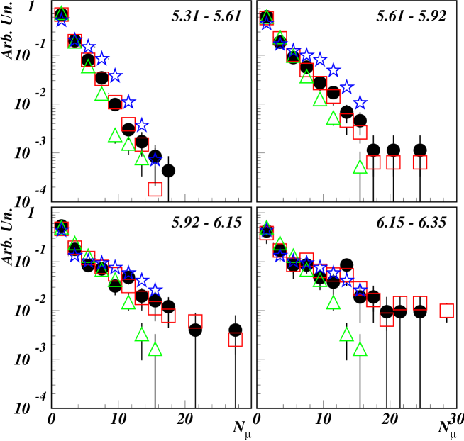
Figure 2: Distributions of the relative frequencies of the detected underground muon multiplicities (black points) together with the predictions for $L$ (open triangles) and $H$ (open stars) admixtures in the QGSJET interaction model, and the ($L$+$H$) fit (open squares).

Regarding the shapes of the multiplicity distributions, it is interesting to remark that they cannot be described by simple single laws, and show some structure; this is evident in the data and in the simulated Heavy components, however less so in the simulated Light ones. The origin of such structure is entirely geometric and due to the interplay between the typical size of muon bundles with the two length scales of the MACRO detector. Small bundle sizes can be entirely contained in the detector while, when the size increases, this becomes impossible along the width of the detector. Bundles of even larger size exceed also the length of MACRO. This fact is well taken into account by the simulation, and in fact the fit reproduces correctly this change of structure, which is typical of large bundles (i.e., high energies and large masses). The effect is evident when comparing with a single component fit, say the CNO group that has an intermediate average atomic number. The results of the fit are presented in Fig. 3. CNO primaries alone provide good fits in the higher size bins (due to the limited statistics), but below and just above the knee at $Log_{10}(N_{e})=5.92$, the large $\chi^{2}$ values indicate the failure to reproduce the shape of the multiplicity distribution (see Table 8).

Log10($N_{e}$) window	$\chi^{2}$/Nd.o.f.
5.20–5.31	17.3/6
5.31–5.61	49.9/8
5.61–5.92	45.6/10
5.92–6.15	16.8/10
6.15–6.35	4.7/11
6.35–6.70	8.7/9

Table 8: The $\chi^{2}$ values resulting from the fits to the CNO (A=14) component alone, as a function of shower size.

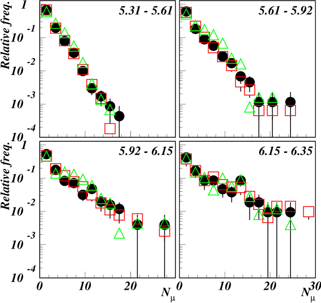
Figure 3: Distributions of the relative frequencies of the detected underground muon multiplicities (black symbols) together with the results of the fits for the QGSJET interaction model ($L$+$H$) (open squares), compared with a fit with the CNO component only (open triangles).

3.4 Interpretation of the data

For a given size window, the contribution of each primary mass group derives from a different energy region: the higher the mass number, the higher the corresponding energy. The size-energy mapping far from shower maximum is model dependent, and in our analysis is based on CORSIKA/QGSJET. From the full simulation chain we also calculate the probabilities $\epsilon_{\alpha}(E,\Delta_{i}N_{e})$ for a primary belonging to mass group $\alpha$ ($\alpha~{}=~{}L,~{}H$) and of energy $E$ to give a coincident event in the $i^{th}$ size window $\Delta_{i}N_{e}$. To evaluate the average mass composition we use a logarithmic energy binning (3 bins per energy decade), starting from 100 TeV/nucleus. From the simulation we obtain the number of events ($n^{\alpha}_{j}(\Delta_{i}N_{e})$) that a primary of mass group $\alpha$ will produce in the $j^{th}$ energy bin, when the detected size is in the windows $\Delta_{i}N_{e}$. Therefore the total number of events that the primary mass group $\alpha$ produces in the size window $\Delta_{i}N_{e}$ is the sum of $n^{\alpha}_{j}(\Delta_{i}N_{e})$ over the energy bins.

We require that the number of experimentally observed events in the size window $\Delta_{i}N_{e}$ be equal to:

$$N^{exp}(\Delta_{i}N_{e})=p^{L}(\Delta_{i}N_{e})\sum_{j}{n^{L}_{j}(\Delta_{i}N_{e})}+p^{H}(\Delta_{i}N_{e})\sum_{j}{n^{H}_{j}(\Delta_{i}N_{e})}$$ (2)

where $p^{L}$ and $p^{H}$ are the fit coefficients for the given size window $\Delta_{i}N_{e}$. These are normalized, so that $p^{L}=1-p^{H}$ in each size window. This leaves an overall renormalization factor $K$ free in order to satisfy eq.2, so we obtain the renormalized quantities $n^{*\alpha}_{j}~{}=~{}K~{}n^{\alpha}_{j}$. The corrected estimated number of primaries of mass group $\alpha$ for each size window belonging to energy bin $j$ can thus be obtained by applying the efficiencies $\epsilon_{\alpha}(E_{j},\Delta_{i}N_{e})$:

$$m^{\alpha}_{j}(\Delta_{i}N_{e})=p^{\alpha}(\Delta_{i}N_{e}){n^{*\alpha}_{j}(\Delta_{i}N_{e})/\epsilon_{\alpha}(E_{j},\Delta_{i}N_{e})}$$ (3)

Then, since the $j^{th}$ energy bin may receive contributions from different size windows, we have to sum over $i$ (the size window index):

$$M^{\alpha}_{j}=\sum_{i}m^{\alpha}_{j}(\Delta_{i}N_{e})=\sum_{i}{p^{\alpha}(\Delta_{i}N_{e}){n^{*\alpha}_{j}(\Delta_{i}N_{e})/\epsilon_{\alpha}(E_{j},\Delta_{i}N_{e})}}$$ (4)

$M^{L}_{j}$ and $M^{H}_{j}$ provide estimates of the energy spectra of the $L$ and $H$ mass groups, presented in Fig. 4. There we plot the spectra starting from $10^{3}$ TeV since with our selection of size, this is the energy at which the heaviest component has reached a significant triggering efficiency.

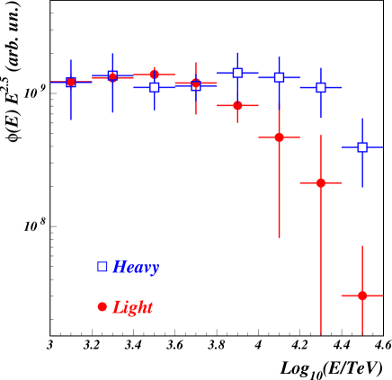
Figure 4: Energy spectra estimates for $L$ and $H$ admixtures.

A steepening by about $\Delta\gamma=0.7\pm 0.4$ of the light mass group spectrum just at the knee ($\sim$4$\times$10¹⁵ eV) is observed, assuming power law behaviors crossing at the knee position. Although these distributions cannot be used to obtain a direct representation of the actual cosmic ray spectrum, due to the two mass groups schematization and the choices of their components, the relative proportion of “Light” and “Heavy” admixtures turns out to be quite stable with respect to the mentioned parameters; within this approximation, the resulting all-particle spectrum would show a $\Delta\gamma=0.4\pm 0.1$.

We make use of the values of $M^{L}_{j}$ and $M^{H}_{j}$ so obtained to compute the mean value of the natural logarithm of the primary mass ($<\ln A>$) as a function of energy:

$$<\ln A(E_{j})>=\frac{\ln A^{L}~{}M^{L}_{j}+\ln A^{H}~{}M^{L}_{j}}{M^{L}_{j}+M^{H}_{j}}$$ (5)

with $lnA^{L}=0.5(lnA^{p}+lnA^{He})$, and $lnA^{H}=0.5(lnA^{Mg}+lnA^{Fe})$. The uncertainty on $<\ln A(E_{j})>$ has been obtained by propagating the uncertainties on the fit coefficients. The result is reported in Fig. 5 together with the results of KASCADE [10] and EAS-TOP alone [11], where these analyses has been performed using e.m. size and GeV muons detected at surface level. The good agreement shows that the results do not depend on the selected muon energy. The $<\ln A(E_{j})>$ obtained by MACRO alone [23], on the basis of the HEMAS Monte Carlo code [30], has a milder energy dependence and appears to be in contrast with those presented here above $Log_{10}(E)>4.2$. In our opinion this is due to a weakness of the HEMAS model, based on parameterizations of UA5 results [31]. The possible shortcomings of the HEMAS model were already discussed in [32, 33].

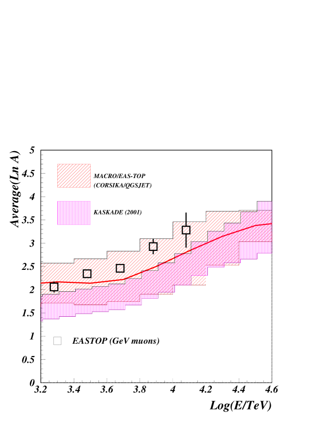
Figure 5: $<lnA>$ vs primary energy (continuous line). The hatched areas represent the 68% uncertainty range due to the statistical error. We also superimpose the results of KASCADE [10] and of EAS-TOP [11] (open squares).

The allowed region for $<lnA(E)>$ obtained from our analysis is also consistent with the theoretical expectations from refs. [9], [34], and [35].

4 Conclusions

The analysis N_e-N${}_{\mu}^{TeV}$ events collected by the MACRO/EAS-TOP Collaboration at the Gran Sasso Laboratories points to a primary composition becoming heavier around the knee of the primary spectrum (i.e., in the energy region $10^{15}-10^{16}$ eV). The result is in good agreement with the measurements of other experiments based on the observation of the e.m. and muon components at ground level. The muon energies detected in the present experiment are however about three orders of magnitude larger than in previous N_e-N_μ experiments, and therefore the parent pions are produced in a different kinematic region (at the edges of the fragmentation region, rather than in the central one) and in the first stages of the cascade development. A good overall consistency of the interaction model used (CORSIKA/QGSJET) in describing the yield of secondaries over a wide rapidity region is thus obtained. The present data explain therefore the observed knee in the cosmic ray primary spectrum as due to the steepening of the spectrum of a light component (p, He) at $E_{0}\approx 4\times 10^{15}$ eV, of $\Delta\gamma=0.7\pm 0.4$. Such an effect can be interpreted in the “standard” framework of the acceleration/propagation processes of galactic cosmic radiation that predict, as a general feature, rigidity dependent breaks for the different nuclei, and therefore appearing at lower energies for the lighter ones.

References

- [1] Kulikov G.V. and Khristiansen G.B., JEPT, 35, 635 (1958)
- [2] Navarra G. et al. (EAS-TOP Coll.), Nucl. Phys. B (Proc. Suppl.), 60, 105 (1998)
- [3] Gress O.A. et al. (Tunka Coll.), Proc. 25th ICRC (Durban, South Africa), 4, 129 (1997)
- [4] Hoerandel J.R. et al.(KASCADE Coll), Proc. 27th ICRC (Hamburg, Germany), 1, 137 (2001).
- [5] Peters B., Proc 6th ICRC (Moscow, USSR), 3, 157 (1959)
- [6] Zatsepin G.T. et al, Izv. Akad. Nauk USSR SP, 26, 685 (1962)
- [7] Hillas A.M., Proc 16th ICRC (Kyoto, Japan), 8, 7 (1979)
- [8] Bierman P.L., Proc 23rd ICRC (Calgary, Canada), Invited, Rapporteurs and Highlight Papers, 45 (1994)
- [9] Erlykin A.D. and Wolfendale A.W., J. Phys. G 23, 979 (1997)
- [10] Kampert K-H et al. (KASCADE Coll.), 27th ICRC (Hamburg, Germany), Invited, Rapporteurs and Highlight papers, 240 (2001); astro-ph/0212481, submitted to J. Phys. G.
- [11] Alessandro B. et al. (EAS-TOP Coll.), Proc. Vulcano Workshop 2002 (in press); Proc. 27th ICRC (Hamburg, Germany), 1, 124 (2001)
- [12] Sommers P., 27th ICRC (Hamburg, Germany), Invited, Rapporteurs and Highlights Papers, 170 (2001)
- [13] Bellotti R. et al. (EAS-TOP and MACRO Coll.), Phys. Rev D, 42, 1396 (1990)
- [14] Aglietta M. et al (EAS-TOP and MACRO Coll.), Phys. Lett. B, 337, 376 (1994)
- [15] Navarra G. et al. (EAS-TOP and MACRO Coll.), Proc. 27th ICRC (Hamburg, Germany), 1, 120 (2001)
- [16] Aglietta M. et al. (EAS-TOP Coll.), Nucl. Instr. & Meth. A, 336, 310 (1993)
- [17] Ahlen S.P. et al. (MACRO Coll.), Nucl. Instr. & Meth. A, 324, 337 (1993)
- [18] Ahlen S.P. et al. (MACRO Coll.), Phys. Rev. D, 46, 4836 (1992)
- [19] Aglietta M. et al. (EAS-TOP Coll.), Astrop. Phys., 10, 1 (1999), and Proc. 26th ICRC (Salt Lake City, USA), 1, 230 (1999)
- [20] R. Brun et al., GEANT, Detector Description and Simulation Tool, V. 3.21, CERN Program Library (1994, unpublished).
- [21] Heck D. et al, Report FZKA 6019, Forschungzentrum Karlsruhe (1998)
- [22] Antonioli P. et al., Astrop. Phys., 7, 357 (1997)
- [23] Ambrosio M. et al. (MACRO Coll.), Phys. Rev. D, 56, 1418 (1997)
- [24] Kalmikov N.N. and Ostapchenko S.S., Yad. Fiz., 56, 105 (1993); Physics of Atomic Nuclei, 58, 1728 (1995)
- [25] Ranft J., Phys. Rev. D, 51, 64 (1995)
- [26] Capdevielle J.N. et al., Report KfK 4998, Kernforschungzentrum Karlsruhe (1992)
- [27] Fletcher R.S. et al., Phys. Rev. D, 50, 5710 (1994)
- [28] Battistoni G. et al. (EAS-TOP and MACRO Coll.), Nucl. Phys. B (Proc. Suppl.), 110, 463 (2002)
- [29] Battistoni G. et al., Astrop. Phys., 7, 101 (1995)
- [30] Forti C. et al., Phys. Rev. D, 25, 3668 (1990)
- [31] Alner G.J. et al., Physics Letters B, 167, 476 (1986)
- [32] Battistoni G., Nucl. Phys. B (Proc. Suppl.), 75a, 99 (1999)
- [33] Ambrosio M. et. al. (MACRO Coll.), Nucl. Phys. B (Proc. Suppl.), 75a, 265 (1999)
- [34] Berezhko E.G. and Ksenofontov L.T., J. Exp. Theor. Phys. 89, 391 (1999)
- [35] Swordy S., Proc. 24th ICRC (Rome, Italy), 2, 697 (1995)
- [36] Acharya B.S. et al., Proc. 18th ICRC (Bangalore, India), 9, 191 (1983)