A XMM-Newton observation of Nova LMC 1995, a bright supersoft X-ray source

Abstract

Nova LMC 1995, previously detected during 1995-1998 with ROSAT, was observed again as a luminous supersoft X-ray source with XMM–Newton in December of 2000. This nova offers the possibility to observe the spectrum of a hot white dwarf, burning hydrogen in a shell and not obscured by a wind or by nebular emission like in other supersoft X-ray sources. Notwithstanding uncertainties in the calibration of the EPIC instruments at energy E$<$0.5 keV, using atmospheric models in Non Local Thermonuclear Equilibrium we derived an effective temperature in the range 400,000-450,000 K, a bolometric luminosity L${}_{\rm bol}\simeq 2.3\times 10^{37}$ erg s^-1, and we verified that the abundance of carbon is not significantly enhanced in the X-rays emitting shell. The RGS grating spectra do not show emission lines (originated in a nebula or a wind) observed for some other supersoft X-ray sources. The crowded atmospheric absorption lines of the white dwarf cannot be not resolved. There is no hard component (expected from a wind, a surrounding nebula or an accretion disk), with no counts above the background at E$>$0.6 keV, and an upper limit F${}_{\rm x,hard}=10^{-14}$ erg s^-1 cm^-2 to the X-ray flux above this energy. The background corrected count rate measured by the EPIC instruments was variable on time scales of minutes and hours, but without the flares or sudden obscuration observed for other novae. The power spectrum shows a peak at 5.25 hours, possibly due to a modulation with the orbital period. We also briefly discuss the scenarios in which this nova may become a type Ia supernova progenitor.

1 Introduction

Nova LMC 1995 was discovered in outburst in the Large Magellanic Cloud at the beginning of March 1995 (Liller 1995). It reached V$\leq$10.7 at maximum brightness (above average for a LMC nova), and the expansion velocity was in the range 800–1500 km s^-1 (Della Valle et al. 1995). The rise to maximum took at least a few days. The decay by one magnitude in almost 3 days indicated a moderately fast or fast nova (see Liller 1995, Gilmore 1995, Christie 1995), but only sparse observations were done and the subsequent optical lightcurve is not known. Luminous, supersoft X-ray emission was discovered with the X-ray satellite ROSAT by two of us (Orio & Greiner 1999) three years after the outburst. Even if post-novae white dwarfs are expected to appear as a supersoft X-ray source for some time, for most of them this phase seems to be short lived (see Orio et al., 2001). N LMC 1995 was an interesting exception and deserved to be further monitored.

Classical novae are cataclysmic variables, that is close binary systems in which a white dwarf accretes matter from a companion filling its Roche lobe. Novae undergo outbursts of amplitude $\Delta$m=8-15 mag in the optical range; the total energy emitted is 10⁴⁴-10⁴⁶ erg (a nova is the third most energetic phenomenon in a galaxy after gamma ray bursters and supernovae). The outbursts are thought to be triggered on the white dwarf by a thermonuclear runaway in the hydrogen burning shell at the bottom of the accreted layer. A radiation driven wind follows, depleting all or part of the accreted envelope (see Kovetz 1998, Starrfield 1999). Residual hydrogen burning in a shell on the white dwarf occurs unless all the envelope is ejected after the outburst, while the atmosphere shrinks and the effective temperature increases. The post-nova appears as a very hot blackbody-like object with effective temperatures 2.5 $\times$ 10⁵-10⁶ K (see Prialnik 1986), and luminosity in the range 10³⁶-10³⁸ erg s^-1. The duration of the supersoft X-ray phase is probably directly proportional to the leftover envelope mass. If some of the accreted mass envelope is retained after each outburst, the white dwarf mass increases towards the Chandrasekhar mass after a large number of outbursts in the same system, eventually leading to a type Ia supernova event or to the formation of a neutron star by accretion induced collapse. The supersoft X-ray luminosity is the only clear indication of how long the hydrogen rich fuel lasts. X-ray observations up to now indicate that most novae do not keep a significant amount of mass after each outburst (see Krautter 2002, Orio et al. 2001). Only one Galactic nova has been observed as a supersoft X-ray source after more than 2 years: the ROSAT PSPC detected GQ Mus ( N Muscae 1983) 9 years after the outburst. The X-ray flux however decayed towards “turn-off” in the following year (Ögelman et al. 1993, Shanley et al. 1995).

Nova LMC 1995 was the only LMC nova detected as a luminous supersoft X-ray source in the Magellanic Clouds in repeated pointings and a ROSAT survey of the two galaxies (see Orio & Greiner, 1999, Orio et al., 2001). It was observed already before the eruption, but it was only detected with the ROSAT HRI for the first time 9 months after the outburst. Orio & Greiner (1999) showed that the data taken in February of 1998 could be fitted with an atmospheric model of a $\simeq$ 1.2 M_⊙ white dwarf with an temperature T${}_{\rm eff}\simeq$ 345,000 K. The X-ray flux increased in the first 3 post–outburst years. The interpretation is that the atmosphere kept on shrinking, as its temperature increased. In Orio & Greiner (1998), we suggested that N LMC 1995 may be the prototype of a rare class of novae that are bound to reach the Chandrasekhar mass, becoming type Ia SN or even undergoing accretion induced collapse. Therefore, it appeared worthwhile to follow the subsequent evolution of N LMC 1995. Nova white dwarfs that turn into supersoft X-ray sources also offer the only possibility to determine the white dwarf parameters using white dwarf atmospheric models.

In this paper we will describe mainly observations done with XMM-Newton at the end of the year 2000. The purpose of the observation was not only to measure the length of the supersoft X-ray phase, but also to obtain the physical parameters of the white dwarf from the EPIC and RGS spectra.

2 The last ROSAT PSPC observation

In December of 1998, before the PSPC was turned off, N LMC 1995 was observed one last time. The high-voltage drop-out at this stage caused calibration problems. We measured a background corrected count rate 0.030$\pm$0.004 counts s^-1. This value is lower by a factor of 2 compared to the one of February 1998, however the calibration at the end of the PSPC life had become uncertain and the usable exposure was short (only 2408 s), so we could not conclude that the flux had decreased. The source was certainly still very luminous in the supersoft X-ray range. This observation prompted us to propose a new one to be done with XMM-Newton.

3 Observations with XMM-Newton

N LMC 1995 was observed with XMM-Newton two years later, on December 19 2000, almost 6 years after the outburst. A description of the mission can be found in Jansen et al. (2001). The satellite carries an optical telescope, which was shut off due to the presence of a bright star in the field, and three X-ray telescopes with five X-ray detectors, which were all used: the European Photon Imaging Camera (EPIC) pn (Strüder et al. 2001), two EPIC MOS (Turner et al. 2001), and two Reflection Grating Spectrometers (den Herder et al. 2001). The observation lasted for 46400 seconds with EPIC MOS, and 46280 seconds with EPIC pn. The data were reduced with the ESA XMM Science Analysis System (SAS) software, version 5.3.3., using the latest calibration files available in June of 2002. The EPIC data were taken in the prime mode, with full window, and the thin filter.

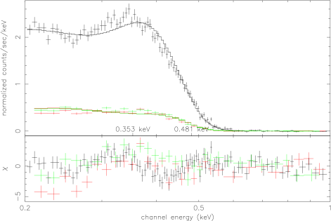
Figure 1: The background corrected count rate spectra of N LMC 1995 observed in the 0.2-1 keV energy range with XMM EPIC pn (in black) and EPIC MOS-1 and MOS-2 (respectively, in red and green) on December 19 2000. We also show the fit with model “b” and log(g)=8 (obtained simultaneously fitting the RGS data and excluding the range 0.2-0.3 keV for MOS data). In this NLTE atmosphere, we assume T_eff=407,000 K and N(H)=9 $\times$ 10²⁰ cm^-2.

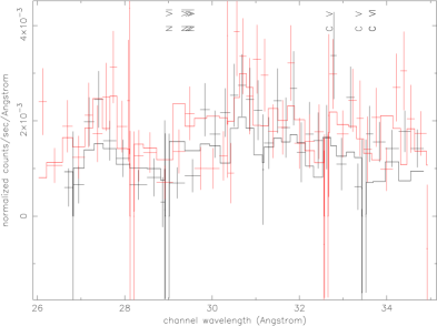
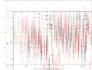
Figure 2: The panel on the top shows the background corrected count rate spectra of N LMC 1995 observed with XMM RGS-1 (in black) and with RGS-2 (in red) on December 19 2000 in the wavelength range 25-35 Å(energy range 0.353-0.481 keV). The best fit with model “b” (log(g)=8) to the spectrum observed with all the instruments (see Fig 1 and Table 3) is superimposed (folded with the response of both instruments). The panel on the bottom shows the residuals with each instruments at each wavelength. The wavelengths at which some of the strongest lines due to H-like and He-like transitions would be detected assuming a temperature 407,0000 K, are indicated.

We still detected the luminous supersoft X-ray source. The average count rates measured with the different instruments are shown in Table 1, and the observed EPIC and RGS spectra are shown in Fig. 1 and 2, respectively. The RGS energy range is 0.35-2.5 keV, and for N LMC 1995 there is no significant S/N above $\simeq$0.48 keV. The corresponding useful wavelength range is 26-35 Å. We indicated wavelength instead of energy in Fig. 2 to facilitate the comparison with Paerels et al. (2001), Bearda et al. (2001), and Burwitz et al. (2002).

We notice that this spectrum is peaked at lower energy than most supersoft X-ray sources, and can be compared only with the spectrum of nova V382 Vel observed with BeppoSAX 10 months after the outburst (Orio et al. 2002). In the case of V382 Vel, however, a low luminosity, hard component of nebular origin was also present, that is absent for N LMC 1995.

3.1 Time variability

The EPIC and MOS-1 background corrected lightcurves are shown in Fig. 3. The lightcurve background was extracted from a ring around the source and normalized to the extraction area used for the source. We rule out large flares (observed for V1494 Aql, see Starrfield et al. 2001, or Drake et al. 2002), or a sudden obscuration (observed for V382 Vel, see Orio et al. 2002). However, we found that the count rate varied by more than a factor of five during the $\simeq$46 ksec of observation. There are irregular variations on time scales of few minutes in the first portion of the light curve as well as a modulation with a longer time scale. The power spectrum shows the highest peak at 18900$\pm$100 seconds (5.25 hours), which is probably related to the orbital period (a study of the optical lightcurve is in preparation, Orio & Lipkin 2003). The modulation, which must be dependent on the inclination, is of larger amplitude than the X-ray eclipses observed for Cal 87 (Schmidtke et al. 1993), and possibly for GQ Mus (see Kahabka 1996; note that this result is uncertain because the orbital period of the system is close to the orbital period of the ROSAT spacecraft), but it is comparable to the one in the X-rays lightcurve of SMC 13 (Kahabka 1996). Other peaks found in the power spectrum are only aliases of the exposure time, and we did not detect the pulsations observed for V1494 Aql (Drake et al. 2002).

3.2 Comments on the RGS spectra

In Fig. 2 we show the portions of RGS spectra in the 25–35 Å range, for which the signal to noise ratio (S/N) is not too low for fitting model atmospheres. The wavelengths of the most important absorption lines in a thermal plasma at T$\simeq$407,000, obtained with the model fits (see Table 2), are labelled in the figure. At this temperature the he CNO elements must be in their H- and He-like charge states. Unfortunately, not only is the S/N ratio very modest, but the RGS does not have the spectral resolution (0.05 Å or less) needed to resolve most of the intricate line spectrum of an extremely hot white dwarf atmosphere.

However, these spectra are useful, also because the relative calibration of the two RGS is better determined than the EPIC calibration at the moment. For RGS-1 and RGS-2 the uncertainties in the relative calibration across the instruments are not greater than 7% and 5% respectively in the 20-28 Å range, and less than 12% and 10% in the 28-36 Å range. Moreover the RGS spectra, as it can be seen in in Fig. 2, also allow us to rule out the presence of strong, narrow lines in emission observed in the Chandra observation of Nova V382 Vel (due to the surrounding nebula, see Burwitz et al. 2002) and in the Chandra and XMM exposures of the supersoft X-ray source MR Vel (due to a wind, see Bearda et al. 2002 and Motch et al. 2002). We note that there is only one LMC supersoft source which is significantly brighter than N LMC 1995 in this spectral range, Cal 83, for which RGS count rate is $\approx$10 times higher, but this is partially due to the source being harder (Paerels et al., 2001). A qualitative comparison of the RGS spectra of N LMC 1995 and Cal 83 shows some similarities but also a large difference. The continuum for N LMC 1995 is fitted with atmospheric models with line opacities (see next section), but these models do not fit the continuum adequately for Cal 83 (Paerels et al. 2001). Not resolving the line spectra, detailed comparisons are not possible. Qualitatively, however, the RGS spectrum in the 25-35 Å  region appears quite different for Cal 83 and N LMC 1995.

3.3 Fitting white dwarfs atmospheric models to the observed spectra

The continuum of the EPIC spectra detected with the pn and the two MOS can be fitted with atmospheric models, to derive the white dwarf parameters and its chemical composition. The EPIC pn absolute calibration in the lowest energy range is still being improved. Before launch, the uncertainty in the relative calibration of EPIC-pn and EPIC MOS was only 1% in the 0.2-0.5 keV range. However, in the MOS the X-rays absorbed near the surface layers can loose a large fraction of their charge before collection, in a process which is not related to charge transfer inefficiency across the CCD (Breitfellner 2002, private communication). This effect is one of the dominating factors for the calibration and a large number of counts below 0.3 keV for sources with column density N(H)$\geq 10^{20}$ cm^-2 is due to scattered photons from higher energies. Extensive ground calibrations were used to construct a pre-flight response matrix, but after the launch the surface fractional charge loss at low energies was greater than observed on the ground. It also seems that the surface loss effect is not constant with epoch and observations of sky calibration sources after Orbit 300 reveal an excess of counts in the soft band. In a future release of the SAS software, the MOS calibration will be adjusted to incorporate the epoch dependent surface charge loss (Breitfellner 2002, private communication), but it is not available yet at present.

We used the XSPEC software package (Arnaud 1996). In the first two years after the outburst all novae seem to emit hard X-rays, but 6 years after the outburst, for this nova the 3 $\sigma$ upper limit to the X-ray flux in the range 0.6-10 keV is of $\simeq$10^-14 erg cm^-2 s^-1. The X-ray luminosity in this range is therefore L${}_{\rm x,hard}\leq 3\times 10^{33}$ erg s^-1. We remind that N Pup 1991 was still emitting a higher hard X-ray luminosity then this upper limit 16 months after the outburst (Orio et al. 1996).

For the emission below 0.6 keV, we find that the black-body in XSPEC is not adequate to explain the shape of the observed continuum. We used Local Thermodynamical Equilibrium (LTE) models of Heise et al. (1994), Non-LTE (NLTE) models developed by Hartmann & Heise (1997) and Hartmann et al. (1999), and also other metal enhanced NLTE atmospheric models developed by one of us (W.H.) for this project, and we implemented these models in XSPEC. Optically thick model spectra that only involve continuum opacities usually do not represent the observed spectrum correctly. We also included the effect of many line opacities (line blanketing), that change the temperature structure of the model atmosphere, therefore the ionization balance and eventually the shape of the model spectrum.

In our case, like for the observations done by other authors (e.g. Hartmann & Heise 1997), a better fit is definitely obtained with the NLTE models than with the LTE ones. The NLTE model atmospheres are calculated using the computer code TLUSTY (Hubeny 1988, Hubeny & Lanz 1995). This code uses the complete linearization technique to solve the coupled set of radiative transfer, radiative equilibrium and statistical equilibrium equations. Convergence is achieved when the relative changes of the temperature, total number density and electron density are smaller than 10^-3. For a detailed description of the computer code TLUSTY we refer to Hubeny (1988) and Hubeny & Lanz (1995).

Lanz & Hubeny (1995) show that metal line opacities for carbon and iron have to be taken along in NLTE model atmosphere calculations. They conclude that line blanketing by trace elements with abundances above solar influences the atmospheric structure of hot, metal-rich white dwarfs. Rauch (1996) calculated line-blanketed NLTE model atmospheres, to show that light metal opacities drastically decrease the flux levels of hot stars. We restrict ourselves to a limited number of ionization stages and atomic levels. The spectrum of hot, high-gravity atmospheres is often dominated by the lowest levels of one or two ionization stages of a particular element. Therefore, we selected the ionization stages that we expected to be most dominant in the range of parameters of interest. Table 2 shows the ionization stages included for the ions of the elements considered (H, He, C, N, O, Ne, Mg, Si, S, Ar, Ca, and Fe). The atomic data are from the Opacity Project Database (Cunto et al., 1993). We refer to Hartmann et al. (1999) for the detailed treatment of continuum opacities.

To fit the N LMC 1995 XMM spectra, we tested a grid of models for log(g)=8, 8.5, 9, interpolating between temperature steps of 50,000 K, with the following sets of abundances:

a) cosmic abundances (Anders & Grevesse 1989);

b) “LMC-like” abundances, (from Dennefeld, 1989, roughly 0.25 times the cosmic values);

c) C, N and O enhanced by a factor of 10 with respect to “cosmic”;

d) Ne, O and Mg enhanced by a factor of 10;

e) enhanced He (H/He=0.5 in number abundance) and enhanced C/N ratio (a model atmosphere developed for U Sco, see Kahabka et al. 1999).

We adopted the strategy of fitting the data of the different instruments separately at first, then we combined the EPIC pn and MOS spectra. Finally, we fitted the spectra of all 5 instruments together. We examined and fitted the the RGS spectra only in the range 0.35-0.48 keV (26–35 Å), where the signal to noise ratio is large, but still acceptable, because the rest of the spectrum is too noisy. In Table 3 we report all the results of spectral fits that yielded $\chi^{2}$/d.o.f. $\leq$ 1.5. No models fit the MOS spectra with $\chi^{2}$/d.o.f. $\leq$ 1.6 if we include the range 0.2-0.3 keV. We attributed this to a difference in the relative calibration of the MOS and pn at this energy, probably due to the surface layers absorption mentioned above. Since fitting the pn spectrum at 0.2-1 keV decreases $\chi^{2}$/d.o.f. a little, but the qualitative results agree quite well with the results in the 0.3-1 keV range (see Table 3), we tried including the 0.2-0.3 keV range for the pn. When we did, we obtained a higher value of the equivalent column of neutral hydrogen, N(H). We set some limits inside which we accept that the N(H) parameter may vary: N(H)=0.7–1.8 $\times$ 10²¹cm^-2, from the Galactic absorption to the LMC, to this value plus the intrinsic absorption in the LMC, evaluated with Points’ (2002) ATCA-Parkes H I maps (which show that the N(H) column all the way to the back of the LMC in the direction of the nova is 1.1 $\times$ 10²¹ cm^-2.)

The best fit T_eff and N(H) with their 2 $\sigma$ uncertainties are given in Table 3, for models which yield $\chi^{2}$/d.o.f.$\leq$1.5. The value of T_eff varies in a narrow range in all the models and the uncertainties on the absorbed flux typically do not exceed 25%. The last two columns of Table 3 indicate the parameters that we used to determine what model fits the spectrum. One parameter is $\chi^{2}$/d.o.f. (last column). The column before the last lists also the other important parameter that we had to consider: the normalization factor K = (R_WD/d)², where d is the distance to the LMC (here we adopted 51 kpc, but a distance of 55 kpc, adopted by other authors, does not change our general conclusions). Deriving the radius R_WD from K, we obtain the white dwarf mass M_WD knowing the effective gravity g (which is a model characteristic) through M_WD = g R${}_{\rm WD}^{2}$/G . The normalization factor K must indicate a mass M_WD in the range 0.6–1.4 M_⊙. All models with a value of “K” that yields M_WD outside this range are not consistent with the LMC distance. The upper limit is the Chandrasekhar mass, the lower one the minimum mass to obtain a sufficient density in the shell to allow thermonuclear burning of hydrogen. At very high effective temperature, for the hydrogen burning shell to radiate all the energy it produces, R_WD must be bloated to some extent. It may be quite larger than the Chandrasekhar radius (e.g. Prialnik 1986, MacDonald et al. 1985). We note that the value of K increases dramatically with N(H), but keeping constant N(H), K increases also with the effective gravity. N(H) and K, unlike the temperature and the absorbed flux, vary by a large extent for the different models.

All the atmospheric models with enhanced carbon, either in LTE or NLTE (specifically models “c” or “CNO enhanced” and “e” or U Sco-like), are not included in Table 3 except in one case for the RGS, because they cannot fit the EPIC data. This is mainly due to a too deep absorption edge of C VI at 0.49 keV. Therefore, we find that carbon is not enhanced. The continuum predicted by model “e” differs mostly from the observed continuum, and this is due mainly to the enhanced C/N ratio (more than to the helium enhancement).

Regardless of the value of the “K” normalization factor, the best fit to the EPIC pn spectra and to all the instruments simultaneously, is obtained with the NLTE model atmosphere “d” with log(g)=9, at T${}_{\rm eff}\simeq$ 450,000 K, and N(H) = 1.6 $\times 10^{21}$ cm^-2. This model fits the data better due to a deeper edge of Mg X at 0.347 keV, and one of Mg IX at 0.23 keV, which affect the continuum slope at low energy. Thus is it is possible that magnesium is enhanced, but the fit had to be discarded due to the value of the constant K, which is definitely too high. This model indicates a high column density N(H) and so high a flux that the white dwarf mass would exceed the Chandrasekhar mass by a great amount. The same is true even for the second best fit, the same model with log(g)=8.5. Model “d” with log(g)=8 does not fit the EPIC spectra adequately. Even if the next good model, “b” with log(g)=8, fits the spectrum a little less well (especially due to a poorer result if we include the spectral range 0.2-0.3 keV for the EPIC pn) the constant K is finally acceptable. The value of K for the best fit to all the instruments, including the 0.2-0.3 keV range of the pn, indicates M_WD = 0.905 M_⊙. The unabsorbed flux in the 0.2-1.0 keV band is F${}_{\rm x}=8\times 10^{-13}$ erg cm^-2 s^-1, and the bolometric luminosity is L${}_{\rm bol}=2.3\times 10^{37}$ erg s^-1 at a distance 51 kpc.

We note that all the fits with the atmospheric models, in LTE and NLTE, for all instruments, indicate 3.9 $\times 10^{5}\leq$ T${}_{\rm eff}\leq 4.7\times 10^{5}$ K, but the RGS spectra are always best fitted with T${}_{\rm eff}>4\times 10^{5}$ K. Comparing with the results for the PSPC data in Orio & Greiner (1999), this clearly indicates that the WD atmospheric temperature has remained at least constant (within the 2$\sigma$ confidence level) or, most probably, has increased.

A post-nova white dwarf which is still burning hydrogen in a shell is expected to evolve at constant bolometric luminosity. While the radius shrinks and the atmosphere becomes hotter, the flux in the 0.2-1 keV range is supposed to remain constant. An unabsorbed bolometric flux F_bol of order of $\simeq$5 $\times 10^{-10}$ erg cm^-2 s^-2, was consistent with the fit of Orio & Greiner (1999; note that the fit was done with models at fixed bolometric luminosity, unlike the models used here for which the normalization constant is a parameter). This is an order of magnitude larger than F_bol we derived here, but we have to stress that the 1$\sigma$ uncertainty in the ROSAT spectral fit parameters translates in an uncertainty of more than one order of magnitude in the flux, so we ignore whether the peak temperature was reached between the ROSAT and the XMM-Newton observations and whether the flux at the end of 2000 had started to decrease. The models used in Orio & Greiner (1999) are LTE models of MacDonald & Vennes (1991). The white dwarf in the model had log(g)=7 and R_WD=2.5 $\times 10^{10}$ cm. The white dwarf radius is only R_WD=1.09 $\times 10^{9}$ cm in our “b” model with log(g)=8. Despite the different models used, clearly the evolutionary picture that emerges is that of a shrinking atmospheric radius in the period from the beginning of 1998 and the end of 2000, and it is consistent with the theoretical prediction.

4 Conclusions

The spectrum of the post-nova supersoft X-ray sources in the first year or two after the outburst can be very complex. The X-ray flux in other novae around one year after the outburst has been observed to vary dramatically on short time scales, and this is not well understood yet (Orio et al. 2002, Drake et al. 2002). The central source may be hidden by another source of X rays, thought to be the ejected nebula, with emission lines in the supersoft X-ray range due to transitions of highly ionized elements. These narrow emission lines were resolved only in one case with the Chandra LETG (Burwitz et al. 2002, see also the discussion of Orio et al. 2002). Since the BeppoSAX LECS and the ROSAT PSPC could not resolve super-imposed nebular narrow emission lines from the central source spectrum, temperature and effective gravity determined from the observations of V1974 Cyg (Balman et al. 1998) and of V382 Vel (Orio et al. 2002) should be considered very uncertain. N LMC 1995, at the late post-outburst stage at which it was observed, appears as a “simpler” source, without nebular emission. Grating observations of another supersoft X-ray source have also shown narrow emission lines, most likely due to an ongoing stellar wind that emits X-rays and shields the white dwarf continuum, (Bearda et al. 2002). These lines are also absent for Nova LMC 1995. Moreover, despite some variability (probably connected with the orbital period), sudden flares or obscurations are not observed. Thus this nova offers a rare, perhaps unique opportunity to observe the “naked” atmosphere of a supersoft X-ray nova remnant and determine the white dwarf parameters. We consider it a sort of “Rosetta stone” of hydrogen burning, post-outburst novae. Once the EPIC calibration is refined, and the epoch-dependent MOS calibration is made available, it will be meaningful to try and fit the spectra with a finer grid for log(g). The important point is that, if we determine log(g) more accurately, we also obtain a precise estimate of M_WD. We remind that we have not yet included detailed NLTE models with log(g)=7.5, which still have to developed, but since there is a clear trend of K with log(g), we foresee that for LMC abundances we would obtain too low a mass. On the other hand, models with higher abundances, with the present instrument calibration do not fit the data with a reasonable value of K for any value of log(g).

A different, but model-dependent way in which we may derive the white dwarf mass, will be to measure the atmospheric temperature reached at maximum. According to all models (e.g. MacDonald et al. 1985), this temperature it is critically dependent on the white dwarf mass. For this reason, we have required further monitoring with XMM-Newton, and it has been scheduled for 2003. There is also an inverse dependence of the white dwarf mass on the time to reach the peak temperature. According to the relationships given by MacDonald et al. (1985), the range of masses for which the peak effective temperature is expected to exceed T${}_{\rm eff}\geq$407,000 K (yielded by our most likely model “b”), yet the time during which this temperature increases is $\geq$ 6 years, is 0.74 M${}_{\odot}\leq$ M${}_{\rm WD}\leq$ 1.21 M_⊙, in agreement with the best estimate M $\simeq$ 0.9 M_⊙ derived from the model atmosphere. MacDonald et al. (1985) predict that a white dwarf of 0.9 M_⊙ burns hydrogen in a shell for almost 39 years, exceeding a maximum temperature of 550,000 K, which will be reached slowly while the atmosphere shrinks. The new observations, done again with XMM, and the improved EPIC calibration, should allow us to verify this theoretical prediction by measuring the white dwarf mass in two independent ways: with model atmospheres, and deriving it from the peak temperature and turn off time. This will be an important test for the models.

We tested atmospheric models with different abundances. If there is significant mixing with the white dwarf material, slowly “eroded” during the secular evolution, the white dwarf (which presumably is a CO or a Ne-O-Mg white dwarf) may be burning some of its own material (not accreted from the companion), and be decreasing rather than increasing in mass. With the present status of instrument calibration, we were only able to determine that carbon is not significantly enhanced. If there is mixing with the outer layers of a CO white dwarf, both these two elements would be enhanced, but the carbon abundance is the one that mostly produces a change in spectral shape in the energy range in which N LMC 1995 emits copious flux. This change has not occurred. The spectral fits and the distance constraints seem to even favor a model with depleted abundances, but an improved instrument calibration will be necessary to better assess the sophisticated differences in the models and perhaps find out whether the burning material may be accreted from the companion. Since shell hydrogen burning has continued immediately after the outburst, if the hydrogen rich material is not significantly enhanced in heavy elements it cannot have its origin in the WD itself, but it must be accreted material, still retained after the eruption.

This is important because, if the white dwarf mass grows, after repeated nova outbursts it might reach the Chandrasekhar mass and explode as type Ia SN. However, we have no indications that M_WD in N LMC 1995 is anywhere near the Chandrasekhar value yet. If M${}_{\rm WD}<<1.4$ M_⊙, it could take longer than the Hubble time. Another scenario in which a nova systems eventually undergoes a type Ia SN explosion is a “sub-Chandrasekhar mass” model (see Fujimoto & Sugimoto 1982) in which, after many nova outbursts, the supernova explosion is triggered by a helium flash. The helium flash is made possible by significant accumulation of a helium buffer during previous hydrogen burning in the nova secular evolution. In this work we could not prove, nor definitely rule out that the burning layer already shows significantly enhanced helium. We suggest that this should be assessed in the future with observations at other wavelengths, for instance detecting the He II $\lambda$1640 absorption line in the ultraviolet spectrum when the white dwarf is cooling.

One other interesting question remains open. What is the difference between a classical nova like N LMC 1995 and GQ Mus, that burns hydrogen in a shell for several years after the outburst, and the majority of novae, for which turn off occurs within a couple of years? Ögelman et al. (1993) speculated that for GQ Mus hydrogen burning is rekindled because of irradiation induced mass transfer from the companion. This mechanism, however, is efficient for systems with orbital periods shorter than 4 hours (Kovetz et al. 1988), but it does not seem to operate efficiently when the orbital period, like probably in this nova, is larger (Lipkin & Orio 2003, in preparation). The theoretical models foresee that the white dwarf mass is the main parameter that determines the turn-off time and the amount of accreted mass retained after each outburst. We hope to verify it, thus answering one of the most basic questions of nova physics, by monitoring the further evolution of N LMC 1995 in X-rays, and possibly at the same time in optical and ultraviolet.

                 

                                                 

                 

Figure 3: The EPIC-pn and EPIC-MOS-1 background corrected light curves during the observation, binned every 200 s.

Table 1: Average background corrected count rates measured with the Newton-XMM instruments.

Instrument	Range (keV)	Count rate (cts s-1)
EPIC pn	0.2-10	0.5754$\pm$0.0043
EPIC MOS-1	0.2-10	0.1025$\pm$0.0017
EPIC MOS-2	0.2-10	0.1144$\pm$0.0017
RGS-1	0.3-3.5	0.0196$\pm$0.0010
RGS-2	0.3-3.5	0.0221$\pm$0.0010

Table 2: Species of ions, number of levels considered, their main quantum number, number of lines used in the preliminary atmosphere calculation with temperature 400,000 K, number of lines used in the spectrum calculation between 20 and 40 Å (see Hartmann et al. 1999 for details). Note that the exact number of lines in the spectrum varies with T_eff.

Ion	Levels number	Quantum number	Lines (atmosphere)	Lines (spectrum)
HI	9	1-9	28	0
HeII	14	1-14	78	0
CV	5	1-2	3	8
CVI	6	1-3	5	9
NV	5	2-3	6	0
NVI	5	1-2	3	9
NVII	6	1-3	5	2
OVI	5	2-3	6	0
OVII	5	1-2	3	1
NeVIII	5	2-3	6	0
NeIX	5	1-2	3	0
MgX	5	2-3	6	48
Mg XI	5	1-2	3	40
SX	8	2	9	429
SXI	12	2	12	611
SXII	8	2	9	391
SXIII	6	2	4	158
ArX	2	2	1	91
ArXI	6	2	4	353
ArX	2	2	1	91
ArXI	6	2	4	353
ArXII	8	2	9	676
CaX	7	3-4	11	0
CaXI	15	2-3	20	18
CaXII	12	2	1	84
FeXV	14	3	19	206
FeXVI	7	3-4	11	24
FeXVII	15	2-3	20	382
Fe XIV	6	3	4	284

Table 3: Parameters of the NLTE atmospheric models (described in the text) fitted to the observed spectra, for models which yield $\chi^{2}$/d.o.f.$\leq$1.5 at least in the 0.3-1.0 spectral range. Best fit temperature and column of neutral hydrogen N(H) (given with the 2$\sigma$ error unless N(H) if it was “frozen”, in which case it is marked with an asterisk), and normalization constant K=R${}_{\rm WD}^{2}$/d². The flux was multiplied by a constant, normalized to 1 for the pn, and let vary as a free parameter for the other instruments. It turned out to be about 1.05 for MOS-1, 1.15 for MOS-2, 0.65 for both two RGS, respectively. The spectrum was always fitted above 0.3 keV for the two MOS, in the range 0.35-0.48 keV for the two RGS, and if the pn is included in the fit, the “range” reported in column 2 is for the pn.

Instrument	range	Model	log(g)	T${}_{\rm eff}\times 10^{3}$	N(H) $\times 10^{21}$	K $\times 10^{-29}$	$\chi^{2}$/d.o.f.
	(keV)			(K)	(cm-2)
pn	0.3-1.0	b	8.0	411$\pm$1	0.70$\pm$0.04	2.59	1.38
pn	0.3-1.0	d	8.0	402$\pm$1	1.80*	341.99	1.07
pn	0.3-1.0	d	8.5	452$\pm$2	1.09$\pm$0.13	24.97	1.10
pn	0.3-1.0	d	9.0	454${}^{+8}_{-7}$	1.48$\pm$0.13	70.86	0.99
pn	0.3-1.0	d	8.5	454$\pm$2	1.09$\pm$0.13	24.97	1.10
pn	0.2-1.0	d	8.5	452${}^{+1}_{-6}$	1.41${}^{+0.06}_{-0.04}$	48.54	1.33
pn	0.2-1.0	d	9.0	452${}^{+2}_{-5}$	1.57${}^{+0.08}_{-0.06}$	91.33	1.09
MOS	0.3-1.0	a	9.0	417$\pm 6$	1.80*	321.66	1.29
MOS	0.3-1.0	b	9.0	399${}^{+1}_{-14}$	1.80*	57.19	1.26
MOS	0.3-1.0	d	8.5	446${}^{+5}_{-14}$	1.48${}^{+0.08}_{-0.07}$	84.28	1.40
pn + MOS	0.3-1.0	b	8.0	411$\pm$2	0.70$\pm$0.05	2.84	1.07
pn + MOS	0.2-1.0	d	8.5	451$\pm 1$	1.45${}^{+0.04}_{-0.05}$	54.45	1.40
pn + MOS	0.2-1.0	d	9.0	451${}^{+1}_{-4}$	1.64${\pm 0.07}$	113.45	1.27
RGS	0.35-0.48	b	8	410$\pm$6	0.70*	2.23	1.28
RGS	0.35-0.48	d	8	402${}^{+9}_{-7}$	1.34${}^{+0.15}_{-0.50}$	165.19	1.41
RGS	0.35-0.48	d	8.5	454${}^{+9}_{-4}$	0.75$\pm 0.12$	10.83	1.40
RGS	0.35-0.48	d	9.0	477${}^{+23}_{-18}$	0.69$\pm 0.34$	6.24	1.25
RGS	0.35-0.48	e	8.0	416${}^{+7}_{-5}$	0.70*	0.75	1.28
RGS	0.35-0.48	e	8.5	460${}^{+38}_{-4}$	0.74${}^{+0.13}_{-0.05}$	0.40	1.33
RGS	0.35-0.48	e	9.0	473$\pm 15$	1.18$\pm$0.35	0.74	1.37
pn + RGS	0.3-1.0	b	8.0	411$\pm 2$	0.70*	2.58	1.17
pn + RGS	0.2-1.0	b	8.0	407$\pm 2$	0.90$\pm$0.02	4.87	1.53
pn + RGS	0.2-1.0	d	8.5	452${}^{+1}_{-7}$	1.41$\pm 0.05$	49.60	1.38
pn + RGS	0.2-1.0	d	9.0	453$\pm$2	1.54${}^{+0.06}_{-0.02}$	83.82	1.27
ALL	0.3-1.0	b	8.0	409$\pm$1	0.70*	2.75	1.30
ALL	0.2-1.0	d	8.5	451${}^{+2}_{-7}$	1.46$\pm$0.05	53.9	1.42
ALL	0.2-1.0	b	8.0	407$\pm$2	0.90$\pm$0.02	4.87	1.53
ALL	0.2-1.0	d	8.5	451${}^{+1}_{-7}$	1.45$\pm$0.05	54.48	1.41
ALL	0.2-1.0	d	9.0	451$\pm$1	1.60$\pm$0.08	102.39	1.35