Beyond the Hubble Deep Field limiting magnitude: faint galaxy number counts from surface-brightness fluctuations

Abstract

The faint end of the differential galaxy number counts, $n(m)$, in the Hubble Deep Field (HDF) North has been determined for the F450W, F606W, and F814W filters by means of surface-brightness fluctuation (SBF) measurements. This technique allows us to explore $n(m)$ beyond the limiting magnitude of the HDF, providing new, stronger constraints on the faint end of $n(m)$. This has allowed us to test the validity of previous number count studies and to produce a new determination of the faint end of $n(m)$ for magnitudes fainter than $28.8$ in the $AB$ system and to extend this estimate down to $31$. This value represents an extension of more than two magnitudes beyond the limits of previous photometric studies. The obtained $n(m)$ slopes are $\gamma=0.27$, $0.21$, and $0.26$ in $B_{450}$, $V_{606}$, and $I_{814}$, respectively.

1 Introduction

The galaxy luminosity function ($\Phi$) remains at the core of both galaxy evolution and cosmology. By integrating $\Phi$ over space and time, various observable distributions can be obtained. In particular, differential number counts of galaxies as a function of apparent magnitude, $n(m)$, is obtained by integrating $\Phi$ over all redshifts and morphological types. The reliability of the predicted $n(m)$ values depends directly on the cosmological model and on how well the evolution of galaxies is modelled from their formation to the present. The study of number counts can therefore be used to test world models or to search for evolution during the look-back time.

The function $n(m)$ provides one of the most fundamental observables and has been studied by several authors (for reviews see Ellis 1997; Koo & Kron 1992; Sandage 1988). Recently, a major effort has been made to reach very faint magnitudes using the Hubble Space Telescope (HST). Although the HST cannot compete with ground-based observations in terms of collecting area, it does provide an unprecedent view of the optical sky at small angular scales and faint flux levels. A number of authors have studied faint galaxy counts based on the Hubble Deep Field (HDF) (Williams et al., 1996) and using different photometry packages (Williams et al., 1996; Metcalfe et al., 1996; Lanzzetta, Yahil, & Fernández-Soto, 1996; Pozzetti et al., 1998; Metcalfe et al., 2001). In this paper, we use the notation $B_{450}$, $V_{606}$, and $I_{814}$ to denote magnitudes in the HST passbands on the $AB$ system (Oke, 1974). Ferguson (1998) has compared the HDF catalogues available in the literature. They generally show good agreement, although the effects of different isophotal thresholds and different splitting algorithms are apparent. However, Ferguson, Dickinson, & Williams (2000) showed that, at $I_{814}=26$, the different galaxy counts agree to within $25\%$ in all the catalogues, whereas at $I_{814}=28$ there is a factor of 1.7 difference among them. This emphasizes the fact that galaxy counting is not a precise science.

In this paper, the HDF will be used to test the validity of previous number count studies and to produce a new determination of the faint end of $n(m)$ for magnitudes fainter than $28.8$. Surface-brightness fluctuation (SBF) measurements are used. This allows us to explore $n(m)$ beyond the limiting magnitude of the HDF and to overcome most of the limitations arising from incompleteness, providing new, stronger constraints on the faint end of $n(m)$.

2 The data

This work is based on data from the HDF North. Observations were made in 1995 December 18–30, and both raw and reduced data have been put into public domain as a community service (Williams et al., 1996). Version 2 F450W, F606W and F814W images, released into public domain on 1996 February 29, have been used here.

The final Version 2 images were combined using the DRIZZLE algorithm. Drizzling causes the noise in one pixel to be correlated with the noise in the adjacent one (Williams et al., 1996). The SBF technique is based on the spectral analysis of an image. Because the power spectrum of the image is modified by the drizzling process, drizzled images were not considered in this study. “Weighted and cosmic-ray cleaned” images have been used instead. These are flat-fielded, cosmic-ray-rejected and sky-subtracted stacked images at each dither position. Only dark exposures have been selected. Each of the the three wide-field and the planetary camera WFPC2 chips were analyzed separately. The labels of all images considered, the corresponding filter and the total exposure times are listed in table 1.

3 Surface-Brightness fluctuations in the HDF-N

The SBF concept was introduced by Tonry & Schneider (1988), who noted that, in the surface photometry of a galaxy far enough away to remain unresolved, a pixel-to-pixel fluctuation is observed because of the Poisson statistics of the spatial distribution of stars, globular clusters, background galaxies, etc. This technique was introduced with the aim of measuring distances. Comparing SBFs produced by the stellar population of a galaxy with those of nearby galaxies for which externally calibrated distances are available, accurate estimates of distances can be obtained up to $\sim$40 Mpc (Tonry et al., 2000, 2001). Other authors have used SBF studies to determine the age and metallicity of unresolved stellar populations of nearby galaxies (Liu, Charlot, & Graham, 2000; Blakeslee, Vazdekis, & Ajhar, 2001; Hidalgo, Marín-Franch, & Aparicio, 2003); however, the SBF signal can provide information about other kinds of undetected and unresolved objects in an image. This is the case, for example, of globular cluster populations (Blakeslee & Tonry, 1995; Blakeslee, 1999; Marín-Franch & Aparicio, 2002, 2003). In this paper, SBFs have been used to characterize the faint end of $n(m)$ using undetected galaxies in the HDF-N images.

Next in this section, the theoretical background of SBFs and the HDF-N signal measurement are described in detail.

3.1 Theory

The SBF technique involves spectral analysis of the pixel-to-pixel fluctuation signal. This provides the total point spread function PSF-convolved variance ($P_{0}$) produced by all point objects whose spatial flux distribution is convolved with the PSF, and the total non-PSF-convolved variance ($P_{1}$). A convolution in the real space transforms into a product in Fourier space. For this reason, the power spectrum of an image, $P(k)$, has the form:

$$P(k)=P_{1}+P_{0}E(k),$$ (1)

where $E(k)$ is the power spectrum of the PSF convolved with some window function. The $E(k)$ can be approximated by the power spectrum of the PSF alone, $P_{\rm PSF}(k)$, with a negligible error (Jensen et al., 1998). So eq. 1 transforms into

$$P(k)=P_{1}+P_{0}P_{\rm PSF}(k).$$ (2)

Once the power spectrum of an image has been computed, the variances $P_{0}$ and $P_{1}$ can be obtained fitting eq. 2 to data.

In HDF images, $P_{0}$ is mainly produced by faint galaxies, and, as we will see later, by cosmic rays. So $P_{0}$ must be equal to the sum of the variances produced by faint galaxies ($\sigma^{2}_{\rm BG}$) and by cosmic rays ($\sigma^{2}_{\rm cr}$):

$$P_{0}=\sigma^{2}_{\rm BG}+\sigma^{2}_{\rm cr}.$$ (3)

On the other hand, $P_{1}$ is the sum of read-out noise ($\sigma^{2}_{\rm ro}$), photon shot noise ($\sigma^{2}_{\rm ph}$), and dark current ($\sigma^{2}_{\rm dc}$) variances:

$$P_{1}=\sigma^{2}_{\rm ro}+\sigma^{2}_{\rm ph}+\sigma^{2}_{\rm dc}.$$ (4)

The pixel-to-pixel variance produced by a class of objects can be evaluated as the second moment of the differential number counts of that object population (Tonry & Schneider, 1988). In the present study, the target population is composed by faint undetected galaxies. The brightest individuals, which are detected, must be masked out before the SBF analysis. If all sources brighter than a limiting flux ($f_{\rm lim}$) are masked, then the variance produced by the remaining non-masked population is:

$$\sigma^{2}_{\rm BG}=\int_{0}^{f_{\rm lim}}n(f)f^{2}df.$$ (5)

We can put this equation in terms of magnitudes via the relationship

$$m=-2.5\log(f)+m^{*}_{1},$$ (6)

$f$ being the flux ($DN$ s^-1 pix^-1), and $m^{*}_{1}$ the magnitude of an object yielding one unit of flux per unit time; that is, the photometric zero point listed in Table 2.

If $n(m)$ is known, then the theoretical variance produced by faint galaxies can be estimated. Assuming the following pure power-law form for $n(m)$:

$$n(m)=A_{0}10^{\gamma m},$$ (7)

where $A_{0}$ is a normalizing constant and $\gamma$ is the slope of the magnitude distribution, the variance produced by the non-masked galaxy population is then

$$\sigma_{\rm BG}^{2}=\frac{A_{0}}{\ln 10(0.8-\gamma)}10^{\gamma m_{\rm c}}10^{0.8(m_{1}^{*}-m_{\rm c})},$$ (8)

where $m_{\rm c}$ is the limiting magnitude; i.e. the magnitude corresponding to the limiting flux, $f_{\rm lim}$. We will refer to this variance as the $n(m)$-estimated $\sigma_{\rm BG}^{2}$ from here on. As we have shown, in order to compute it, an initial $n(m)$, obtained from a given photometric catalogue, must be assumed.

3.1.1 Photometric catalogues

A number of authors have studied $n(m)$ in the HDF-N. The main discrepancies between previous number count studies occur between Williams et al. (1996) and Metcalfe et al. (2001). These coincide for “bright” magnitudes, but large differences arise for fainter galaxies, the Metcalfe et al. (2001) number counts being larger than those of Williams et al. (1996).

As pointed out by Ferguson (1998), there are two reasons for this discrepancy. First, as we go fainter the Metcalfe et al. (2001) magnitudes become systematically brighter than those of Williams et al. (1996). Metcalfe et al. (2001) claimed that the effect of this on the counts is actually quite small, generally $<10\%$. Second, Metcalfe et al. (2001) find objects that Williams et al. (1996) do not detect at all. This appears to account for the majority of the differences between the data sets. Metcalfe et al. (2001) argued that virtually all of these objects are merged in the reductions of Williams et al. (1996) but not in their data.

In Figure 1, differential number counts results from Williams et al. (1996) (filled circles) and Metcalfe et al. (2001) (open circles) are plotted for the F450W, F606W, and F814W filters, respectively. These data have been obtained from tables 9 and 10 in Williams et al. (1996), and from tables 8, 10 and 12 in Metcalfe et al. (2001), all expressed in the total magnitude scale. Following eq. 7, $n(m)$ has been fitted to the data of Williams et al. (1996) and Metcalfe et al. (2001), and the fitted functions (solid lines) are also plotted. As Williams et al. (1996) found a change in the $n(m)$ slope at a magnitude of around 26, $n(m)$ has been fitted to their data in the two magnitude intervals [23, 26] and [26, 29].

The fitted $n(m)$ functions have been used in eq. 8 to compute the $n(m)$-estimated $\sigma_{\rm BG}^{2}$. Results are listed in table 3. These $n(m)$-estimated $\sigma_{\rm BG}^{2}$ values will be later on compared with those directly derived from the SBF measurements (which we will call the SBF-measured $\sigma_{\rm BG}^{2}$). This comparison will allow us to evaluate the validity of the differential number counts of both Williams et al. (1996) and Metcalfe et al. (2001) and, as a result, a final $n(m)$ will be proposed.

Before describing the details of the SBF measurements in HDF images, note that the SBF technique is valid only if faint galaxies have a stellar appearance. In Ferguson (1998) the radius–magnitude relation for galaxies in the Williams et al. (1996) HDF catalogue has been analyzed. For magnitudes fainter than $V_{606}=28.8$, all the galaxies have a radius smaller that $0.16\arcsec$, close to the FWHM of the WF chips. So very faint galaxies, in the magnitude range where SBF will be measured, can be assumed to have a stellar appearance.

3.2 Procedure to obtain SBF

Here, the practical procedure for obtaining the SBF signal in HDF-N images is described in detail. First of all, it should be noted that cosmic rays are difficult to discriminate from stars in HST frames. In order to estimate and eliminate the cosmic-ray contribution to the SBF signal, $P_{0}$, a procedure based on the random nature of cosmic-ray events has been used for each filter and chip. The SBF signal has be measured not only on the final combined images, but on all the individual images listed in Table 1 as well.

Before computing the power spectrum of an image, objects brighter than $m_{\rm c}$ must be masked out. In this study, the window functions have been created using the Williams et al. (1996) photometric catalogue, which is the only one available to us. As isophotal magnitudes were considered while creating the window functions, in order to convert them to the total magnitude scale an isophotal-to-total magnitude correction of 0.2 mag (Williams et al., 1996) was applied. The SBF analysis have been be performed considering two different values of $m_{\rm c}$: 27.8 and 28.8. All objects brighter than $m_{\rm c}$ have been masked out using a window function whose pixel values are zero in a circle centered on the location of the bright objects and unity in the rest of the image. The window function has been created using a patch radius large enough to completely mask bright galaxies, including their external haloes and therefore merged galaxies where these exist. The procedure creating the mask has been the following: first, the brightest galaxies have been masked one by one manually. In order to avoid residual light beyond the masked regions, very generous patch sizes have been adopted. The shape of the used patchs for these very bright galaxies depends on the shape of the particular masked galaxy. Once bright galaxies have been masked, the rest of galaxies brighter than the chosen $m_{\rm c}$ have been masked using circular patches. The radius of these patches has been chosen to be the same for all galaxies, and its size is again very generous: the adopted patch radius is 15 pixels.

In order to test if all the residual light beyond the masked regions has been eliminated, the SBF analysis has been repeated for one image varying the radius of the patches. We have considered patch radii of 20, 25 and 30 pixels. Note that if a radius larger than 30 pixels would be used, the image would be completely masked due to the superposition of adjacent patches. The considered image has been the F450W average image of WF2 with $m_{c}=27.8$. The SBF results are listed in table 4. It can be seen that the SBF results are independent of the patch radius. As a conclusion, it can be seen that the adopted patch radius avoid residual light beyond the masked regions, as required.

If the differences between the Williams et al. (1996) and Metcalfe et al. (2001) data sets relies on the objects that are merged in the former and not in the latter, as argued by Metcalfe et al. (2001), then the created window function is virtually the same as one would obtain using the Metcalfe et al. (2001) photometric catalogue, and also masks objects that are in this catalogue and not in that of Williams et al. (1996).

Next, multiplying the window function by the image, the residual masked image is obtained. It is this image which is used to compute the power spectrum. As has been said, two sets of masked images have been computed, one for each $m_{c}$ value.

The power spectrum of the masked image is two-dimensional. It is radially averaged in order to obtain the one-dimensional power spectrum. Fitting the power spectrum of the images with eq. 2, the quantities $P_{0}$ and $P_{1}$ can be obtained for each image. As we could not construct a PSF from HDF images, since there were not enough stars in any of the four chips, the used PSFs were the high-S/N PSFs extracted by P. B. Stetson from a large set of uncrowded and unsaturated WFPC2 images.

Spatial variations of the PSF along the CCD mosaic could introduce a significant uncertainty in $P_{0}$. To limit this effect, we have used a PSF template for each one of the four chips of the WFPC2. Minor PSF variations inside each particular chip have not been considered. For each chip, both PSF and the computed power spectrum represent mean values across the complete field of the chip, so any spatial variation of the PSF across the chip would affect the SBF fitting procedure, introducing an uncertainty in the $P_{0}$ measurement. This uncertainty is small, and in any case, it is included in the obtained $P_{0}$ uncertainty.

In Fig. 2 we show an example of the SBF fitting procedure in an HDF image. The observed discrepancy at low wave numbers between the obtained power spectrum and the fit is due to large scale fluctuations in the background brightness of the images. This wave number region, where the discrepancy occurs, is not taken into account when fitting eq. 2. The power-spectrum fitting procedure is the following: eq. 2 is used to fit the power spectrum for wave numbers in the range [$k_{0}$, $k_{\rm max}$], $k_{\rm max}$ being the highest wave number of the computed power spectrum, and $k_{0}$ a number which we vary from 0 to $k_{\rm max}$. As a result, two functions, $P_{0}(k_{0})$ and $P_{1}(k_{0})$, are obtained. The function $P_{0}(k_{0})$ is also shown in Fig. 2 (small boxes). It can be seen that this function exhibits a “plateau” region. The final adopted result and its uncertainty for $P_{0}$ are obtained computing the average and standard deviation of $P_{0}(k_{0})$ in the plateau interval. For the $P_{1}$ measurement, the procedure is exactly the same as for $P_{0}$.

$P_{0}$ and $P_{1}$ results corresponding to $m_{c}=27.8$ and $m_{c}=28.8$ are listed in Tables 5 and 6, respectively. Results are listed for all images, corresponding to all chips and all filters.

4 Results

In this section, results from Tables 5 and 6 will first be carefully analyzed, and will be used to test the probable effect of flat-fielding errors on the measured $P_{0}$. Then, the obtained $P_{0}$ values in different images will be used to estimate the contribution of cosmic rays and to deduce the desired SBF-measured $\sigma_{\rm BG}^{2}$. Finally, in order to check the SBF results, two consistency tests will be performed.

4.1 The effect of flat-fielding errors on $P_{0}$

The possibility of flat-fielding errors affecting the measured $P_{0}$ must considered. If flat-fielding would contribute to $P_{0}$, then its effect should be larger in images with high sky background. In this context, considering same filter and chip images, if flat-fielding is contributing to $P_{0}$, a relation between $P_{0}$ and the sky level should appear.

To test if the flat-fielding errors have an influence on the measured $P_{0}$, filter F606W has been considered because it provides a larger number of images covering a wider range of sky levels. Sky levels are provided in the weighted, cosmic-ray cleaned image headers. As an example, fig. 3 shows the measured $P_{0}$ as a function of these sky levels for the WF2 F606W images with $m_{c}=27.8$. It can be seen that no relation is apparent, so flat-fielding errors are insignificant in the $P_{0}$ measurements.

4.2 The effect of cosmic-rays and SBF-measured $\sigma_{\rm BG}^{2}$ estimation

The HST provides images of exceptional resolution. As a consequence, discriminating stars from cosmic rays is a difficult task. This also has implications for SBF measurements. If a cosmic-ray event alters only one pixel, then it is handled as white noise, and consequently, it contributes to the $P_{1}$ signal. But if two or more pixels are affected, then a cosmic ray can be confused with a point source and it will therefore contribute to the $P_{0}$ signal. In the WFPC2, the majority of cosmic ray events affect 2–3 pixels, so if undetected cosmic rays exist in an image, the SBF results will be affected by an increase of both $P_{1}$ and $P_{0}$. But there is noise also due to detected cosmic rays. The pixels containing cosmic rays have been masked during the data reduction of the images, and therefore, the noise in these pixels is higher than it is in pixels where none of the input images were masked.

As we will see later, the contribution of cosmic rays to $P_{0}$ is not negligible, and is necessary to control this effect in order to obtain the SBF-measured $\sigma_{\rm BG}^{2}$. It is for this reason that a strategy aimed at estimating and eliminating the contribution of cosmic rays from $P_{0}$ must be developed. Such a strategy is described next.

In an individual weighted and cosmic-ray cleaned image, $P_{0}$ has two contributions, faint galaxies and cosmic rays:

$$P_{0}=\sigma_{\rm BG}^{2}+\sigma_{\rm cr}^{2}.$$ (9)

If such individual images averaged, the contributions from galaxies and cosmic rays will be different, because of their different natures. Measured in the averaged image, $P_{0}$ becomes

$$P_{0}^{\langle{\rm av}>}=\sigma_{\rm BG}^{2}+\frac{\sigma_{\rm cr}^{2}}{N},$$ (10)

where $N$ is the number of individual images used for the average.

In Tables 5 and 6, results for $P_{0}$ are listed for all the individual weighted and cosmic-ray cleaned images and for the averaged images as well. If the influence of cosmic rays were negligible, $P_{0}$ would be the same in all the individual images and in the averaged one. It can be seen that this is not the case, from which we may conclude that the contribution of cosmic rays to $P_{0}$ is non-negligible.

Equations 9 and 10 can now be used to obtain $\sigma_{\rm BG}^{2}$ and $\sigma_{\rm cr}^{2}$. For $P_{0}$, the mean of the values of the individual images for each chip and filter have been used. Results are listed in Table 7 for the two considered values of $m_{c}$. The final SBF-measured $\sigma_{\rm BG}^{2}$ values for each filter can now be obtained from the averages of the single-chip results. They are given in the last row of each $m_{c}$ set in Table 7 and will be compared in §5 with the $n(m)$-estimated $\sigma_{\rm BG}^{2}$ values.

4.3 Two consistency tests

In this section, a couple of consistency tests have been performed in order to check the reliability of our SBF-measured $\sigma_{\rm BG}^{2}$ results.

Comparison of expected and measured $P_{1}$

Together with the PSF-convolved variance, $P_{0}$, SBFs provide the value of $P_{1}$, the non-PSF-convolved variance. This can be compared with its expected value, directly obtained from the read-out noise, the dark current, and the sky brightness analysis of each image.

For HDF Version 2, each of the weighted and cosmic-ray cleaned images is the result of combining several exposures with the same dither position. The different exposures are combined with weights proportional to the inverse variance ($1/P_{1}$) at the mean background level. The variance $P_{1}$, in electrons, is computed from the following noise model (Williams et al., 1996):

$$P_{1}=bt+dt+r^{2},$$ (11)

where $t$ is the exposure time, $b$ is the sky background rate, $d$ is the dark current, and $r$ is the read-out noise. The inverse variances, $1/P_{1}$, of each exposure are provided in the header of the resulting weighted and cosmic-ray cleaned image. From this information, the value of $P_{1}$ corresponding to the latter can be computed. As an example, these values are listed in Table 8 (column 2) for the WF2 images and $B_{450}$. The $P_{1}$ values obtained directly from the SBF analysis of the images, using $m_{\rm c}=28.8$, are listed in column 3. Both computed and observed values of $P_{1}$ are equivalent in all cases. Only a slight excess in the observed $P_{1}$ is noticeable. This excess is produced by cosmic rays, which also contribute to the measured $P_{0}$ values, as we have shown.

This test shows that, with this technique, the white noise ($P_{1}$) is determined with high precision, thereby reinforcing the correctness of $P_{0}$ measurements.

Comparison of estimated and measured $[\sigma_{\rm BG}^{2}]$

This second consistency test is based on the comparison of the parameter $[\sigma_{\rm BG}^{2}]$ computed in two different ways. We call $[\sigma_{\rm BG}^{2}]$ to the variance produced by galaxies with magnitudes within a given interval:

$$[\sigma_{\rm BG}^{2}](m_{A},m_{B})\equiv\int_{f_{B}}^{f_{A}}n(f)f^{2}df,$$ (12)

where $m_{A}$ is the magnitude corresponding to a flux $f_{A}$, and $m_{B}$ to $f_{B}$. Defined in this way, $[\sigma_{\rm BG}^{2}]$ is the difference between the variances computed with two values of $m_{\rm c}$, namely $m_{\rm c}=m_{A}$ and $m_{\rm c}=m_{B}$:

$$[\sigma_{\rm BG}^{2}](m_{A},m_{B})=\sigma_{\rm BG}^{2}(m_{\rm c}=m_{A})-\sigma_{\rm BG}^{2}(m_{\rm c}=m_{B})$$

The $n(m)$-estimated and SBF-measured $[\sigma_{\rm BG}^{2}]$ can be now compared. To do this, the magnitude interval [27.8, 28.8] has been considered.

As the Williams et al. (1996) photometric catalogue has been used to create the window functions, only objects found by them in the magnitude interval [27.8, 28.8] contribute to the SBF-measured $[\sigma_{\rm BG}^{2}]$. In particular, some of the objects within the interval [27.8, 28.8] in the Metcalfe et al. (2001) catalogue will remain masked, namely those which, following Metcalfe et al. (2001), are merged in the Williams et al. (1996) catalogue. This implies that the SBF-measured $[\sigma_{\rm BG}^{2}]$ is not expected to coincide with the $n(m)$-estimated $[\sigma_{\rm BG}^{2}]$ computed using the Metcalfe et al. (2001) data. On the other hand, the $n(m)$-estimated $[\sigma_{\rm BG}^{2}]$ computed using the Williams et al. (1996) data should, for rigor, be similar to the SBF-measured $[\sigma_{\rm BG}^{2}]$ only if all the objects of the Williams et al. (1996) catalogue in the interval [27.8, 28.8] are unmerged. However, if merged galaxies exist in other intervals (Metcalfe et al., 2001), there is no reason why they should not be present here also.

The effect of mergers on $[\sigma_{\rm BG}^{2}]$ can be tested considering that a fraction of Williams et al. (1996) objects in the interval [27.8, 28.8] are the result of a merger between two fainter galaxies with integrated fluxes $f_{1}$ and $f_{2}$. We have considered three simple situations: i) $f_{1}=f_{2}$; ii) $f_{1}=2f_{2}$; and iii) $f_{1}=3f_{2}$. It should be noted that since SBFs are a measure of the second moment of the brightness function, the more similar $f_{1}$ and $f_{2}$ are, the larger is the effect introduced in $[\sigma_{\rm BG}^{2}]$. So case i) is the most pessimistic and, although it is unrealistic, will give the maximum expected effect on $[\sigma_{\rm BG}^{2}]$ for a given fraction of mergers.

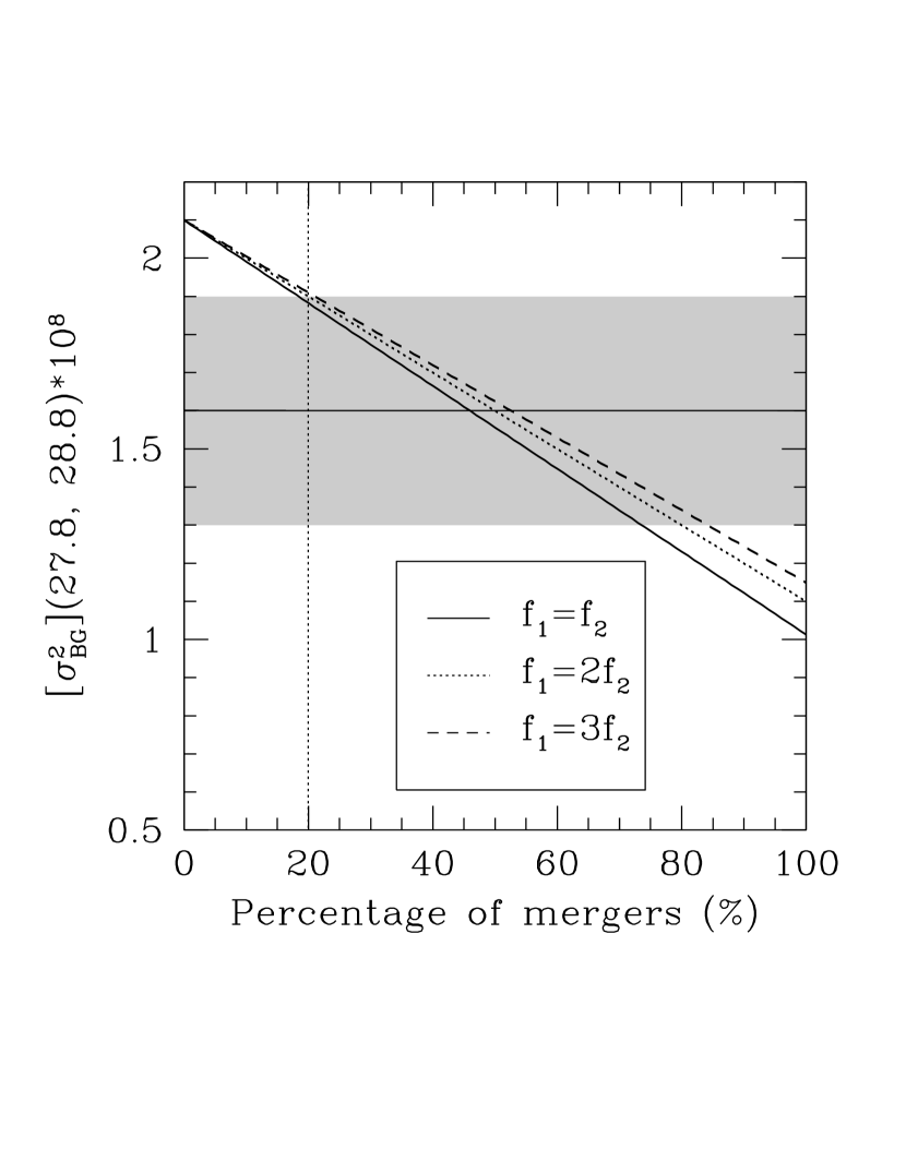
Figure 4: Effect on $[\sigma^{2}_{BG}]$ of a percentage of mergers in the Williams et al. (1996) photometric catalogue in the F606W filter. Three simple cases have been considered. i) solid line: $f_{1}=f_{2}$; ii) dashed line: $f_{1}=2f_{2}$; and iii) short-dashed line: $f_{1}=3f_{2}$, $f_{1}$ and $f_{2}$ being the fluxes of the mergered galaxies. The gray region represents the obtained $\pm 1\sigma$ SBF-measured $[\sigma^{2}_{BG}]$.

In Figure 4 we show the results of $n(m)$-estimated $[\sigma_{\rm BG}^{2}]$ for the three cases and the F606W filter, considering different values of the percentage of merged objects. It can be seen that, even in the very pessimistic case where $50\%$ of the Williams et al. (1996) objects are mergers of two identical galaxies, their influence on $[\sigma_{\rm BG}^{2}]$ is less than $25\%$. For example, in a perhaps more realistic situation in which about 20–25% of the objects are mergers of two galaxies with different magnitudes, the effect on $[\sigma_{\rm BG}^{2}]$ would smaller than $\sim$10% (see figure 4). In conclusion, the effect of mergers on $[\sigma_{\rm BG}^{2}]$ computed using the Williams et al. (1996) number counts is small and can be expected to remain below about 15% for any reasonable scenario.

We can hence proceed with our test on $[\sigma_{\rm BG}^{2}]$ for the [27.8, 28.8] interval using the Williams et al. (1996) data. The results for SBF-measured and $n(m)$-estimated $[\sigma_{\rm BG}^{2}]$ are given in Table 9. The value of $n(m)$-estimated $[\sigma_{\rm BG}^{2}]$ has been computed using Williams et al. (1996) and Metcalfe et al. (2001) data. The results are given in columns 2 and 3, while column 4 lists the $n(m)$-measured $[\sigma_{\rm BG}^{2}]$ values. It can be seen that they are not compatible with the values obtained from the Metcalfe et al. (2001) data, as expected.

On the other hand, the $n(m)$-estimated $[\sigma_{\rm BG}^{2}]$ obtained from the Williams et al. (1996) number counts and the SBF-measured $[\sigma_{\rm BG}^{2}]$ are very close. In order to compare them with more detail, let analyze figure 4 again. The $n(m)$-measured $[\sigma_{\rm BG}^{2}]$ value for the F606W filter and its error interval have also been plotted in the figure (shadowed region). It can be seen now that they fully coincide if a number of mergers about 20–30% is assumed. This situation is realistic and compatible with Metcalfe et al. (2001)’s claims.

Summarizing, the test has been successful and shows that the SBF measurements are well-calibrated.

5 Discussion

In this section, SBF-measured $\sigma_{\rm BG}^{2}$ results (listed in Table 7) and the $n(m)$-estimated $\sigma_{\rm BG}^{2}$ values obtained from both the Williams et al. (1996) and Metcalfe et al. (2001) data (listed in Table 3) will be compared. In the following, two possibilities will be considered and their consequences discussed: i) that the Williams et al. (1996) data represent the right differential number counts, and ii) that the Metcalfe et al. (2001) number counts are correct. The obtained SBF measurements will be used to test the validity of these possibilities and, as a result, a final $n(m)$ will be proposed.

5.1 Option A: Assuming Williams et al. (1996) galaxy number counts

Here we assume that the Williams et al. (1996) number counts are correct. Comparing the $n(m)$-estimated $\sigma_{\rm BG}^{2}$ obtained using Williams et al. (1996) data and SBF-measured $\sigma_{\rm BG}^{2}$, it can be seen that the former are much larger. There are only two possible sources to account for this discrepancy: first, a faint unresolved stellar population, belonging to the Milky Way halo, could be responsible of the excess in the SBF signal; and second, the faint end of $n(m)$ is different from the fitted one used here to evaluate the $n(m)$-estimated $\sigma_{\rm BG}^{2}$. In the first case, SBF results may be used to characterize such a halo population. In the second case, SBF results may be used to deduce a new faint end of $n(m)$ able to account for the SBF-measured $\sigma_{\rm BG}^{2}$.

We shall analyze both possibilities in detail and discuss the feasibility of each one and its compatibility with the observations; finally, we shall deduce its implications for $n(m)$.

5.1.1 Faint Milky Way halo stars

Here, we will consider a Milky Way halo population of faint stars be responsible of the observed excess in the SBF signal. We will firstly deduce the halo population necessary to cause this SBF signal excess. In order to check the feasibility of this hypothesis, the obtained halo population will then be compared with observations in the HDF.

Lets consider a simple population of objects with absolute magnitude $M$ following the standard spatial distribution used by Binney & Tremaine (1987):

$$\rho(r)dr=\frac{\rho_{0}}{1+(r/a)^{\alpha}}dr,$$ (14)

where $\rho(r)dr$ is the number of objects per pc³ at a distance from the Milky Way center between $r$ and $r+dr$; $a$ is the core radius, and $\rho_{0}$ is the object density in the Milky Way center. For simplicity we take $\alpha=2$.

To derive the SBF signal from the former population, we must first express the equations in terms of distance from the Sun ($\delta$). This can be done using:

$$r^{2}=\delta^{2}+r_{0}^{2}-2\delta r_{0}\cos b\cos l,$$ (15)

where $r_{0}$ is the galactocentric radius, i.e., the distance from the Sun to the Milky Way center, and $(b,l)$ are galactic coordinates. The spatial distribution of objects expressed in spherical coordinates is then:

$$n(\delta,\theta,\varphi)dV{}$$ (16)

$${}=\frac{\rho_{0}a^{2}}{a^{2}+r_{0}^{2}+\delta^{2}-2r_{0}\delta\sin\theta\cos\varphi}\delta^{2}\sin\theta d\delta d\theta d\varphi.$$

Integrating for the HDF-N and considering its coordinates $l=127\arcdeg$ and $b=54\arcdeg$, the former expression is reduced to:

$$n(\delta)d\delta\simeq\frac{1.38\times 10^{-13}\rho_{0}a^{2}\delta^{2}}{a^{2}+r_{0}^{2}+\delta^{2}-0.7075r_{0}\delta}d\delta.$$ (17)

Now, $n(\delta)d\delta$ can be written in terms of magnitudes by means of the distance modulus to obtain:

$$n(m)dm{}$$ (18)

$${}=\frac{6.36\times 10^{-11}\rho_{0}a^{2}10^{0.6(m-M)}}{a^{2}+r_{0}^{2}+100\times 10^{0.4(m-M)}+7.075r_{0}10^{0.2(m-M)}}dm.$$

The number of resolved objects with $m<28.8$ that should appear in the HDF-N, ($N_{\rm HDF-N}^{(m<28.8)}$) can be now deduced from eq. 18, as well as the variance that the faint part of the population ($m>28.8$) would produce ($\sigma_{\rm HDF-N}^{2(m>28.8)}$):

$$N_{\rm HDF-N}^{(m<28.8)}=1.31\times 10^{-4}\rho_{0}a^{2}{}$$ (19)

$${}\times\int_{-\infty}^{28.8-M}\frac{10^{0.6x}}{a^{2}+r_{0}^{2}+100\times 10^{0.4x}+7.075r_{0}10^{0.2x}}dx,$$

$$\sigma_{\rm HDF-N}^{2(m>28.8)}=6.36\times 10^{-11}\rho_{0}a^{2}10^{0.8(m_{1}^{*}-M)}{}$$ (20)

$${}\times\int_{28.8-M}^{\infty}\frac{10^{-0.2x}}{a^{2}+r_{0}^{2}+100\times 10^{0.4x}+7.075r_{0}10^{0.2x}}dx.$$

In order to compare these predictions with the HDF data, the $V_{606}$ filter results have been used. A value must be assumed for the core radius, $a$. Realistic values are around $2000$ pc (Bahcall & Soneira, 1980), but $500$ pc and $8000$ pc have been also used to check a wide interval of possibilities. Making $\sigma_{\rm HDF-N}^{2(m>28.8)}$ equal to the $\sigma_{\rm BG}^{2}$ excess observed in the filter $V_{606}$ for $m_{c}=28.8$ (that is, $4.87\times 10^{-9}$ $\left[DN/({\rm s\ pix})\right]^{2}$, see Tables 3 and 7) and introducing the value in eq. 20, the central density $\rho_{0}$ can be obtained and used in eqs  14 and 18 to derive $\rho_{\rm local}$ and $N_{\rm HDF-N}^{(m<28.8)}$. Results are plotted in Fig. 5, where $\rho_{\rm local}$ and $N_{\rm HDF-N}^{(m<28.8)}$ are shown as functions of $M_{\rm F606W}$, the absolute magnitude of the halo population objects.

This figure implies the existence of a large number of halo objects that should be present in the HDF images. Note that $N_{\rm HDF-N}^{(m<28.8)}$ is greater than $\sim$250 in all cases. This result is not compatible with the HDF-N observations, where no obvious stars are present, except for a few 20th magnitude ones, (Kawaler, 1996; Flynn, Gould, & Bahcall, 1996).

In conclusion, the observed excess in SBF-measured $\sigma_{\rm BG}^{2}$ cannot be produced by objects belonging to the Milky Way halo. Otherwise a large number of resolved objects from this halo population would show up in the HDF-N images, which is not the case.

5.1.2 Faint galaxy number counts

If the observed $\sigma_{BG}^{2}$ excess cannot be produced by Milky Way halo objects, the only possibility is that it is caused by faint galaxies. The large excess obtained in the SBF-measured $\sigma_{BG}^{2}$ with respect to the $n(m)$-estimated $\sigma_{BG}^{2}$ would imply an increase in the slope of $n(m)$ at some magnitude fainter than $m_{c}=28.8$. This slope can be computed by fitting the $n(m)$-estimated $\sigma_{BG}^{2}$ to our SBF-measured $\sigma_{BG}^{2}$ and taking the slope as a free parameter. If it is assumed that the slope change occurs at $m_{c}=28.8$ for all filters, the resulting slopes for the fainter range are $\gamma=0.60$, $0.44$, and $0.54$ for $B_{450}$, $V_{606}$, and $I_{814}$, respectively. These slopes would be valid up to $B_{450}=34.4$, $V_{606}=31.9$, and $I_{814}=32.5$ at least since the contribution of fainter magnitudes to $\sigma_{BG}^{2}$ becomes smaller than the uncertainties in the SBF-measured $\sigma_{BG}^{2}$ results. If the slope change were to occur at a magnitude fainter than 28.8, it would result in a steeper $n(m)$. In any case, such big changes in the slope of $n(m)$ seem unrealistic. In our opinion, this possibility should be rejected. As a consequence, it must be concluded that the Williams et al. (1996) data are incomplete.

5.2 Option B: Assuming Metcalfe et al. (2001) galaxy number counts

Assuming that the Metcalfe et al. (2001) differential number counts are correct, the SBF-measured $\sigma_{\rm BG}^{2}$ results listed in Table 7 and the $n(m)$-estimated $\sigma_{\rm BG}^{2}$ values obtained using the Metcalfe et al. (2001) data, listed in Table 3, can be compared.

It can be seen that the SBF-measured and $n(m)$-estimated $\sigma_{\rm BG}^{2}$ coincide within the error bars for the F814W filter, and is very similar for the F450W filter. Only in the filter F606W some differences arise. This implies that extrapolation of the Metcalfe et al. (2001) $n(m)$ function to magnitudes fainter than 28.8 accounts almost entirely for the measured SBF signal, thus indicating a high level of precision in the Metcalfe et al. (2001) data.

However, as SBF-measured and $n(m)$-estimated $\sigma_{\rm BG}^{2}$ present slight differences in the F450W and F606W filters, the most likely $n(m)$ function that completely fits our SBF measurements can be determined. This will be done in the next subsection.

5.3 The galaxy differential number counts beyond $V_{606}=28.8$

In this section, the most likely $n(m)$ function will be obtained for magnitudes fainter than 28.8. We consider that the most likely $n(m)$ function is that which fits our SBF measurements.

An $n(m)$ function is completely determined by giving the slope ($\gamma$) and the number of galaxies in a given area and magnitude interval ($n_{m}$). In particular we consider $n_{29}$, computed for the magnitude interval [28.75, 29.25] and the area of the HDF-N. Note that there are infinite sets of ($\gamma$, $n_{29}$) that can produce the same SBF signal. In Figure 6, the ($\gamma$, $n_{29}$) pairs that can account for our measured SBF signal have been plotted (solid lines) for the F450W, F606W, and F814W filters. With short-dashed lines we represent the ($\gamma$, $n_{29}$) pairs that would produce the SBF measurements $\pm 1\sigma$. In this figure, the ($\gamma$, $n_{29}$) sets corresponding to the extrapolation of $n(m)$ obtained from Williams et al. (1996) (solid circle) and Metcalfe et al. (2001) data (open circle) have also been plotted.

It can be seen in Figure 6 that the Metcalfe et al. (2001) ($\gamma$, $n_{29}$) reproduce our SBF results for the F814W filter, as previously shown. For F450W, the Metcalfe et al. (2001) ($\gamma$, $n_{29}$) is very close to our SBF measurements. In all cases (except for F606W), the Williams et al. (1996) ($\gamma$, $n_{29}$) results are far from our SBF results, as previously argued.

The most likely $n(m)$ function can be obtained from Figure 6. We assume that, for each filter, the best $n(m)$ estimate for magnitudes fainter than 28.8 is given by the nearest point of the solid lines to the Metcalfe et al. (2001) point. In this case, results for the slopes are $\gamma=0.27$, $0.21$, and $0.26$ for $B_{450}$, $V_{606}$, and $I_{814}$, respectively.

The results are listed in Table 10 and plotted in Figure 7 (solid lines). The slopes obtained are valid down to magnitude $31$ at least. The contribution to the SBF signal by objects of fainter magnitudes is less than the uncertainty in the SBF measurements. This value represents an extension of more than two magnitudes beyond the limits of the previous photometric studies by Williams et al. (1996) and Metcalfe et al. (2001). It should also be mentioned that, within the uncertainties and except for the objects that could be merged into brighter ones in Metcalfe et al. (2001), it is free from incompleteness.

6 Conclusions

In this paper, the faint end of the differential galaxy number counts, $n(m)$, has been studied by means of SBF measurements. Once the contribution from cosmic rays has been evaluated and eliminated from the SBF signal, the background PSF-convolved variance originating from faint objects has been carefully analyzed. Our conclusions can be summarized as follows:

• Comparing the SBF-measured $\sigma_{\rm BG}^{2}$ with the $n(m)$-estimated $\sigma_{\rm BG}^{2}$ predicted by the extrapolation of Williams et al. (1996) number counts a clear excess has been found in the measured signal. The possibility that the excess might be produced by Milky Way halo stars is ruled out because it would be totally incompatible with the resolved stellar population present in the HDF. On the other hand, if this excess is caused by a faint galaxy population modifying the faint end of $n(m)$, then the required slopes for magnitudes fainter than 28.8 are $\gamma=0.60$, $0.44$, and $0.54$ for $B_{450}$, $V_{606}$, and $I_{814}$, respectively. Such big changes in the $n(m)$ slope seem unrealistic. In our opinion, this possibility should be rejected. In conclusion, the Williams et al. (1996) number counts are not compatible with our SBF measurements, probably owing to the incompleteness in their data.

• Comparing the SBF-measured $\sigma_{\rm BG}^{2}$ with the $n(m)$-estimated $\sigma_{\rm BG}^{2}$, predicted by the extrapolation of Metcalfe et al. (2001) number counts, we find that they coincide within the error bars for the F814W and F450W filters and are similar for F606W. This implies that the extrapolation of the Metcalfe et al. (2001) $n(m)$ function to magnitudes fainter than 28.8 nearly accounts for the measured SBF signal, indicating a high level of precision in the Metcalfe et al. (2001) results.

• The most likely $n(m)$ function has been obtained fitting our SBF results. Results for the $n(m)$ slope for magnitudes fainter than $28.8$ are $\gamma=0.27$, $0.21$, and $0.26$ for $B_{450}$, $V_{606}$, and $I_{814}$, respectively. The obtained slopes are valid down to magnitude $31$ at least. This value represents an extension of more than two magnitudes beyond the limits of the previous photometric studies by Williams et al. (1996) and Metcalfe et al. (2001).

Figure 1: Differential number counts of the detected sources by Williams et al. (1996) (filled circles) and Metcalfe et al. (2001) (open circles) in the F450W, F606W and F814W filters. Solid lines represents the fitted $n(m)$ functions. It can be clearly seen the slope change around magnitude 26 found by Williams et al. (1996).

Figure 2: Example of a SBF measurement: results for the average image in the F450W filter with $m_{c}=28.8$. Solid line represents the power spectrum fitting. The observed discrepancy at low wave numbers between the obtained power spectrum and the fit is due to large scale fluctuations in the background brightness of the images. The power-spectrum fitting procedure is the following: eq. 2 is used to fit the power spectrum for wave numbers in the range [$k_{0}$, $k_{\rm max}$], $k_{\rm max}$ being the highest wave number of the computed power spectrum, and $k_{0}$ a number which we vary from 0 to $k_{\rm max}$. As a result, two functions, $P_{0}(k_{0})$ and $P_{1}(k_{0})$, are obtained. The function $P_{0}(k_{0})$ is also shown (small boxes). It can be seen that this function exhibits a “plateau” region. The final adopted result and its uncertainty for $P_{0}$ are obtained computing the average and standard deviation of $P_{0}(k_{0})$ in the plateau interval. For the $P_{1}$ measurement, the procedure is exactly the same as for $P_{0}$.

Figure 3: $P_{0}$ results versus the sky level in WF2 F606W images with $m_{c}=27.8$. The absence of a trend indicates that flat-fielding errors are not significant in the measurement of $P_{0}$.

Figure 5: Local density ($\rho_{\rm local}$) and number of objects in the HDF-N images up to magnitude $V_{606}=28.8$ ($N_{\rm HDF-N}(28.8)$) predicted by the considered halo model for three possible values of core radius, $a$. These results have been obtained assuming that the excess in $P_{0}$ is completely produced by halo objects. It can be seen that the model predictions are not compatible with observations. This implies that the observed $P_{0}$ excess cannot be caused by halo objects. See text for details.

Figure 6: The $n(m)$ slope, $\gamma$, versus the number of galaxies in the HDF-N in the magnitude interval [28.75, 29.25], $n_{29}$, for the F450W, F606W, and F814W filters. Solid lines: the pairs ($\gamma$, $n_{29}$) that would produce our measured SBF signal; short-dashed lines: the pairs ($\gamma$, $n_{29}$) that would produce the SBF measurements $\pm 1\sigma$; filled circle: the set ($\gamma$, $n_{29}$) corresponding to the extrapolation of $n(m)$ obtained from the Williams et al. (1996) data; open circle: the same corresponding to Metcalfe et al. (2001). It can be seen that the Metcalfe et al. (2001) number counts nearly fit out SBF measurements. See text for details.

Figure 7: $n(m)$ final results in the F450W, F606W and F814W filters. Filled circles represent Williams et al. (1996) differential number counts, open circles are the results from Metcalfe et al. (2001). Solid line represents the obtained faint end (fainter than magnitude 28.8) of $n(m)$. The obtained $n(m)$ function is valid down to magnitude 31, at least.

Table 1: The data.

Image	Filter	$t_{\rm exp}(s)$
F450W.d1.dark	F450W	17200
F450W.d2.dark	F450W	7900
F450W.d3.dark	F450W	11500
F450W.d4.dark	F450W	12400
F450W.d5.dark	F450W	11800
F450W.d6.dark	F450W	12900
F450W.d8.dark	F450W	13100
F450W.d9.dark	F450W	10700
F606W.d1.dark	F606W	6700
F606W.d2.dark	F606W	4800
F606W.d3.dark	F606W	6450
F606W.d4.dark	F606W	10300
F606W.d5.dark	F606W	15600
F606W.d6.dark	F606W	17300
F606W.d7.dark	F606W	14600
F606W.d8.dark	F606W	10100
F606W.d9.dark	F606W	7100
F606W.d10.dark	F606W	8300
F606W.d11.dark	F606W	7800
F814W.d1.dark	F814W	10800
F814W.d2.dark	F814W	12200
F814W.d3.dark	F814W	14200
F814W.d4.dark	F814W	12000
F814W.d5.dark	F814W	13000
F814W.d6.dark	F814W	13100
F814W.d8.dark	F814W	5800
F814W.d9.dark	F814W	12900

Table 2: HDF photometric zero points.

Filter	Chip	Magnitude ($AB$ system)
F450W	PC1	21.92
F450W	WF2	21.93
F450W	WF3	21.93
F450W	WF4	21.90
F606W	PC1	23.02
F606W	WF2	23.02
F606W	WF3	23.03
F606W	WF4	23.00
F814W	PC1	22.08
F814W	WF2	22.09
F814W	WF3	22.09
F814W	WF4	22.07

Table 3: $n(m)$-estimated $\sigma_{\rm BG}^{2}$, in units of $[\frac{DN}{\rm s\times pix}]^{2}$

$m_{\rm c}$	F450W	F606W	F814W
From Williams et al. (1996) data
27.8	2.82 $\times 10^{-9}$	2.74 $\times 10^{-8}$	5.50 $\times 10^{-9}$
28.8	6.45 $\times 10^{-10}$	6.43 $\times 10^{-9}$	1.32 $\times 10^{-9}$
From Metcalfe et al. (2001) data
27.8	7.20 $\times 10^{-9}$	5.76 $\times 10^{-8}$	1.05 $\times 10^{-8}$
28.8	2.23 $\times 10^{-9}$	1.62 $\times 10^{-8}$	3.04 $\times 10^{-9}$

Table 4: F450W average image ($m_{\rm c}=27.8$) SBF results varying the patch radius, in units of $10^{-9}\times[\frac{DN}{\rm s\times pix}]^{2}$

Radius (pixels)	$P_{0}$	$P_{1}$
15 (adopted)	4.52$\pm$0.06	9.01$\pm$0.02
20	4.45$\pm$0.05	9.05$\pm$0.02
25	4.50$\pm$0.06	9.03$\pm$0.02
30	4.47$\pm$0.06	9.00$\pm$0.02

Table 5: SBF results for $m_{\rm c}=27.8$, in units of $10^{-8}\times[\frac{DN}{\rm s\times pix}]^{2}$

Image	PC1		WF2		WF3		WF4
	$P_{0}$	$P_{1}$	$P_{0}$	$P_{1}$	$P_{0}$	$P_{1}$	$P_{0}$	$P_{1}$
F450W.d1.dark	1.90 $\pm$ 0.16	3.86 $\pm$ 0.01	1.05 $\pm$ 0.11	5.4 $\pm$ 0.1	0.86 $\pm$ 0.05	5.4 $\pm$ 0.1	1.09 $\pm$ 0.05	4.6 $\pm$ 0.1
F450W.d2.dark	3.04 $\pm$ 0.10	7.21 $\pm$ 0.01	1.89 $\pm$ 0.07	11.4 $\pm$ 0.1	1.70 $\pm$ 0.23	10.8$\pm$ 0.1	1.13 $\pm$ 0.17	10.0 $\pm$ 0.1
F450W.d3.dark	1.48 $\pm$ 0.06	5.25 $\pm$ 0.01	1.06 $\pm$ 0.10	8.0 $\pm$ 0.1	1.01 $\pm$ 0.07	7.8 $\pm$ 0.1	1.33 $\pm$ 0.10	6.9 $\pm$ 0.1
F450W.d4.dark	1.39 $\pm$ 0.09	4.45 $\pm$ 0.01	1.34 $\pm$ 0.06	6.9 $\pm$ 0.1	1.25 $\pm$ 0.09	6.7 $\pm$ 0.1	1.42 $\pm$ 0.13	6.2 $\pm$ 0.1
F450W.d5.dark	1.73 $\pm$ 0.09	5.18 $\pm$ 0.01	1.21 $\pm$ 0.05	7.5 $\pm$ 0.1	1.36 $\pm$ 0.04	7.2 $\pm$ 0.1	1.89 $\pm$ 0.07	6.3 $\pm$ 0.1
F450W.d6.dark	1.47 $\pm$ 0.06	4.31 $\pm$ 0.01	1.04 $\pm$ 0.12	6.9 $\pm$ 0.1	1.22 $\pm$ 0.03	6.7 $\pm$ 0.1	1.00 $\pm$ 0.08	6.1 $\pm$ 0.1
F450W.d8.dark	1.24 $\pm$ 0.05	4.32 $\pm$ 0.01	0.77 $\pm$ 0.08	6.9 $\pm$ 0.1	1.40 $\pm$ 0.05	6.7 $\pm$ 0.1	0.76 $\pm$ 0.11	6.1 $\pm$ 0.1
F450W.d9.dark	2.10 $\pm$ 0.08	5.95 $\pm$ 0.01	1.13 $\pm$ 0.11	8.9 $\pm$ 0.1	0.98 $\pm$ 0.21	8.5 $\pm$ 0.1	1.70 $\pm$ 0.06	7.7 $\pm$ 0.1
Average image	0.29 $\pm$ 0.03	0.636 $\pm$ 0.001	0.452$\pm$ 0.006	0.901$\pm$ 0.002	0.563 $\pm$ 0.014	0.847$\pm$ 0.004	0.441 $\pm$ 0.006	0.762 $\pm$ 0.002
F606W.d1.dark	4.50 $\pm$ 0.24	17.6 $\pm$ 0.1	7.7 $\pm$ 0.3	36.8 $\pm$ 0.1	6.8 $\pm$ 0.9	37.4 $\pm$ 0.2	2.5 $\pm$ 0.2	35.2 $\pm$ 0.1
F606W.d2.dark	6.1 $\pm$ 0.5	27.2 $\pm$ 0.1	8.2 $\pm$ 0.2	54.9 $\pm$ 0.4	5.5 $\pm$ 0.6	56.5 $\pm$ 0.1	1.4 $\pm$ 0.9	52.5 $\pm$ 0.3
F606W.d3.dark	4.7 $\pm$ 0.6	22.2 $\pm$ 0.1	5.5 $\pm$ 0.5	42.7 $\pm$ 0.2	6.2 $\pm$ 1.7	42.1 $\pm$ 0.3	8.8 $\pm$ 0.6	42.6 $\pm$ 0.3
F606W.d4.dark	2.92 $\pm$ 0.21	13.3 $\pm$ 0.1	4.2 $\pm$ 0.4	26.1 $\pm$ 0.1	6.2 $\pm$ 0.5	25.7 $\pm$ 0.1	5.2 $\pm$ 0.4	23.9 $\pm$ 0.1
F606W.d5.dark	4.71 $\pm$ 0.18	9.3 $\pm$ 0.1	6.1 $\pm$ 0.2	17.6 $\pm$ 0.1	6.8 $\pm$ 0.6	19.1 $\pm$ 0.2	4.5 $\pm$ 0.6	16.8 $\pm$ 0.2
F606W.d6.dark	2.48 $\pm$ 0.09	7.5 $\pm$ 0.1	6.5 $\pm$ 0.3	16.2 $\pm$ 0.1	6.0 $\pm$ 0.2	17.4 $\pm$ 0.1	5.2 $\pm$ 0.4	14.8 $\pm$ 0.1
F606W.d7.dark	3.52 $\pm$ 0.16	9.0 $\pm$ 0.1	6.3 $\pm$ 0.3	18.2 $\pm$ 0.1	7.1 $\pm$ 0.4	18.6 $\pm$ 0.1	4.3 $\pm$ 0.2	16.7 $\pm$ 0.1
F606W.d8.dark	3.6 $\pm$ 0.4	12.6 $\pm$ 0.1	7.4 $\pm$ 0.5	25.2 $\pm$ 0.1	6.7 $\pm$ 0.6	25.7 $\pm$ 0.1	5.6 $\pm$ 0.4	24.2 $\pm$ 0.2
F606W.d9.dark	5.17 $\pm$ 0.24	20.3 $\pm$ 0.1	6.6 $\pm$ 0.4	37.6 $\pm$ 0.1	7.8 $\pm$ 0.3	38.4 $\pm$ 0.2	6.5 $\pm$ 0.4	33.7 $\pm$ 0.2
F606W.d10.dark	4.50 $\pm$ 0.13	15.1 $\pm$ 0.1	7.3 $\pm$ 0.4	30.2 $\pm$ 0.1	7.6 $\pm$ 0.6	31.3 $\pm$ 0.2	4.7 $\pm$ 0.7	28.2 $\pm$ 0.2
F606W.d11.dark	5.37 $\pm$ 0.16	15.5 $\pm$ 0.1	5.5 $\pm$ 0.8	31.3 $\pm$ 0.2	7.4 $\pm$ 0.8	32.3 $\pm$ 0.2	4.4 $\pm$ 0.7	28.9 $\pm$ 0.2
Average image	0.96 $\pm$ 0.18	1.38 $\pm$ 0.01	3.19 $\pm$ 0.13	2.68 $\pm$ 0.02	3.08 $\pm$ 0.20	2.52 $\pm$ 0.04	3.2 $\pm$ 0.5	1.95 $\pm$ 0.14
F814W.d1.dark	2.24 $\pm$ 0.10	7.94 $\pm$ 0.01	0.83 $\pm$ 0.16	14.9 $\pm$ 0.1	1.5 $\pm$ 0.3	15.7 $\pm$ 0.1	1.8 $\pm$ 0.3	14.7 $\pm$ 0.1
F814W.d2.dark	1.89 $\pm$ 0.11	7.59 $\pm$ 0.01	1.99 $\pm$ 0.15	13.3 $\pm$ 0.1	3.23 $\pm$ 0.09	24.4 $\pm$ 0.1	1.70 $\pm$ 0.18	13.3 $\pm$ 0.1
F814W.d3.dark	2.04 $\pm$ 0.04	6.13 $\pm$ 0.01	1.34 $\pm$ 0.17	11.8 $\pm$ 0.1	1.68 $\pm$ 0.11	11.9 $\pm$ 0.1	1.56 $\pm$ 0.07	10.5 $\pm$ 0.1
F814W.d4.dark	2.03 $\pm$ 0.05	6.92 $\pm$ 0.01	2.51 $\pm$ 0.23	13.0 $\pm$ 0.1	1.94 $\pm$ 0.20	13.8 $\pm$ 0.1	0.75 $\pm$ 0.10	13.6 $\pm$ 0.1
F814W.d5.dark	2.1 $\pm$ 0.3	7.00 $\pm$ 0.01	2.6 $\pm$ 0.3	12.9 $\pm$ 0.1	0.92 $\pm$ 0.14	14.6 $\pm$ 0.1	2.07 $\pm$ 0.09	13.0 $\pm$ 0.1
F814W.d6.dark	2.04 $\pm$ 0.11	6.62 $\pm$ 0.01	2.7 $\pm$ 0.3	12.1 $\pm$ 0.1	3.09 $\pm$ 0.17	13.6 $\pm$ 0.1	1.29 $\pm$ 0.16	12.8 $\pm$ 0.1
F814W.d8.dark	5.98 $\pm$ 0.14	20.26 $\pm$ 0.01	4.1 $\pm$ 0.3	27.5 $\pm$ 0.1	3.5 $\pm$ 0.3	28.6 $\pm$ 0.1	3.0 $\pm$ 0.6	25.3 $\pm$ 0.1
F814W.d9.dark	2.55 $\pm$ 0.19	6.77 $\pm$ 0.01	2.0 $\pm$ 0.4	12.6 $\pm$ 0.1	2.3 $\pm$ 0.3	13.0 $\pm$ 0.1	2.60 $\pm$ 0.07	12.0 $\pm$ 0.1
0 Average image	0.413 $\pm$ 0.019	1.074 $\pm$ 0.002	1.011 $\pm$ 0.024	1.669 $\pm$ 0.007	0.47 $\pm$ 0.05	2.057 $\pm$ 0.012	0.88 $\pm$ 0.03	1.592$\pm$ 0.011

Table 6: SBF results for $m_{\rm c}=28.8$, in units of $10^{-8}\times[\frac{DN}{\rm s\times pix}]^{2}$

Image	PC1		WF2		WF3		WF4
	$P_{0}$	$P_{1}$	$P_{0}$	$P_{1}$	$P_{0}$	$P_{1}$	$P_{0}$	$P_{1}$
F450W.d1.dark	1.53 $\pm$ 0.04	3.66 $\pm$ 0.01	0.75 $\pm$ 0.08	5.4 $\pm$ 0.1	0.62 $\pm$ 0.06	5.4 $\pm$ 0.1	0.83 $\pm$ 0.04	4.7 $\pm$ 0.1
F450W.d2.dark	3.00 $\pm$ 0.09	7.14 $\pm$ 0.01	2.01 $\pm$ 0.06	11.2 $\pm$ 0.1	1.48 $\pm$ 0.23	10.8 $\pm$ 0.1	1.46 $\pm$ 0.17	9.9 $\pm$ 0.1
F450W.d3.dark	1.43 $\pm$ 0.04	5.24 $\pm$ 0.01	1.04 $\pm$ 0.11	8.0 $\pm$ 0.1	0.81 $\pm$ 0.07	7.8 $\pm$ 0.1	1.22 $\pm$ 0.05	6.9 $\pm$ 0.1
F450W.d4.dark	1.30 $\pm$ 0.06	4.45 $\pm$ 0.01	1.09 $\pm$ 0.06	6.9 $\pm$ 0.1	1.14 $\pm$ 0.05	6.7 $\pm$ 0.1	1.23 $\pm$ 0.10	6.1 $\pm$ 0.1
F450W.d5.dark	1.68 $\pm$ 0.08	5.09 $\pm$ 0.01	0.76 $\pm$ 0.06	7.6 $\pm$ 0.1	1.2 $\pm$ 0.3	7.2 $\pm$ 0.1	1.49 $\pm$ 0.04	6.4 $\pm$ 0.1
F450W.d6.dark	1.46 $\pm$ 0.05	4.31 $\pm$ 0.01	0.59 $\pm$ 0.04	6.9 $\pm$ 0.1	0.67 $\pm$ 0.18	6.8 $\pm$ 0.1	0.77 $\pm$ 0.06	6.1 $\pm$ 0.1
F450W.d8.dark	1.55 $\pm$ 0.04	4.29 $\pm$ 0.01	0.71 $\pm$ 0.07	6.9 $\pm$ 0.1	1.16 $\pm$ 0.07	6.8 $\pm$ 0.1	0.81 $\pm$ 0.07	6.0 $\pm$ 0.1
F450W.d9.dark	1.97 $\pm$ 0.06	5.96 $\pm$ 0.01	1.32 $\pm$ 0.03	8.8 $\pm$ 0.1	1.2 $\pm$ 0.4	8.4 $\pm$ 0.1	1.57 $\pm$ 0.05	7.7 $\pm$ 0.1
Average image	0.265 $\pm$ 0.009	0.626 $\pm$ 0.001	0.317$\pm$ 0.009	0.929 $\pm$ 0.003	0.341$\pm$ 0.015	0.896$\pm$ 0.004	0.247 $\pm$ 0.011	0.822 $\pm$ 0.004
F606W.d1.dark	4.75 $\pm$ 0.17	17.7 $\pm$ 0.1	5.8 $\pm$ 0.3	37.2 $\pm$ 0.1	6.0 $\pm$ 0.6	37.7 $\pm$ 0.2	2.4 $\pm$ 0.7	35.0 $\pm$ 0.3
F606W.d2.dark	5.9 $\pm$ 0.8	27.3 $\pm$ 0.1	8.9 $\pm$ 0.8	55.2 $\pm$ 0.3	4.2 $\pm$ 0.7	56.8 $\pm$ 0.2	3.6 $\pm$ 0.7	51.9 $\pm$ 0.3
F606W.d3.dark	4.9 $\pm$ 0.4	21.2 $\pm$ 0.1	3.8 $\pm$ 0.4	43.0 $\pm$ 0.1	4.7 $\pm$ 1.7	42.5 $\pm$ 0.5	6.0 $\pm$ 0.8	44.8 $\pm$ 0.3
F606W.d4.dark	2.49 $\pm$ 0.22	13.4 $\pm$ 0.1	1.9 $\pm$ 0.4	26.5 $\pm$ 0.1	4.4 $\pm$ 0.5	26.1 $\pm$ 0.2	4.2 $\pm$ 0.4	24.2 $\pm$ 0.1
F606W.d5.dark	4.69 $\pm$ 0.17	9.3 $\pm$ 0.1	4.0 $\pm$ 0.2	18.0 $\pm$ 0.1	4.4 $\pm$ 0.3	19.1 $\pm$ 0.1	3.2 $\pm$ 0.4	16.9 $\pm$ 0.2
F606W.d6.dark	2.41 $\pm$ 0.12	7.6 $\pm$ 0.1	4.2 $\pm$ 0.2	16.6 $\pm$ 0.1	4.1 $\pm$ 0.2	17.6 $\pm$ 0.4	3.8 $\pm$ 0.4	15.1 $\pm$ 0.2
F606W.d7.dark	2.9 $\pm$ 0.4	9.1 $\pm$ 0.1	4.4 $\pm$ 0.3	18.6 $\pm$ 0.1	4.5 $\pm$ 0.3	19.2 $\pm$ 0.1	3.8 $\pm$ 0.7	16.8 $\pm$ 0.3
F606W.d8.dark	3.48 $\pm$ 0.16	12.6 $\pm$ 0.1	4.9 $\pm$ 0.5	25.8 $\pm$ 0.2	5.5 $\pm$ 1.0	26.1 $\pm$ 0.3	2.5 $\pm$ 1.3	24.3 $\pm$ 0.4
F606W.d9.dark	5.3 $\pm$ 0.3	20.6 $\pm$ 0.1	4.9 $\pm$ 0.6	37.6 $\pm$ 0.2	4.4 $\pm$ 0.4	39.2 $\pm$ 0.1	4.8 $\pm$ 0.4	34.1 $\pm$ 0.2
F606W.d10.dark	4.41 $\pm$ 0.20	15.0 $\pm$ 0.1	6.2 $\pm$ 0.3	30.5 $\pm$ 0.1	6.4 $\pm$ 0.8	31.7 $\pm$ 0.2	2.6 $\pm$ 0.7	28.7 $\pm$ 0.3
F606W.d11.dark	5.6 $\pm$ 0.4	15.4 $\pm$ 0.1	3.4 $\pm$ 1.0	31.8 $\pm$ 0.3	5.3 $\pm$ 0.4	33.1 $\pm$ 0.1	2.3 $\pm$ 0.5	29.2 $\pm$ 0.2
Average image	0.557$\pm$ 0.021	1.41 $\pm$ 0.01	1.38 $\pm$ 0.15	2.81 $\pm$ 0.02	1.72 $\pm$ 0.10	2.71 $\pm$ 0.02	1.4 $\pm$ 0.3	2.43 $\pm$ 0.09
F814W.d1.dark	2.34 $\pm$ 0.08	7.99 $\pm$ 0.01	0.28 $\pm$ 0.12	15.1 $\pm$ 0.1	1.3 $\pm$ 0.3	15.9 $\pm$ 0.1	2.02 $\pm$ 0.23	14.8 $\pm$ 0.1
F814W.d2.dark	1.51 $\pm$ 0.09	7.64 $\pm$ 0.01	1.26 $\pm$ 0.13	13.3 $\pm$ 0.1	3.6 $\pm$ 0.5	26.2 $\pm$ 0.1	2.09 $\pm$ 0.17	13.2 $\pm$ 0.1
F814W.d3.dark	2.04 $\pm$ 0.04	6.10 $\pm$ 0.01	1.43 $\pm$ 0.09	11.9 $\pm$ 0.1	1.54 $\pm$ 0.22	12.0 $\pm$ 0.1	1.00 $\pm$ 0.09	10.6 $\pm$ 0.1
F814W.d4.dark	2.14 $\pm$ 0.05	6.91 $\pm$ 0.01	1.48 $\pm$ 0.08	13.3 $\pm$ 0.1	1.54 $\pm$ 0.11	13.9 $\pm$ 0.1	0.9 $\pm$ 0.4	13.9 $\pm$ 0.1
F814W.d5.dark	2.1 $\pm$ 0.3	7.02 $\pm$ 0.01	1.4 $\pm$ 0.5	13.1 $\pm$ 0.1	1.37 $\pm$ 0.16	14.9 $\pm$ 0.1	1.6 $\pm$ 0.3	13.2 $\pm$ 0.1
F814W.d6.dark	1.79 $\pm$ 0.06	6.67 $\pm$ 0.01	2.12 $\pm$ 0.12	12.5 $\pm$ 0.1	2.83 $\pm$ 0.15	13.2 $\pm$ 0.1	1.95 $\pm$ 0.12	12.9 $\pm$ 0.1
F814W.d8.dark	5.2 $\pm$ 0.5	20.81 $\pm$ 0.01	4.27 $\pm$ 0.15	27.7 $\pm$ 0.1	3.2 $\pm$ 0.3	28.6 $\pm$ 0.1	2.3 $\pm$ 0.3	25.4 $\pm$ 0.1
F814W.d9.dark	2.61 $\pm$ 0.18	6.78 $\pm$ 0.01	2.13 $\pm$ 0.12	12.3 $\pm$ 0.1	2.50 $\pm$ 0.06	13.0 $\pm$ 0.1	2.04 $\pm$ 0.07	12.3 $\pm$ 0.1
Average image	0.397 $\pm$ 0.022	1.084 $\pm$ 0.002	0.54 $\pm$ 0.03	1.787 $\pm$ 0.007	0.484$\pm$0.022	2.140 $\pm$0.006	0.43 $\pm$ 0.03	1.763$\pm$ 0.010

Table 7: SBF-measured $\sigma_{\rm BG}^{2}$ and $\sigma_{\rm CR}^{2}$ results, in units of $10^{-8}\times[\frac{DN}{\rm s\times pix}]^{2}$

	F450W		F606W		F814W
Chip	$\sigma_{\rm BG}^{2}$	$\sigma_{\rm cr}^{2}$	$\sigma_{\rm BG}^{2}$	$\sigma_{\rm cr}^{2}$	$\sigma_{\rm BG}^{2}$	$\sigma_{\rm cr}^{2}$
$m_{\rm c}=27.8$
PC1	0.35 $\pm$ 0.16	0.215 $\pm$ 0.007	3.1 $\pm$ 0.9	0.336 $\pm$ 0.020	0.48 $\pm$ 0.10	0.314 $\pm$ 0.006
WF2	0.347 $\pm$ 0.008	0.105 $\pm$ 0.005	2.26 $\pm$ 0.13	0.331 $\pm$ 0.018	0.83 $\pm$ 0.03	0.176 $\pm$ 0.012
WF3	0.468 $\pm$ 0.015	0.094 $\pm$ 0.006	2.72 $\pm$ 0.20	0.36 $\pm$ 0.03	0.52 $\pm$ 0.05	0.218 $\pm$ 0.013
WF4	0.320 $\pm$ 0.008	0.121 $\pm$ 0.005	3.0 $\pm$ 0.5	0.16 $\pm$ 0.05	0.74 $\pm$ 0.04	0.139 $\pm$ 0.021
SBF-measured $\sigma_{\rm BG}^{2}$	0.37 $\pm$ 0.04		2.8 $\pm$ 0.3		0.64 $\pm$ 0.03
$m_{\rm c}=28.8$
PC1	0.26 $\pm$ 0.05	0.211 $\pm$ 0.006	0.91 $\pm$ 0.11	0.370 $\pm$ 0.011	0.42 $\pm$ 0.12	0.297 $\pm$ 0.012
WF2	0.214 $\pm$ 0.010	0.102 $\pm$ 0.004	1.04 $\pm$ 0.15	0.342 $\pm$ 0.021	0.36 $\pm$ 0.03	0.179 $\pm$ 0.011
WF3	0.242 $\pm$ 0.019	0.099 $\pm$ 0.011	1.40 $\pm$ 0.10	0.32 $\pm$ 0.03	0.23 $\pm$ 0.03	0.251 $\pm$ 0.013
WF4	0.115 $\pm$ 0.012	0.132 $\pm$ 0.004	1.2 $\pm$ 0.3	0.22 $\pm$ 0.04	0.24 $\pm$ 0.03	0.187 $\pm$ 0.013
SBF-measured $\sigma_{\rm BG}^{2}$	0.208 $\pm$ 0.014		1.13 $\pm$ 0.09		0.31 $\pm$ 0.03

Table 8: Computed and observed $P_{1}$ for F450W (WF2) and $m_{\rm c}=28.8$, in units of $10^{-8}\times[\frac{DN}{\rm s\times pix}]^{2}$

Image	Computed $P_{1}$	Observed $P_{1}$
F450W.d1.dark	5.2	5.48 $\pm$ 0.02
F450W.d2.dark	11.5	11.25 $\pm$ 0.01
F450W.d3.dark	7.8	8.02 $\pm$ 0.03
F450W.d4.dark	6.9	6.96 $\pm$ 0.02
F450W.d5.dark	7.3	7.62 $\pm$ 0.02
F450W.d6.dark	6.7	6.99 $\pm$ 0.01
F450W.d8.dark	6.6	6.91 $\pm$ 0.02
F450W.d9.dark	8.3	8.81 $\pm$ 0.01

Table 9: $n(m)$-estimated and SBF-measured $[\sigma_{\rm BG}^{2}]$, in units of $10^{-8}\times[\frac{DN}{\rm s\times pix}]^{2}$

Filter	$n(m)$-estimated	$n(m)$-estimated	SBF-measured
	using Williams et al. (1996)	using Metcalfe et al. (2001)
F450W	0.22	0.50	0.16 $\pm$ 0.04
F606W	2.10	4.14	1.6 $\pm$ 0.3
F814W	0.42	0.75	0.33 $\pm$ 0.04

Table 10: $n(m)$ Results

Filter	$\gamma$	SBF limiting magnitude
F450W	0.27	31.0
F606W	0.21	30.7
F814W	0.26	30.8

References

- Bahcall & Soneira (1980) Bahcall, J. N., & Soneira, R. M. 1980, ApJS, 44, 73
- Binney & Tremaine (1987) Binney, J., & Tremaine, S. 1987, Galactic Dynamics (Princeton: Princeton University Press)
- Blakeslee (1999) Blakeslee, J. P. 1999, AJ, 118, 1506
- Blakeslee & Tonry (1995) Blakeslee, J. P., & Tonry, J. L. 1995, ApJ, 442, 579
- Blakeslee, Vazdekis, & Ajhar (2001) Blakeslee, J. P., Vazdekis, A., & Ajhar, E. A. 2001, MNRAS, 320, 193
- Ellis (1997) Ellis, R. S. 1997, ARA&A, 35, 389
- Ferguson (1998) Ferguson, H. C. 1998. In The Hubble Deep Field, ed. M. Livio, S. M. Fall, & P. Madau (Cambridge: Cambridge University Press), 181
- Ferguson, Dickinson, & Williams (2000) Ferguson, H. C., Dickinson, M., & Williams, R. 2000, ARA&A, 38, 667
- Flynn, Gould, & Bahcall (1996) Flynn, C., Gould, A., & Bahcall, J. N. 1996, ApJ, 466, L55
- Hidalgo, Marín-Franch, & Aparicio (2003) Hidalgo, S., Marín-Franch, A., & Aparicio, A. 2003, AJ, 125, 1247
- Jensen et al. (1998) Jensen, J. B., Tonry, J. L., & Luppino, G. A. 1998, ApJ, 505, 111
- Kawaler (1996) Kawaler, D. K. 1996, ApJ, 467, L61
- Koo & Kron (1988) Koo, D. C., & Kron, R. G. 1988, ARA&A, 30, 613
- Lanzzetta, Yahil, & Fernández-Soto (1996) Lanzzetta, K. M., Yahil, A., & Fernández-Soto, A. 1996, Nature, 381, 759
- Liu, Charlot, & Graham (2000) Liu, M. C., Charlot, S., & Graham, J. R. 2000, ApJ, 543, 644
- Marín-Franch & Aparicio (2002) Marín-Franch, A., & Aparicio, A. 2002, ApJ, 568, 174
- Marín-Franch & Aparicio (2003) Marín-Franch, A., & Aparicio, A. 2003, ApJ, 585, 714
- Metcalfe et al. (1996) Metcalfe, N,. Shanks, T., Campos, A., Fong, R., & Gardner, J. P. 1996, Nature, 383, 236
- Metcalfe et al. (2001) Metcalfe, N., Shanks, T., Campos, A., McCracken, H. J., & Fong, R. 2001, MNRAS, 323, 795
- Oke (1974) Oke, J. B. 1974, ApJS, 27, 21
- Pozzetti et al. (1998) Pozzetti, L., Madau, P., Zamorani, G., Ferguson, H. C., & Bruzual, G. 1998, MNRAS, 298, 1133
- Sandage (1988) Sandage, A. 1988, ARA&A, 26, 561
- Tonry et al. (2000) Tonry, J. L., Blakeslee, J. P., Ajhar, E. A., & Dressler, A, 2000, ApJ, 530, 625
- Tonry et al. (2001) Tonry, J. L., Dressler, A., Blakeslee, J. P., Ajhar, E. A., Fletcher, A. B., Luppino, G. A., Metzger, M. R., & Moore, C. B. 2001, ApJ, 546, 681
- Tonry & Schneider (1988) Tonry, J. L., & Schneider, D. P. 1988, AJ, 96, 807
- Williams et al. (1996) Williams, R. E., et al. 1996, AJ, 112, 1335