The Probability Distribution Function of Light in the Universe: Results from Hydrodynamic Simulations
Abstract
While second and higher order correlations of the light distribution have received extensive study, the lowest order probability distribution function (PDF) — the probability that a unit volume of space will emit a given amount of light — has received very little attention. We estimate this function with the aid of hydrodynamic simulations of the CDM model, finding it significantly different from the mass density PDF, and not simply related to it by linear bias or any of the other prescriptions commonly adopted. If the optical light PDF is, in reality, similar to what we find in the simulations, then some measures of based on mass-to-light ratio and the cosmic virial theorem will have significantly underestimated . Basically, the problem is one of selection bias, with galaxy forming regions being unrepresentative of the dark matter distribution in a way not described by linear bias. Knowledge of the optical PDF and the plausible assumption of a log-normal distribution for the matter PDF will allow one to correct for these selection biases. We find that this correction (which amounts to ) brings the values of estimated by using the mass-to-light ratio and the cosmic virial theorem to the range , in better agreement with the WMAP result than the uncorrected estimates. In addition, the relation between mass and light PDFs gives us insight concerning the nature of the void phenomenon. In particular our simulation indicates that 20% of mass is distributed in voids, which occupy 85% of volume in the universe.
1 Introduction
In modern cosmological studies, the distribution of the matter density has received extensive study, based on theory and on increasingly accurate dark matter numerical simulations. We may study the matter distributions directly or by looking at the distribution of halos after applying group finding algorithms to identify virialized “halos” in body simulations. The simplest statistic is the probability of a sphere of radius to contain mass in the range or, alternatively, to have a density in the range , dividing by the volume of the sphere. We may more conveniently use the normalized dimensionless density, , as the parameter, further dividing by the mean mass density, and consider the probability distribution function (PDF) of . By the definition of a PDF,
| (1) |
and the commonly used density variance is
| (2) |
where the additional definitions are given to establish nomenclature used in this paper, and the subscript shows the dependence of the averaged quantities on scale (we usually drop , however, unless we need to emphasize it).
It is known in CDM models that the logarithm of the density shows a normal distribution to a good approximation when the structure formation has reached the non-linear regime (Coles & Jones, 1991; Kofman et al., 1994; Taylor & Watts, 2000; Kayo, Taruya, & Suto, 2001):
| (3) |
The parameter that specifies the distribution, , is related to the variance of the density field as,
| (4) |
It is known that this log-normal function can be obtained from the one-to-one mapping between the linear random Gaussian field and the nonlinear density field (Coles & Jones, 1991), although the physical meaning of the transformation is not well understood. The mapping, nevertheless, seems to capture an important aspect of the nonlinear evolution of the density field in the universe.
In parallel to the PDF of the mass distribution , we also define the PDF of the light distribution by , where is the normalized luminosity density. It is often convenient to define the logarithm of each parameter as and .
It is somewhat curious that much less attention has been paid to the PDF of the observed light in the universe, whereas two particle and higher order distribution functions have been studied extensively in the literature. The work on “counts-in-cells” by Efstathiou et al. (1990) implicitly deals with the projected mass PDF in the linear regime, and the recent work of Dekel & Lahav (1999) studied this function in the context of “stochastic biasing”. The void distribution function, which depends on all higher order distributions, has received some attention (e.g. Vogeley, Geller, & Huchra, 1991; Vogeley, et al., 1994; Benson, et al., 2003). However, we are not aware of any systematic analysis of the optical PDF or attempts to relate it with the mass PDF (but see the work of Sigad, Branchini, & Dekel (2000) where they attempted to relate the galaxy biasing function and the cumulative distribution functions).
In this paper, we consider the relation between and , or more explicitly, the relation between and , . These relations can be determined by the physics of galaxy formation, and we illustrate them with the use of hydrodynamic simulations of the concordance CDM model. The results allow us to elucidate the nature of the void phenomenon (Kirshner et al. 1981; Rood 1988 and references therein; Peebles 2001) in the CDM model that is confronted with the observation. Our results indicate that the relation between and is not linear, contrary to what has usually been assumed. This also points to the presence of systematic biases, when galaxies are used as tracers of the mass, in the conventional estimates for the total mass density of the universe and for the evaluation of the cosmic virial theorem. Our results may be used to correct for these biases.
2 PDF from Hydrodynamic Simulations
2.1 Simulation
The simulation we use is similar to Cen & Ostriker (1993), but has been significantly improved over the years by adding more elaborate modeling. The simulation which uses the Total Variation Diminishing (TVD) method (Ryu et al., 1993) is performed for a box-size of with Eulerian hydrodynamic mesh of and cosmological parameters of , which are close to the estimate by WMAP (Spergel et al., 2003). This is the same simulation that has been extensively used in our earlier papers (Nagamine, Fukugita, Cen, & Ostriker, 2001a, b; Nagamine, 2002) to discuss star formation history, luminosity function, and the nature of Lyman-break galaxies. We refer to Cen et al. (2002) and Nagamine et al. (2001b) for more details of the simulation. As in our previous analyses we employ the population synthesis model of GISSEL99 (Bruzual & Charlot 1993; Charlot 1999, private communication) to calculate the stellar luminosity. Unless otherwise noted, all the luminosity used in this paper is in the band, neglecting the dust extinction effect.
2.2 One-Point PDF of Mass and Light
We calculate mass and light contained in spheres of radius located at arbitrary locations, i.e., smoothed with a tophat filter. We then compute the probability of a sphere to have the normalized density parameter for mass and for light: , where and are the one-point PDF of mass and light, respectively.
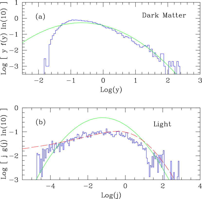
In Figure 1, we show the one-point PDFs in panel (a) and in panel (b) computed from our simulation with , a scale which is small enough to be sensitive to the local galaxy formation environment but large enough for the simulation to be accurately representing physical values. Since our binning is done in , the plotted histogram actually corresponds to [], and similarly for . Note the difference in the scales of the abscissas of the two panels.
The solid curves plotted over the histogram in both panels are log-normal distribution with the variance parameter computed from the same simulation, for dark matter and for light. The agreement between the computed dark matter PDF and the log-normal distribution is reasonably good. The departure in our computation, especially at small , is ascribed to the limited box-size of our simulation. Note that the light PDF strongly deviates from the log-normal distribution. (The long-dashed line in Figure 1(b) will be explained in Section 2.3.)
2.3 Relation between and
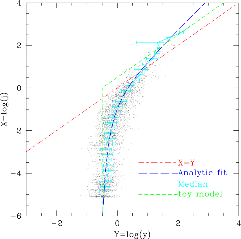
Figure 2 shows the light density parameter against the dark matter density parameter . 111We note that a similar figure was reported by Blanton et al. (1999) from our earlier simulations, but they used stellar mass density instead of . The figure was also truncated at . The simulation box-size we use here is smaller than that Blanton et al. used, and does not contain massive clusters that show the suppression of luminosity density at the highest mass density region. The point in the figure represents mass and light contained in each sphere. The solid line shows the median value in each bin, with error bars in -direction being the quartiles on both sides. The long-short dashed line shows the identical regression , and the long-dashed line shows an empirical fit to the simulation data:
| (5) |
The parameter corresponds to an effective cutoff of the mass density, below which the sphere does not contain any galaxies that emit light. The figure indicates that , i.e., the region of mass density smaller than 1/3 of the mean is dark. This dark region occupies approximately 60% of the volume when smoothed with a tophat sphere of , and contains a fraction of the total mass (these fractions are larger for voids that are operationally defined in observations: these numbers will be derived in Section 2.4). This is identified as the “void phenomenon” in the CDM universe. Luminous galaxies reside only in the dense regions. Sub-luminous galaxies prefer to lie in relatively low density regions, but the sharp increase of at around means that they live only in the edge of the voids, certainly not in the middle of the voids. These trends seem to be qualitatively consistent with the observed void phenomenon (Peebles, 2001).
Given the relation between and in Equation (5), and assuming a log-normal distribution for which is specified by , one can compute the PDF of light via . The long-dashed curve given in Figure 2 is a fit by , , and for the range (the actual value of is smaller than because of the slow asymptotic nature of the curve near the critical value). The result of thus obtained is shown as the long-dashed line in Figure 1 (b). The agreement between this model calculation and the simulation is good, verifying the self-consistency between the two PDFs in Figure 1 and the relation between given in Equation (5).
We note that there are two constraints on ,
| (6) |
The empirical fit we adopted in Equation (5) alone does not satisfy the first constraint of (6); we must add the zero luminosity component, i.e., a Dirac delta function . Hence the function should be written as
| (7) |
and the first constraint reads
| (8) |
where corresponds to the light-emitting component discussed above, i.e., the long-dashed line or the histogram itself in Figure 1 (b). We find (see Section 2.4) and that the two constraints are satisfied for the model curve within an accuracy of where we limit the integral to , the shot-noise limit of our simulation. Needless to say, the simulation data automatically satisfy the constraints by the definition of PDFs.
2.4 Distribution of Matter and Light
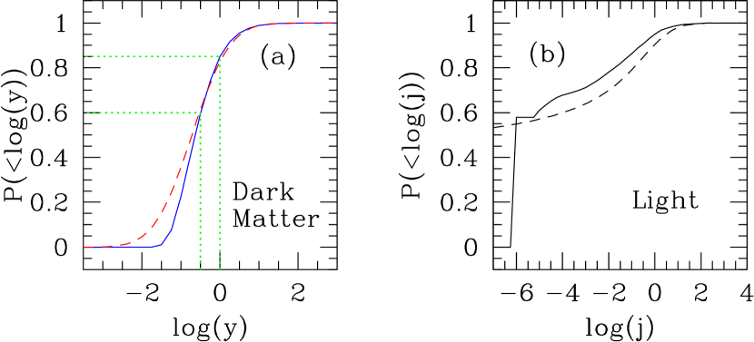
In this subsection, we study the distribution of mass and light from different angles and consider the relation to observations. Figure 3(a,b) shows the cumulative volume fraction of regions with mass density and with light density , respectively; i.e., the probability [] that a volume element has mass (light) density less than a given value of () in the abscissa. The solid line is computed from the simulated PDF, and the short-dashed line is obtained by integrating the model curve of Figure 1. We have seen that no luminous objects are present in the region of .
Figure 3(a) shows that few regions are emptier than : i.e., the ”voids”, while they are completely dark, are not thoroughly devoided in mass (cf. Peebles, 2001). From this figure we see that the region with occupies 60% of the volume (dotted line).
We see in Figure 3(b) that the light density exhibits a smooth distribution until it shows a jump at the faint end. The magnitude of the jump at (solid line) means that spheres in 60% of volume contains no light; hence the value of in Equation (7) is determined to be . The lower limit of is an artifact of the resolution of the simulation, but we consider that the realistic cutoff as determined by the Jeans and cooling conditions is rather close to this limit. The flattened distribution of towards the low luminosity end indicates that such a jump is present in reality.
Let us consider voids defined in observations. Most surveys sample galaxies down to about 4 mag below . By integrating a standard Schechter luminosity function (approximately , , and ) from (i.e. magnitude limit of ) to infinity, we expect that a sphere of radius contains 0.4 galaxies (here we assume for simplicity). This means that a sphere of luminosity cannot be observed in current standard galaxy surveys. Since the luminosity in a sphere of with the above Schechter function (with a magnitude limit of ) is , the observational threshold of light density parameter is , or using Figure 2. Namely, spheres in the region of are observed as ‘dark’. Using Figure 3(a) this means that 85% of volume is identified as voids (dotted line).
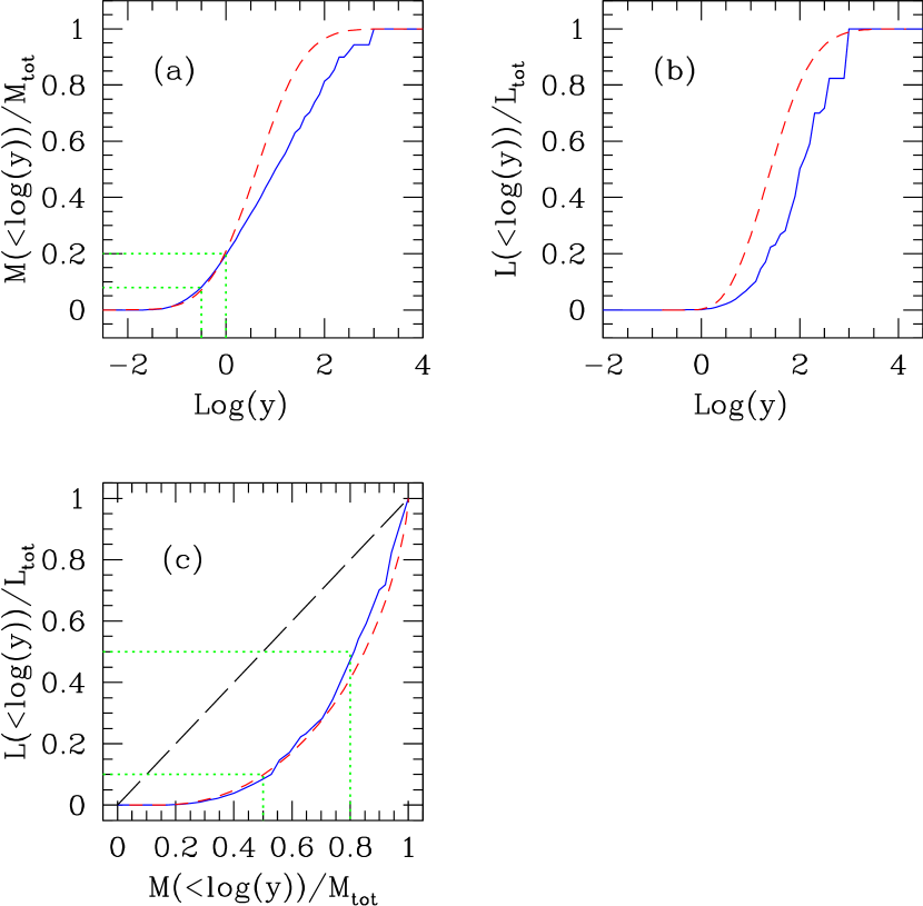
In order to see the mass in voids, we plot in Figure 4 (a) the mass fraction and (b) light fraction that are contained in regions of , i.e., and for dark matter and light, respectively. Again, the solid line is computed from the simulated PDF, and the short-dashed line is from the model curve. The result is robust against the change in the lower limit of the integration. The discrepancy between the short-dashed line and the solid line is due to the difference in the shape of the simulated and the model PDFs.
From Figure 4(a) we read that 8% of mass (corresponding to where the sharp cutoff was observed in Figure 1 ) does not emit light at all, and observationally defined voids () contain 20% of the total mass as indicated by the dotted lines. The relation between the mass fraction and the light fraction is represented more clearly in Figure 4(c), which indicates that 90% of light comes from higher density regions where 50% of mass is contained (or in other words, only 10% of light is contained in lower density region where 50% of mass is contained; see dotted lines). The departure from the diagonal line in panel (c) shows the difference in the manner that dark matter and light are distributed in the universe.
3 Applications
3.1 Mass-to-Light Ratio
The result we have seen in the preceding section indicates that the conventional evaluation of the the mass density from the luminosity density and the mean mass-to-light ratio , as (Peebles, 1971), underestimates the true value.
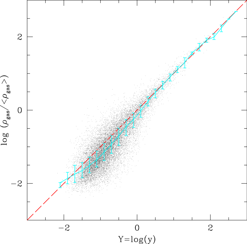
If galaxy formation is considered as largely a local process, then it is expected to be primarily a function of local gas density and gas temperature. To a first approximation baryonic gas density should roughly trace the total mass density, and indeed this is verified in our hydrodynamic simulation as shown in Figure 5. Therefore, let us assume that galaxy formation is primarily a function of only the total mass density . Namely, we take the normalized light density and the local mass-to-light ratio as functions of .
The volume averaged mean mass density can be calculated by
| (9) |
and the volume averaged mean light density is
| (10) |
So the appropriate global mean mass-to-light ratio would be
| (11) |
which is defined so that, by construction,
| (12) |
In observations one cannot observe the dark matter directly, and therefore, one samples only where the light is. This could lead to an underestimate of mass since volume elements in the universe are not treated equally. If we evaluate observationally, , by studying only those regions which emit light and weight them by the emitted light , then we are effectively evaluating the integral
| (13) | |||||
| (14) |
To see how much underestimate could be caused by weighting by light, take the following simple model in which we assume that the mass-to-light ratio is constant () in the galaxy forming regions. Namely we assume that the light density is linearly proportional to the mass density, but that there are empty voids:
| (15) |
This toy model is shown as short-dashed line in Figure 2. The mean mass-to-light ratio we defined in Eq.(11) becomes
| (16) | |||||
| (17) |
The luminosity weighted average [Eq.(13)] then becomes simply
| (18) |
So the true volume weighted average is larger than the luminosity weighted average by a factor :
| (19) |
The ratio of the integrals in Eq.(19) is just the mass fraction in “voids” divided by that in “galaxy forming regions”. We estimated that the “voids” contain 20% of the total mass; this means that the correction factor will be . This leads to an underestimate in by the same factor.
The estimate of obtained by using and (McKay et al., 2001) from gravitational lensing shears, , should therefore be corrected to give , in good agreement with the value from the WMAP experiment: (Spergel et al., 2003). The same correction also applies to similar estimates done to date, which always show rather small values of compared to the estimate of WMAP. For example an estimate of Bahcall et al. (2000), , using mass-to-light ratio as a function of scale is modified to after the correction. Similarly a low value of obtained by Fukugita, Hogan, & Peebles (1998, equation (28)) based on galaxy luminosities should also receive an upward 25% correction.
If the light PDF is estimated directly from the observation, one can numerically integrate the relation to obtain using a cosmological simulation. With one can easily obtain the mass-to-light function and the correction factor
| (20) |
3.2 Cosmic Virial Theorem
Let us now turn to the application to the “cosmic virial theorem”. Peebles (1980, 1993) shows that, if one assumes that galaxies trace mass, the “cosmic virial theorem” which relates the relative velocity dispersion and the mean mass density can be approximated by
| (21) |
To derive this equation, is assumed, where is the galaxy-galaxy correlation function, and is the galaxy-mass cross-correlation function.
As we showed earlier, galaxies do not trace mass well. Therefore if instead one were to use the galaxy-mass cross-correlation function in deriving the above relation, the value of would have been larger or smaller by a factor of
| (22) |
where is measured in units of and the right-hand-side of Eq. (21) is measured at .
The values of and are observationally known (, ) and and can be estimated in the linear regime as follows:
| (23) | |||||
| (24) | |||||
| (25) | |||||
| (26) |
where we have assumed a relation
| (27) |
and therefore,
| (28) |
The analytic fit that we adopted in § 2.3 Eq. (5) implies for the domain of that concerns us. By comparing Eq. (26) and the original functional form for , one obtains
| (29) |
For any value of larger than unity will therefore gives
| (30) |
Using these relations in Eq. (22), the matter density of the universe estimated by Peebles by this method () should be increased by a factor of , which yields a corrected value of . The agreement with the WMAP result is improved by this correction.
4 Discussion and Conclusions
Very little work has been done on the optical probability distribution function (PDF): the probability of finding a region (of some given size) containing a specified range of optical light output from galaxies within that region. Even less has been done in relating the optical PDF with the matter (or dark matter) PDF.
What is known is that the low density regions (optical “voids”) are relatively unpopulated by galaxies (Kirshner et al., 1981; Rood, 1988), and consequently are optically faint as compared from the dark matter simulations of the currently popular concordance model. If this is correct, then “bias” — the ratio of galaxies to dark matter — is different in high and low density regions. And more seriously, our observational tracers of cosmic structure are giving us a view of the universe that is inherently contaminated by selection bias.
We compute the effects in a TVD cosmic hydrodynamic simulation and then estimate the error that would have been involved, had these simulations been observed and analyzed using conventional techniques. Focusing on the global value of (which of course is known for the simulated universe), we can estimate the corrections, and when applying these corrections we obtain increased values of to the range , which is in better accord with the CMB determinations.
The relation between mass PDF and light PDF also gives us insight concerning the nature of the void phenomenon, and enables us to estimate the mass and volume fractions occupied by voids. Our result indicates that no galaxies can be present in the middle of voids: sub-luminous galaxies are distributed in the edge of voids, whereas luminous galaxies reside only in high-density filaments. The quantitative basis for these statements will be presented in a subsequent paper, but the concept is as follows. A large void can be considered as a small piece of a lower density universe. The implies a shift to a lower characteristic halo mass in such regions and a shift in the horizontal scale in Figures (2) and (3a) to domains in which galaxy formation is less efficient. At the centers of such voids all galaxy formation is suppressed and at the edges high luminosity galaxies (from higher mass halos) are suppressed more than lower luminosity systems. A recent numerical study by Gottlöeber et al. (2003) supports this view.
Future work using large-scale surveys can provide the empirical data needed to compute the optical PDF properly. When this is combined with detailed numerical simulations of the dark matter, we will be able to self-consistently evaluate these effects better and use the so determined relation between light density and mass density in our analysis of observational data.
References
- Bahcall et al. (2000) Bahcall, N. A., Cen, R., Davé, R., Ostriker, J. P., & Yu, Q. 2000, ApJ, 541, 1
- Benson, et al. (2003) Benson, A., Hoyle, F., Torres, F., Vogeley, M. S., 2003, MNRAS, 340, 160
- Blanton et al. (1999) Blanton, M., Cen, R., Ostriker, J. P., Strauss, M. A., 1999, ApJ, 522, 590
- Bruzual & Charlot (1993) Bruzual, A. G. & Charlot, S., 1993, ApJ, 405, 538
- Cen & Ostriker (1993) Cen, R., & Ostriker, J.P. 1993, ApJ, 417, 404
- Cen et al. (2002) Cen, R., Ostriker, J. P., Prochaska, J. X., & Wolfe, A. M., 2002, preprint (astro-ph/0203524)
- Coles & Jones (1991) Coles, P. & Jones, B. 1991, MNRAS, 248, 1
- Dekel & Lahav (1999) Dekel, A. & Lahav, O. 1999, ApJ, 520, 24
- Efstathiou et al. (1990) Efstathiou, G. et al. 1990, MNRAS, 247, 10
- Fukugita, Hogan, & Peebles (1998) Fukugita, M., Hogan, C. J., & Peebles, P. J. E. 1998, ApJ, 503, 518
- Gottlöeber et al. (2003) Gottlöeber, S., Lokas, E., Klypin, A., Hoffman, Y. 2003, MNRAS, submitted (astro-ph/0305393)
- Kayo, Taruya, & Suto (2001) Kayo, I., Taruya, A., & Suto, Y. 2001, ApJ, 561, 22
- Kirshner et al. (1981) Kirshner, R. P., Oemler, A., Jr., Schechter, P. L., & Shectman, S. A., 1981, ApJ, 248, L57
- Kofman et al. (1994) Kofman, L., Bertschinger, E., Gelb, J. M., Nusser, A., & Dekel, A. 1994, ApJ, 420, 44
- McKay et al. (2001) McKay, T. A. et al., preprint astro-ph/0108013
- Nagamine (2002) Nagamine, K. 2002, ApJ, 564, 73
- Nagamine, Fukugita, Cen, & Ostriker (2001b) Nagamine, K., Fukugita, M., Cen, R., & Ostriker, J. P. 2001, MNRAS, 327, L10
- Nagamine, Fukugita, Cen, & Ostriker (2001a) Nagamine, K., Fukugita, M., Cen, R., & Ostriker, J. P. 2001, ApJ, 558, 497
- Peebles (1971) Peebles, P. J. E. 1971, Physical Cosmology, Princeton University Press, Princeton, New Jersey
- Peebles (1980) Peebles, P. J. E. 1980, The Large-Scale Structure of the Universe, Princeton University Press, Princeton, New Jersey, § 74
- Peebles (1993) Peebles, P. J. E. 1993, Principles of Physical Cosmology, Princeton University Press, Princeton, New Jersey, p.481
- Peebles (2001) Peebles, P. J. E. 2001, ApJ, 557, 495
- Rood (1988) Rood, H. J., 1988, ARA&A, 26, 245
- Ryu et al. (1993) Ryu, D., Ostriker, J. P., Kang, H., Cen, R. 1993, ApJ, 414, 1
- Sigad, Branchini, & Dekel (2000) Sigad, Y., Branchini, E., Dekel, A. 2000, ApJ, 540, 62
- Spergel et al. (2003) Spergel, et al. 2003, ApJ, accepted (astro-ph/0302209)
- Taylor & Watts (2000) Taylor, A. N. & Watts, P. I. R. 2000, MNRAS, 314, 92
- Vogeley, Geller, & Huchra (1991) Vogeley, M. S., Geller, M. J., & Huchra, J. P., 1991, ApJ, 382, 44
- Vogeley, et al. (1994) Vogeley, M. S., Geller, M. J., Changbom, P., & Huchra, J. P., 1994, ApJ, 108, 745
