Gravitational Lensing by Large Scale Structures:
A Review

Abstract

We review all the cosmic shear results obtained so far, with a critical discussion of the present strengths and weaknesses. We discuss the future prospects and the role cosmic shear could play in a precision cosmology era.

Institut d’Astrophysique de Paris, 98bis Bd Arago, 75014, Paris

Institut d’Astrophysique de Paris, 98bis Bd Arago, 75014, Paris
LERMA, Observatoire de Paris, 61 av. de l’Observatoire, 75014, Paris

1. Introduction

The observation of gravitational lensing by large scale structures is a direct probe of the matter distribution in the Universe. This method gives the most unbiased picture of the matter distribution at low redshift compared to other techniques like cosmic velocity fields, galaxy distribution or Lyman-$\alpha$ forest studies. Indeed, these techniques rely on assumptions either like the dynamical stage of the structure involved, or the properties of visible material versus dark matter biasing, or suffer of a poor sampling, or a combinaison of those. On the other hand, lensing by large scale structures suffers from practical difficulties, like its sensitivity to non-linear power spectrum predictions, or to the Point Spread Function corrections, which we will discuss later. In this review, we intend to give a present day picture of the cosmic shear research and to discuss the technical issues that could be a limitation. These technical limitations will certainly be overcome sooner or later, this is why a discussion of the role of cosmic shear for precision cosmology is also of interest. Although this paper is supposed to review the topic, there are already more than hundreds of publications on the cosmic shear subject alone. It is therefore difficult to address all aspects in details, and to mention everything (theory, simulations and observations). Instead, we choose to focus on observations, data analysis and related cosmological interpretations. By cosmic shear, we mean distorsion of the distant galaxies only. The magnification aspects of gravitational lensing by large scale structures, which is only at its beginning in terms of intensive observations, will not be reviewed. We apologize whose those of which work will not be discussed.

2. Linking galaxy shapes to theory

2.1. Lensing by large scale structures

Light propagation in the inhomogeneous universe

Figure 1.: A light bundle and two of its rays $\cal L$ and $\cal L^{\prime}$. ${{\hbox{$\bf\xi$}}}(w)$ is the physical diameter distance, which separates the two rays on the sky, viewed from the observer ($w=0$).

We first have to define the homogeneous background universe notations (identical to Schneider et al. 1998). The metric of the homogeneous Universe is written in the form

$${\rm d}s^{2}=c^{2}\,{\rm d}t^{2}-a^{2}(t)\left[{\rm d}w^{2}+f_{K}^{2}(w){\rm d}\omega^{2}\right]\;,$$ (1)

where $a(t)=(1+z)^{-1}$ is the cosmic scale factor normalized to unity today, $w(z)$ is the radial coordinate, and $f_{K}(w)$ is the comoving angular diameter distance out to a distance $w(z)$. The radial distance $w(z)$ is given by the redshift integral:

$$w(z)=\int_{0}^{z}{\rm d}z^{\prime}{c\over H}={c\over H_{0}}\int_{0}^{z}{{\rm d}z^{\prime}\over\sqrt{(1+z^{\prime})^{3}\Omega_{0}+(1+z^{\prime})^{2}(1-\Omega_{0}-\Omega_{\Lambda})+\Omega_{\Lambda}}}\;,$$ (2)

where $H_{0}$ is today’s Hubble constant, and the angular diameter distance $f_{K}(w)$ reads

$$f_{K}(w)=\cases{K^{-1/2}\sin(\sqrt{K}w)&for $K>0$ ,\cr w&for $K=0$ ,\cr(-K)^{-1/2}\sinh(\sqrt{-K}w)&for $K<0$ ,\cr}$$ (3)

where $K$ is the curvature

$$K=\left({H_{0}\over c}^{2}\right)\left(\Omega_{0}+\Omega_{\Lambda}-1\right),$$ (4)

with $\Omega_{0}$ and $\Omega_{\Lambda}$ the mean density parameter and the vacuum energy today.

Consider two light rays $\cal L$ and $\cal L^{\prime}$ coming from a distant source and converging to an observer, and define ${\rm d}{{\hbox{$\bf\theta$}}}$ as the observed angular vector between the two rays (Figure1). We use the Cartesian complex coordinates, so ${\rm d}{{\hbox{$\bf\theta$}}}=({\rm d}\theta_{1},i{\rm d}\theta_{2})$. In the absence of any inhomogeneities along the line of sight, the physical distance between the two rays at an angular distance $f_{K}(w_{S})$ from the observer to the source is defined as ${{\hbox{$\bf\xi$}}}=f_{K}(w_{S})\;{\rm d}{{\hbox{$\bf\theta$}}}$. Due to the inhomogeneities, like clusters of galaxies, voids and filaments, the physical distance $\bf\xi$ deviates from this simple relation, and can be linearized as:

$${{\hbox{$\bf\xi$}}}=f_{K}(w_{S}){\cal A}\;{\rm d}{{\hbox{$\bf\theta$}}} = f_{K}(w_{S})\pmatrix{\kappa+\gamma&-i\omega\cr-i\omega&\kappa-\gamma}\;{\rm d}{{\hbox{$\bf\theta$}}}$$ (5)

$$= f_{K}(w_{S})(\kappa-i\omega)\;{\rm d}{{\hbox{$\bf\theta$}}}+f_{K}(w_{S})\gamma\;{\rm d}{{\hbox{$\bf\theta$}}}^{\star}.$$ (6)

Figure 2.: Effect of $\kappa$, $\gamma$ or $\omega$ on the displacement of two test particles $1$ and $2$ located on a test ring (dot-dashed circle) with coordinates $({\rm d}\theta,0)$ and $(0,i{\rm d}\theta)$.

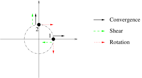
The matrix ${\bf{\cal A}}$ is by definition the amplification matrix. The geometrical origin of this expression is easily understood when drawing how ${\rm d}\theta_{1}$ and ${\rm d}\theta_{2}$ change with a small (but non-vanishing) $\kappa$, $\gamma$ or $\omega$ (see Figure 2). They are just numbers which describe the infinitesimal relative displacement of two rays $\cal L$ and $\cal L^{\prime}$.

$${\rm d}{{\hbox{$\bf\xi$}}}_{\kappa}\propto\pmatrix{\kappa\;{\rm d}\theta_{1}\cr i\kappa\;{\rm d}\theta_{2}};\;{\rm d}{{\hbox{$\bf\xi$}}}_{\gamma}\propto\pmatrix{\gamma\;{\rm d}\theta_{1}\cr-i\gamma\;{\rm d}\theta_{2}};\;{\rm d}{{\hbox{$\bf\xi$}}}_{\omega}\propto\pmatrix{\omega\;{\rm d}\theta_{2}\cr-i\omega\;{\rm d}\theta_{1}}$$ (7)

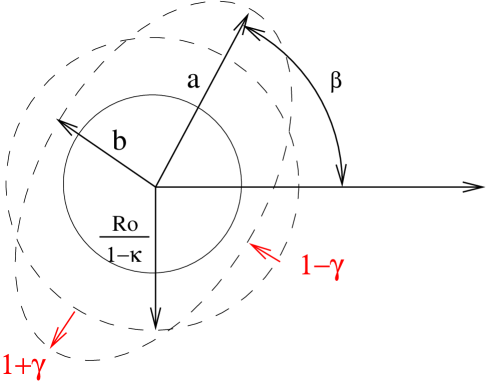
As we shall see now, they are the quantities which contain the cosmological information. By definition, $\kappa$ is called the convergence field, $\gamma$ the shear field, and $\omega$ the rotation field. When the shear is not expressed in the eigenspace (which is the case in Figure 2 for instance), $\bf\gamma$ is a complex vector in general (see Figure 3).

A light beam is a congruence of null geodesics, which are marked with respect to a fiducial (reference) geodesic having a tangent vector $k_{\mu}$. The rays $\cal L$ and $\cal L^{\prime}$ are two geodesics of the congruence, whose the separation ${{\hbox{$\bf\xi$}}}=\xi_{1}+i\xi_{2}$ is defined as a space-like vector perpendicular to the wave-vector $k_{\mu}$. As above, for an infinitesimal displacement along the congruence it is always possible to decompose the geometrical deformation of the ray bundle into a uniform expansion $\Theta$, a shear $\sigma$ and a rotation $W$. This defines the well known optic scalars (Sachs 1961):

$$\Theta={1\over 2}k^{\mu}_{;\mu}\;\ \ \ \sigma=\sqrt{{1\over 2}[k_{(\mu;\nu)}k^{\mu;\nu}-{1\over 2}(k^{\mu}_{;\mu})^{2}}\ ;\ \ \ W=\sqrt{{1\over 2}k_{[\mu;\nu]}k^{\mu;\nu}},$$ (8)

where $k_{\mu;\nu}$ is the covariant derivative of the wave-vector and $(\mu;\nu)$ and $[\mu;\nu]$ denote the symmetric and antisymmetric permutation of indices respectively. The evolution of the optic scalars along the congruence is completely determined by the optical scalar equations which depend on the gravitational field (Sachs 1961):

$${d(\Theta+iW)\over d\lambda}+(\Theta+iW)^{2}+|\sigma|^{2}={\cal R}={1\over 2}R_{\mu\nu}k^{\mu}k^{\nu}$$

$${d\sigma\over d\lambda}+\sigma\Theta={\cal F}=C_{\mu\alpha\nu\beta}k^{\mu}k^{\nu}\bar{t}^{\alpha}\bar{t}^{\beta}.$$ (9)

Here, the geodesic is parametrized with ${\rm d}\lambda={\rm d}w/(1+z)^{2}$. $R_{\mu\nu}$ and $C_{\mu\alpha\nu\beta}$ are the Ricci and the Weyl tensors respectively. $t^{\alpha}$ is the complex null tetrad (or Sachs tetrad) such that $t^{\alpha}k_{\alpha}=0$ and $\bar{t}_{\alpha}t^{\alpha}=1$. Note that the first equation in (9) is nothing else but the Raychaudhuri equation for null geodesics.

For an infinitesimal displacement along the congruence, the separation $\bf\xi$ transforms according to Eq.(6):

$${d{{\hbox{$\bf\xi$}}}\over d\lambda}=(\Theta-iW){{\hbox{$\bf\xi$}}}+\sigma{{\hbox{$\bf\xi$}}}^{\star}.$$ (10)

Differentiating Eq.(10) and substituting Eq.(9) leads to the evolution equation of $\bf\xi$ along the congruence as a function of the gravitational fields ${\cal R}$ and ${\cal F}$:

$${d^{2}{{\hbox{$\bf\xi$}}}\over d\lambda^{2}}=\pmatrix{{\cal R}-Re({\cal F})&iIm({\cal F})\cr iIm({\cal F})&{\cal R}+Re({\cal F})}{{\hbox{$\bf\xi$}}}.$$ (11)

The final step is to calculate $\cal R$ and $\cal F$ from the Ricci and the Weyl tensors for a Newtonian gravitational potential $\Phi$. Straightforward but lengthy calculations give:

$${\cal R}=-{1\over a^{2}(w)}\Delta\Phi\ ;\ \ \ {\cal F}=-{1\over a^{2}(w)}(\partial_{1}^{2}\Phi-\partial_{2}^{2}\Phi+2i\partial_{1}\partial_{2}\Phi),$$ (12)

where $a(w)$ is the scale factor of the unperturbed background metric, and $w$ the radial distance. Using a perturbative expansion for the amplification matrix ${\cal A}_{ij}={\cal A}^{(0)}_{ij}+{\cal A}^{(1)}_{ij}+...$ and for the gravitational potential $\Phi=\Phi^{(1)}+\Phi^{(2)}+...$, Eq.(11) can be solved iteratively. The homogeneous universe case corresponds to ${\cal A}_{ij}={\cal A}^{(0)}_{ij}=\delta_{ij}$ and $\Phi=0$. It is then easy to obtain the general first order solution for the amplification matrix in the direction $\bf\theta$:

$${\cal A}_{ij}({{\hbox{$\bf\theta$}}})=\delta_{ij}+{\cal A}^{(1)}_{ij}({{\hbox{$\bf\theta$}}})=\delta_{ij}-{2\over c^{2}}\int_{0}^{w_{S}}{\rm d}w\;{f_{K}(w-w^{\prime})f_{K}(w^{\prime})\over f_{K}(w)}\Phi^{(1)}_{,ij}(f_{K}(w^{\prime}){{\hbox{$\bf\theta$}}},w^{\prime}),$$ (13)

where $w_{S}$ is the position of the source. Eq.(13) is the basic lensing equation used to calculate the distortion and the magnification of distant sources. This result is a first order expression and is only valid in the realm of the Born approximation where the lensing properties are calculated along the unperturbed light path (of direction $\bf\theta$). Therefore, all contribution coming from the lens-lens coupling are neglected. For most practical applications this is however an excellent approximation (Bernardeau et al. 1997, Schneider et al. 1998), as we shall see later.

Back to the lensing effects (Eq.6), the geometrical deformation of a light bundle can be expressed as an integrated effect along the line-of-sight:

$$\kappa=1+{1\over 2}Tr({\cal A}^{(1)}_{ij})\ ;\ \ \ \gamma={1\over 2}({\cal A}^{(1)}_{11}-{\cal A}^{(1)}_{22}+2i{\cal A}^{(1)}_{12})\ ;\ \ \ \omega=0.$$ (14)

These expressions show that a scalar perturbation will never induce a rotation of the light bundle at the first order ($\omega=0$). Figure 3 shows the effect of cosmic shear on a distant circular galaxy, at the first order ($\kappa\;\ll\;1$ and $\gamma\;\ll\;1$). It shows that the shear can be obtained from the measurement of the shape of galaxies. The practical methods to do this measurement will be discussed in Section 2.2.

Figure 3.: Illustration of the first order effect of cosmic shear on a circular background galaxy of radius $R_{0}$. The convergence is an isotropic distortion of the image of the galaxy, while the shear is an anisotropic distortion.

Mean fields

The second order derivatives of the gravitational potential field can be written as function of the mass density contrast $\delta$, using the Poisson equation:

$$\nabla^{2}\Phi={3H_{0}^{2}\Omega_{\rm 0}\over 2a}\delta.$$ (15)

From Eq(13), we get the convergence $\kappa({{\hbox{$\bf\theta$}}})$ in the direction $\bf\theta$, as function of $\delta$, integrated along the line of sight:

$$\kappa({{\hbox{$\bf\theta$}}},w)={3\over 2}{H_{0}\over c}^{2}\Omega_{\rm 0}\int_{0}^{w_{S}}{\rm d}w^{\prime}\;{f_{K}(w-w^{\prime})\,f_{K}(w^{\prime})\over f_{K}(w)}{\delta\left(f_{K}(w^{\prime}){\hbox{$\bf\theta$}},w^{\prime}\right)\over a(w^{\prime})},$$ (16)

with similar (but not identical) expressions for ${{\hbox{$\bf\gamma$}}}({{\hbox{$\bf\theta$}}})$. The sources have been assumed to be at a single ’redshift’ $w_{S}$, but similar expressions can be easily generalized for a more realistic redshift distribution. In that case, the lensing fields are integrated along the redshift with the proper source distribution $p_{w}(w){\rm d}w$ from $0$ to the horizon $w_{\rm H}$:

$$\kappa({{\hbox{$\bf\theta$}}})={3\over 2}\left(H_{0}\over c\right)^{2}\Omega_{\rm 0}\int_{0}^{w_{\rm H}}{\rm d}w\;g(w)\,f_{K}(w){\delta\left(f_{K}(w){\hbox{$\bf\theta$}},w\right)\over a(w)},$$ (17)

with

$$g(w)=\int_{w}^{w_{\rm H}}{\rm d}w^{\prime}\;p_{w}(w^{\prime})\,{f_{K}(w^{\prime}-w)\over f_{K}(w^{\prime})}.$$ (18)

Limber equation and small angle approximation

We are primarily interested in the statistical properties of the lensing fields, which are given by the moments of the field. The variance is the first non trivial moment; its evolution with angular scale depends on cosmological parameters and on the geometrical properties of the Universe due to the light rays propagation. The mass density power spectrum $P_{3D}(k)$ is defined as

$$\langle\tilde{\delta}({\bf k})\tilde{\delta}^{*}({\bf k}^{\prime})\rangle=(2\pi)^{3}\delta_{\rm D}({\bf k}-{\bf k}^{\prime})\,P_{3D}(k,w).$$ (19)

Likewise, one can define the convergence power spectrum $P_{\kappa}(s)$:

$$\langle\tilde{\kappa}({\hbox{$\bf s$}})\tilde{\kappa}^{*}({\hbox{$\bf s$}}^{\prime})\rangle=(2\pi)^{2}\delta_{\rm D}({\bf s}-{\bf s}^{\prime})\,P_{\kappa}(s).$$ (20)

The time dependence in Eq(19) stands for the growth of structures. For an EdS Universe, it can be factorized, but in the general case it is more complicated, in particular in the non-linear regime where time dependence and scales are coupled. The jump from the 3-D wave vector ${\bf k}$ to the 2-D angular wave vector ${\bf s}$ is ensured from the line of sight integration using the Limber approximation (Limber, 1954). To simplify Eq(17), it can be written as $\kappa({{\hbox{$\bf\theta$}}})=\int{\rm d}w\;q(w)\;\delta(f_{K}(w){\hbox{$\bf\theta$}},w)$. In real space, the convergence correlation function $\xi_{\kappa}(\Delta{{\hbox{$\bf\theta$}}})=\langle\kappa({{\hbox{$\bf\theta$}}})\kappa({{\hbox{$\bf\theta$}}}+\Delta{{\hbox{$\bf\theta$}}})\rangle$ can be eventually computed (Kaiser 1998):

$$\langle\kappa({{\hbox{$\bf\theta$}}})\kappa({{\hbox{$\bf\theta$}}}+\Delta{{\hbox{$\bf\theta$}}})\rangle = \int{\rm d}w\;q(w)\int{\rm d}w^{\prime}\;q(w^{\prime})\;\langle\delta(f_{K}(w){\hbox{$\bf\theta$}},w)\delta(f_{K}(w^{\prime})({\hbox{$\bf\theta$}}+\Delta{{\hbox{$\bf\theta$}}}),w^{\prime})\rangle$$ (21)

$$\simeq \int{\rm d}w\;q^{2}(w)\int{\rm d}w^{\prime}\;\langle\delta(f_{K}(w){\hbox{$\bf\theta$}},w)\delta(f_{K}(w^{\prime})({\hbox{$\bf\theta$}}+\Delta{{\hbox{$\bf\theta$}}}),w^{\prime})\rangle,$$ (22)

assuming that the selection function $q(w)$ does not vary across the largest fluctuations of the density and that the fluctuations are much smaller than the distance of the sources. In order to express all cosmic shear 2-points statistics, we are in fact interested in the convergence power spectrum $P_{\kappa}(s)$:

$$P_{\kappa}(s)=\int{\rm d}{{\hbox{$\bf\theta$}}}\;\xi_{\kappa}({{\hbox{$\bf\theta$}}})\;{\rm e}^{-i{\bf s}\cdot{{\hbox{$\bf\theta$}}}}.$$ (23)

The density contrast $\delta(f_{K}(w){\hbox{$\bf\theta$}},w)=\delta({\bf r})$ can be expressed in Fourier space:

$$\delta({\bf r}) = \int{{\rm d}{\bf k}\over(2\pi)^{3}}\;{\rm e}^{-i{\bf k}\cdot{\bf r}}\;\tilde{\delta}({\bf k},w)$$ (24)

$$= \int{{\rm d}{\bf k}\over(2\pi)^{3}}\;{\rm e}^{-i{\bf k}_{\perp}\cdot{{\hbox{$\bf\theta$}}}\;f_{K}(w)}\;{\rm e}^{-i\;k_{3}w}\;D_{1}^{(+)}(w)\;\tilde{\delta}({\bf k}),$$ (25)

where $D_{1}^{(+)}(w)$ is the linear structure growth factor (see the next section non-linear power spectrum), and ${\bf k}=({\bf k}_{\perp},k_{3})$, ${\bf k}_{\perp}$ is the wave-vector perpendicular to the line of sight. From this equation and Eq(19), one can express the density correlation function appearing in Eq(22):

$$\langle\delta({\bf r})\delta^{\star}({\bf r}^{\prime})\rangle = \int{\rm d}{\bf k}\;{\rm e}^{-i{\bf k}_{\perp}\cdot{{\hbox{$\bf\theta$}}}\;f_{K}(w)}\;{\rm e}^{i{\bf k}_{\perp}\cdot({{\hbox{$\bf\theta$}}}+\Delta{{\hbox{$\bf\theta$}}})\;f_{K}(w^{\prime})}$$ (26)

$$\times {\rm e}^{-i\;k_{3}(w-w^{\prime})}\;D_{1}^{(+)}(w)D_{1}^{(+)}(w^{\prime})\;P_{3D}(k).$$ (27)

When, as in our case, the small angle approximation is valid ( $|\Delta{{\hbox{$\bf\theta$}}}|\leq 1-2\;{\rm degrees}$), the transverse wave-vector ${\bf k}_{\perp}$ carries most of the power at $|{\bf k}|$; that is $P_{3D}(k)\simeq P_{3D}(k_{\perp})$ (Peebles 1980). The $k_{3}$ integration then gives a Dirac delta function $\delta_{D}(w-w^{\prime})$. If we perform the variable change ${\bf k}_{\perp}\;f_{K}(w)={\bf s}$ the convergence power spectrum becomes:

$$P_{\kappa}(s)=\int{\rm d}w\;{q^{2}(w)\over f_{K}^{2}(w)}\left[D_{1}^{(+)}(w)\right]^{2}\;P_{3D}\left({s\over f_{K}(w)}\right).$$ (28)

Back to the notations of Eq(17), the convergence power spectrum finally writes

$$P_{\kappa}(s)={9\over 4}\left(H_{0}\over c\right)^{4}\Omega_{\rm 0}^{2}\int_{0}^{w_{\rm H}}{\rm d}w\;{g^{2}(w)\over a^{2}(w)}P_{3D}\left({s\over f_{K}(w)};w\right).$$ (29)

The shear power spectrum $P_{\gamma}(s)$ is identical to this expression. The reason is that, in Fourier space, the quantities $\langle\tilde{\kappa}^{2}\rangle$ and $\langle|\tilde{{\hbox{$\bf\gamma$}}}|^{2}\rangle$ are identical. This can be derived easily from Eq(13) and Eq(14), with the derivatives replaced by powers in ${\bf s}$’s in Fourier space. As we shall see, this allows us to extract the convergence 2-points statistics directly from the data. Higher order statistics is a more difficult issue which will be discussed later.

Non-linear power spectrum

The normalization of the mass density power spectrum $P_{3D}$ is defined in the conventional way, by computing the mass density variance within a sphere of $8\;{\rm h}^{-1}{\rm Mpc}$ radius at redshift zero:

$$\sigma_{8}^{2}=\langle\delta_{R}^{2}\rangle={1\over 2\pi^{3}}\int d{\bf k}P_{3D}(k,0)|W(kR)|^{2},$$ (30)

where $W(kR)={3\over(kR)^{2}}\left({\sin(kR)\over kR}-\cos(kR)\right)$ is the Fourier transform of the top-hat window function of radius $R$. The transition from the linear to the non-linear scales is identified by $\sigma_{8}\sim 1$. In the linear regime, where the density contrast of the mass distribution is low ($\delta\;\ll\;1$), the fluid equations describing the structure growth can be solved perturbatively, and one obtains for the growing mode:

$$P_{3D}(k,w)=\left[D^{(+)}_{1}(w)\right]^{2}\;P_{3D}(k),$$ (31)

with,

$$D^{(+)}_{1}(w)={5\over 2}\;\Omega_{0}\;H(w)\;\int_{0}^{w}\;{{\rm d}a\over a^{3}\;H(a)}.$$ (32)

Figure 4.: The left panel is a 3-dimensional mass power spectrum for the linear (dashed) and non-linear (solid, using Smith et al. 2002) regimes when baryons are included. A value of $\Omega_{b}=0.05$ was used. The right panel shows the induced convergence power spectrum (Eq.29) for the two dynamical regimes. Other parameters are $\Omega_{\rm cdm}=0.25,\Omega_{\Lambda}=0.7,\sigma_{8}=0.9,h=0.7,z_{\rm source}=0.8$.

In the non-linear regime, the structure growth cannot be solved analytically and its description must rely on non-linear models (Peacock & Dodds, 1996, Smith et al. 2002), following an original idea of Hamilton et al. (1991). Non-linear predictions of the matter power spectrum are performed from the knowledge of the spatial 2-points correlation function of the galaxies $\xi_{2}({\bf r})={V\over(2\pi)^{3}}\int\;{\rm d}{\bf k}\;P(k)\;e^{-i{\bf k}\cdot{\bf r}}$. An accurate measurement of $\xi_{2}({\bf r})$ is given for instance by the 2dF (Percival et al. 2001) or the SDSS surveys (Dodelson, S., et al. 2002):

$$\xi_{2}(r)=\left({r_{0}\over r}\right)^{\gamma},$$ (33)

with $r_{0}=4.3\pm 0.3\;h^{-1}{\rm Mpc}$ and $\gamma=1.71\pm 0.06$. The stable clustering hypothesis stipulates that at very small scales (strong non-linear regime), the internal profile of clusters of galaxies remain constant with time for any cosmological model, and that the cluster distribution is driven by the cosmic expansion. This means that the correlation function is fixed in proper coordinates, but its amplitude evolves as a volume effect like $(1+z)^{-3}$. At large scale (linear regime), the correlation function follows the perturbation theory. Since the correlation function $\xi_{2}(r)$ behaves like $r^{-\gamma}$ for any cosmological model, we therefore have the two following limiting cases (Peacock 1999):

$$\xi_{2}(r,z)\propto(1+z)^{\gamma}(1+z)^{-3}\ \ \ {\rm non-linear}$$ (34)

$$\xi_{2}(r,z)\propto\left[D^{(+)}_{1}(w)\right]^{2}\ \ \ {\rm linear}$$ (35)

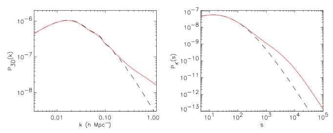
A mapping from the linear to the non-linear scale has been conjectured (Hamilton et al. 1991, Peacock & Dodds 1996, Smith et al. 2002), and calibrated using N-body simulation. The transition from linear to non-linear scales is described by a few slowly varying functions that depend on cosmological parameters. The same argument applies to the 3-D power spectrum, which is needed for cosmic shear predictions down to small scales (Eq.29) (Peacock & Dodds 1994). Figure 4 is an example of 3-dimensional and convergence power spectra in the linear and non-linear regimes. A fair amount of baryons was included (using CAMB, Lewis et al. 2002), in order to show that the baryon oscillations, which are clearly visible on the 3D spectrum, are severely diluted in the projected spectrum.

2-points statistics

Figure 5.: In order to compute the shear variances, the galaxy ellipticities are smoothed within a window (dashed red) of fixed radius $\theta_{c}$ (left). The shear variance will show up as an excess of galaxy alignment with respect to random orientation. The right panel shows the profile of the two filters one usually consider, top-hat (solid line) and compensated (dashed line). On the left, the axis $(e_{t},e_{r})$ correspond to the local frame attached to each individual galaxy, on which the galaxy ellipticity components can be projected out to give an estimate of the tangential $\gamma_{t}$ and radial shear $\gamma_{r}$.

In practice, the variance of the convergence (or shear, which is the same) is computed within a given smoothing window $U({{\hbox{$\bf\theta$}}})$ of radius $\theta_{c}$, which can be written:

$$\langle\kappa^{2}\rangle_{\theta_{c}} = \langle\left(\int{\rm d}^{2}\theta^{\prime}\;U(\theta^{\prime})\kappa(\theta^{\prime})\right)^{2}\rangle$$ (36)

$$= \int{\rm d}^{2}\theta^{\prime}\;U(\theta^{\prime})\int{\rm d}^{2}\vartheta\;U(\vartheta)\langle\kappa({{\hbox{$\bf\theta$}}}^{\prime})\kappa({{\hbox{$\bf\vartheta$}}})\rangle.$$ (37)

If we express the convergence from its Fourier transform $\kappa({{\hbox{$\bf\theta$}}})=\int{\rm d}^{2}{\bf s}\;\tilde{\kappa}({\bf s})\;{\rm e}^{i{{\hbox{$\bf\theta$}}}\cdot{\bf s}}$ and using Eq(20), we obtain:

$$\langle\kappa^{2}\rangle_{\theta_{c}} = \int{\rm d}^{2}\theta^{\prime}\;U(\theta^{\prime})\int{\rm d}^{2}\vartheta\;U(\vartheta)\int{{\rm d}^{2}s\over(2\pi)^{2}}\;{\rm e}^{i{\bf s}\cdot({\hbox{$\bf\theta$}}^{\prime}-{{\hbox{$\bf\vartheta$}}})}P_{\kappa}(s)$$ (38)

$$= 2\pi\int_{0}^{\infty}{\rm d}s\;s\,P_{\kappa}(s)\left(\int_{0}^{\theta_{c}}{\rm d}\vartheta\;\vartheta\,U(\vartheta)\,{\rm J}_{0}(s\vartheta)\right)^{2}.$$ (39)

This expression is general, and can be applied to any smoothing window $U({{\hbox{$\bf\theta$}}})$. Since $P_{\gamma}(s)=P_{\kappa}(s)$, it also expresses the shear variance $\langle\gamma^{2}\rangle_{\theta_{c}}$. As illustrated in Figure 5 , we are primarily interested in a top-hat filtering, for which,

$$\langle\gamma^{2}\rangle={2\over\pi}\int{\rm d}s\;s\;P_{\kappa}(s)\left[{J_{1}(s\theta_{c})\over s\theta_{c}}\right]^{2},$$ (40)

and in the compensated filtering having $\int_{0}^{\theta_{c}}{\rm d}\theta\;\theta\;U(\theta)=0$ (zero mean). The choice of $U(\theta)$ is arbitrary, provided it has a zero mean. Here we use the expression (Schneider et al. 1998):

$$U(\theta)={9\over\pi\theta_{c}^{2}}\left(1-\left({\theta\over\theta_{c}}\right)^{2}\right)\left({1\over 3}-\left({\theta\over\theta_{c}}\right)^{2}\right),$$ (41)

so the variance of the convergence with this filter is:

$$\langle M_{\rm ap}^{2}\rangle={288\over\pi}\int{\rm d}s\;s\;P_{\kappa}(s)\left[{J_{4}(s\theta_{c})\over s^{2}\theta_{c}^{2}}\right]^{2}.$$ (42)

Figure 6.: Top-hat (dashed line) and compensated (solid line) filters in Fourier space. This plot illustrates the fact that the compensated filter is a pass-band filter, and therefore is a broad-band estimates of the convergence power spectrum in real space.

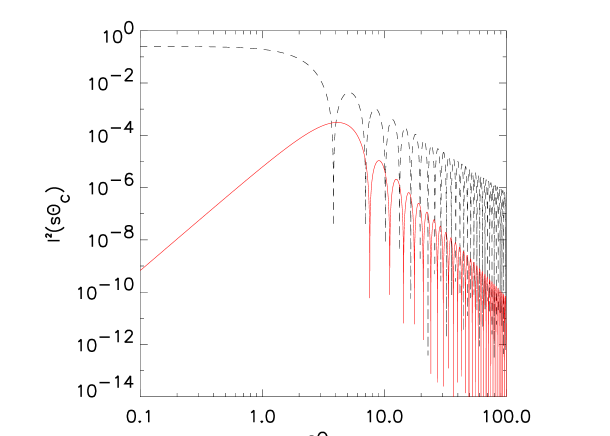
The nice feature of the compensated filter is that it is a pass-band filter, which means that the variance Eq(42) is a direct estimate of the convergence power spectrum in real space. Note that the power is estimated around $s\sim\;5/\theta_{c}$. Furthermore, it can be estimated directly from the ellipticity of the galaxies, without a reconstruction of the convergence field. This remarkable property has been demonstrated by Kaiser et al. (1994), who have shown that Eq(42) can be obtained from a smoothing of the tangential component of the shear field $\gamma_{t}$:

$$M_{\rm ap}=\int_{0}^{\theta_{c}}{\rm d}{{\hbox{$\bf\theta$}}}\;Q(\theta)\;\gamma_{t},$$ (43)

where

$$Q(\theta)={2\over\theta_{c}^{2}}\int_{0}^{\theta_{c}}{\rm d}\theta^{\prime}\;\theta^{\prime}\,U(\theta^{\prime})-U(\theta).$$ (44)

The tangential shear $\gamma_{t}$ can be obtained from the projection of the galaxy ellipticity on the local frame (Figure 5).

Figure 7.: Lensing statistics predictions for the cosmological model used in Figure 4. Both linear (dashed) and non-linear (solid lines) regimes are represented. On the bottom-right plot, the thick dashed and solid lines are the full shear correlation function. The cosmological model is the same as Figure 4.

Another 2-points statistics of interest is the shear correlation function $\langle\gamma\cdot\gamma\rangle_{\theta_{c}}$. It consists in calculating the sum of the shear product of all possible galaxy pairs separated by a distance $\theta_{c}$. Using the shear field version (i.e. for $\bf\gamma$) of Eq(16), one can show that (Blandford et al. 1991, Miralda-Escude 1991, Kaiser 1992):

$$\langle{{\hbox{$\bf\gamma$}}}\cdot{{\hbox{$\bf\gamma$}}}\rangle_{\theta_{c}}={1\over 2\pi}\int{\rm d}s\;s\;P_{\kappa}(s)\;J_{0}(s\theta_{c}).$$ (45)

One can also compute the shear correlation functions of the projected components of the shear, $\langle\gamma_{t}\;\gamma_{t}\rangle$, $\langle\gamma_{r}\;\gamma_{r}\rangle$. For symmetry reasons $\langle\gamma_{t}\;\gamma_{r}\rangle=0$. On the other hand, the two former correlation functions are not equal, because the gravitational shear is generated by a scalar potential, implying that the projections on the local frame of the shear components are not equivalent. We can show that:

$$\langle\gamma_{t}\;\gamma_{t}\rangle_{\theta_{c}} = {1\over 4\pi}\int{\rm d}s\;s\;P_{\kappa}(s)\;\left[J_{0}(s\theta_{c})+J_{4}(s\theta_{c})\right]$$ (46)

$$\langle\gamma_{r}\;\gamma_{r}\rangle_{\theta_{c}} = {1\over 4\pi}\int{\rm d}s\;s\;P_{\kappa}(s)\;\left[J_{0}(s\theta_{c})-J_{4}(s\theta_{c})\right]$$ (47)

One usually denotes $\xi_{+}(\theta_{c})=\langle\gamma_{t}\;\gamma_{t}\rangle+\langle\gamma_{r}\;\gamma_{r}\rangle$, and $\xi_{-}(\theta_{c})=\langle\gamma_{t}\;\gamma_{t}\rangle-\langle\gamma_{r}\;\gamma_{r}\rangle$. We have, of course, $\xi_{+}(\theta_{c})=\langle{{\hbox{$\bf\gamma$}}}\cdot{{\hbox{$\bf\gamma$}}}\rangle_{\theta_{c}}$.

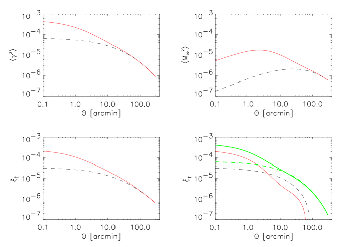
Figure 7 shows the linear and non-linear predictions for all the statistics defined here, for a particular cosmological model.

Dependence on cosmological parameters

Figure 8.: 1-$\sigma$, 2-$\sigma$ and 3-$\sigma$ confidence contours for the maximum likelihood analysis on the four parameters $\Omega_{\rm m}$, $\sigma_{8}$, $\Gamma$ and the source redshift parameter $z_{\rm s}$ (see text). The six possible pairs of parameters are displayed. On each figure, the two hidden parameters are marginalized such that $\Omega_{\rm m}\in[0.2,0.4]$, $\sigma_{8}\in[0.8,1.1]$, $\Gamma\in[0.1,0.3]$ and $z_{\rm s}\in[0.4,0.5]$, and the cosmological constant is fixed to $\Omega_{\Lambda}=1-\Omega_{\rm m}$. The reference model is $\Omega_{\rm m}=0.3$, $\sigma_{8}=1$, $\Gamma=0.21$ and $z_{\rm s}=0.44$. The survey area is $A=16\,{\rm deg}^{2}$, the galaxy ellipticity r.m.s. is $0.3$, and the correlation functions are measured in the range $0^{\prime}6<\theta<30^{\prime}$.

Figure 9.: Same as figure 8 with strong priors: in each figure, the two hidden parameters as assumed to be known perfectly. These plots show the degeneracy directions among all the possible pairs of parameters obtained from $\Omega_{\rm m}$, $\sigma_{8}$, $\Gamma$ and $z_{\rm s}$.

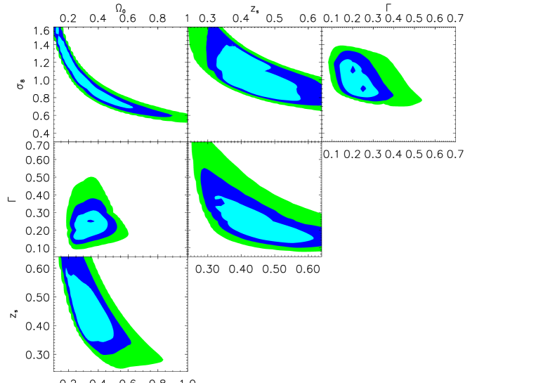
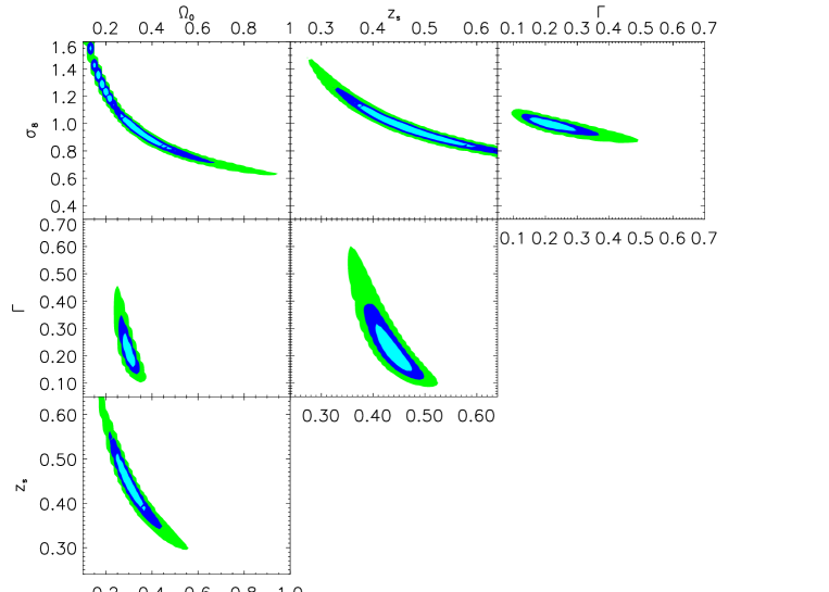
It is obvious from Eq(16), Eq(29) and Eq(30) that the cosmic shear signal depends primarily on the source redshift $w_{S}$, then on the mean density parameter $\Omega_{0}$, and on the slope and the normalization ($\sigma_{8}$) of the mass power spectrum. To explore the parameter dependence of the cosmic shear signal, we assume the Cold Dark Matter model, with a power spectrum parameterized with the slope parameter $\Gamma$. We allow the four parameters ($\Omega_{0},z_{s},\Gamma,\sigma_{8}$) to vary, and we compute the likelihood ${\cal L}(\Omega_{0},z_{s},\Gamma,\sigma_{8}\;|\;{\rm\bf d})$ of the parameters knowing the data $\bf d$. The data vector is for instance the aperture mass or any other statistic:

$${\cal L}={1\over(2\pi)^{n/2}\left|{\bf S}\right|^{1/2}}~{}\exp{\left[-{1\over 2}\left({\rm{\bf d}-{\bf s}}\right)^{T}{\bf S}^{-1}\left({\rm{\bf d}-{\bf s}}\right)\right]},$$ (48)

where ${\bf s}$ is the fiducial model vector and ${\bf S}:=\langle\left({\rm{\bf d}-{\bf s}}\right)^{T}\left({\rm{\bf d}-{\bf s}}\right)\rangle$ is the covariance matrix. Figure 8 and 9 show the parameter dependence one expects for a survey covering $16$ square degrees up to the limiting magnitude $I_{AB}=24$, for two different choices of priors. The signal also depends on other cosmological parameters ($\Omega_{b}$, $\Omega_{\Lambda}$, $\Omega_{\nu}$,…), albeit to a lower extend. For precision cosmology, all parameters are relevant, but the first constraints obtained so far from cosmic shear are on the main four parameters ($\Omega_{0},z_{s},\Gamma,\sigma_{8}$).

2.2. Galaxy ellipticities and estimators

Ellipticity of the galaxies

As mentioned in the previous Section, the cosmic shear signal is measured from the shape of the distant lensed galaxies. It is quantified from the ellipticity ${\bf e}$. The raw ellipticity ${\bf e}$ of a galaxy is measured from the second moments $I_{ij}$ of the surface brightness $f({{\hbox{$\bf\theta$}}})$:

$${\bf e}=\left({I_{11}-I_{22}\over Tr(I)};{2I_{12}\over Tr(I)}\right),\ \ \ I_{ij}=\int{\rm d}^{2}\theta W(\theta)\theta_{i}\theta_{j}f({{\hbox{$\bf\theta$}}}).$$ (49)

The window function $W({{\hbox{$\bf\theta$}}})$ suppresses the noise at large distances from the object center. The cosmic shear signal can also be measured using gravitational magnification from the relative size and number count of the lensed galaxies, but this is out of the scope of this paper. Here, we only focus on the gravitational distortion effect. If one could measure the shape of the galaxies (with $W({{\hbox{$\bf\theta$}}})=1$) perfectly without any systematics coming from the telescope tracking and the optical defects, and if the galaxies were only lensed, then the observed ellipticity would be related to the source ellipticity as

$${\bf e}^{obs}={{\bf e}^{source}+{\bf g}\over 1+{\bf e}^{source}\cdot{\bf g}},$$ (50)

where ${\bf g}={{\hbox{$\bf\gamma$}}}/(1-\kappa)$ is the reduced shear, and ${\bf e}^{obs}$ is the observed ellipticity, ${\bf e}^{source}$ is the source (unobserved) ellipticity. For nearly all cosmic shear application, the lens fields are small ($|{\bf g}|,\kappa\ll 1$) and the linear approximation is valid ${\bf e}^{obs}\simeq{\bf e}^{source}+{{\hbox{$\bf\gamma$}}}$.

Figure 10.: Right plots: simulated cores of anisotropic PSF’s. Left plots: simulated outer part of the PSF (Erben et al. 2001). The different PSFs are computed from ray-tracing through the telescope optic.

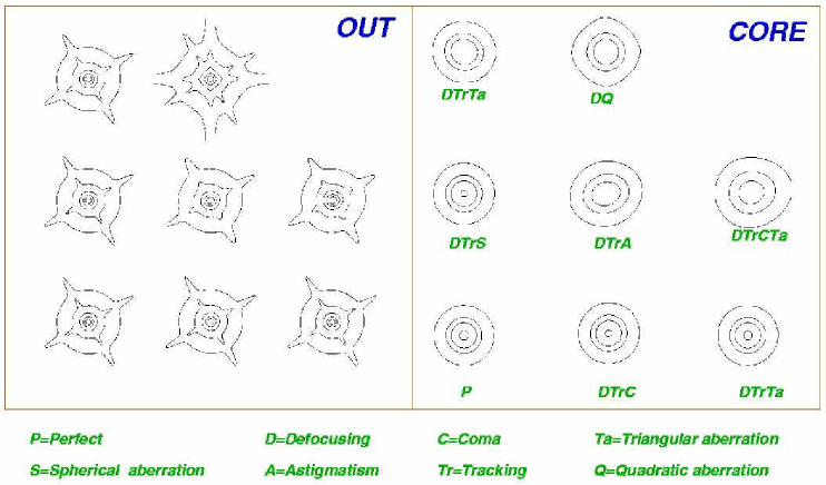
Unfortunately, the ellipticity of the galaxies measured on the images are contaminated by atmospheric and instrumental distortions of the Point Spread Function (PSF) that also produce coherent non-gravitational elongation patterns, even on stars. Such example of PSF is displayed on Figure 10, and the measured coherence of the PSF distortion on a real field is shown on Figure 11. This is a critical issue, for instance there were two early tentatives to measure the gravitational lensing by large scale structures, which failed because the image quality was very low and the PSF correction not accurate (Valdes et al. 1983, Mould et al. 1994). Since then, various methods have been developped to correct for the non gravitational source of galaxy alignment, which followed the improvement of image quality:

• Kaiser et al. (1995), a method which treats the PSF convolution analytically to the first order. It is called KSB.

• Bonnet & Mellier (1995), which combines galaxy image simulation and optimal weighting of the isophotes.

• The auto-correlation function (Van Waerbeke et al. 1997), similar to Bonnet & Mellier (1995), but applied to the auto-correlation of the image of the galaxies to avoid some problems associated with the galaxies.

• Kuijken (1999), a method which parametrizes the PSF and the galaxies with analytical functions, and try to match the convoled profile to the data.

• Kaiser (2000), extended KSB, which circularises the PSF before the isotropic correction.

• Modified KSB (Rhodes et al. 2000), is the KSB approach, applied on the galaxy moments instead of the ellipticities.

• Bernstein & Jarvis (2002), is first a circularisation of the PSF, and then the convolved profile is analysed using a reduced set of orthogonal functions (Laguerre polynomials).

• The shapelets approach (Chang & Réfrégier, 2002), is a kind of Principal Components Analysis, using orthogonal Hermite polynomials functions to decompose the convolved galaxy images (see also Bertin 2001 for a PCA approach).

The most popular, and certainly the most intensively tested (Erben et al. 2001, Bacon et al. 2001), is the KSB approach. It is a very simple and powerful correction based on the first order effect of a convolution. The idea is that we can write the first order effect of the shear and of the PSF convolution analytically as:

$${\bf e}^{obs}={\bf e}^{source}+{\rm P}_{\gamma}\cdot{{\hbox{$\bf\gamma$}}}+{\rm P}^{sm}\cdot{\bf e}^{\star},$$ (51)

where ${\rm P}_{\gamma}$ and ${\rm P}^{sm}$ are tensors computed on the image (see Kaiser et al., 1995), ${\bf e}^{\star}$ is the star ellipticity at the galaxy location, and $\bf\gamma$ is the shear signal we want to measure. Assuming that the galaxies are isotropically oriented in the source plane, we have $\langle{\bf e}^{source}\rangle=0$ (which is valid even if the galaxies are intrinsically correlated), therefore the shear estimate from the measured galaxy ellipticity is given by:

$${{\hbox{$\bf\gamma$}}}={\rm P}_{\gamma}^{-1}\left({\bf e}^{obs}-{\rm P}^{sm}\cdot{\bf e}^{\star}\right).$$ (52)

We discussed in the previous section how the shear ($\bf\gamma$) could be splitted into a radial and a tangential component $\gamma_{r}$ and $\gamma_{t}$ when projected onto the local frame of the aperture (Figure 5). Figure 12 shows the relation between the components ${\bf e}=(e_{1},e_{2})$ of a galaxy, and its orientation. If we identify $(e_{1},e_{2})$ to $(e_{t},e_{r})$, we obtain the orientation in the local frame.

Figure 11.: Uncorrected (left) and corrected(right) star ellipticities in one of cosmic shear fields.

Figure 12.: Value of ($e_{t}$,$e_{r}$), or ($e_{1}$, $e_{2}$) in Cartesian coordinates, as a function of the shape of a galaxy with respect to the local frame attached to the galaxy. Note that the ellipticity is invariant by a rotation of $\pi$, and not $2\pi$, this is why $e_{t}<0$ and $e_{r}=0$ for a vertical galaxy for instance.

E and B modes

The gravitational field is supposed to be completely dominated by a scalar gravitational potential at low redshift. The consequence is that only curl free modes for the shear are allowed. Any significant curl component should be interpreted as a (bad) sign of residual systematics in the data. Figure 13 shows the E mode generated by over-densities (top-left) and under-densities (top-right). The two bottom curl modes are not allowed.

Figure 13.: Top patterns: shear curl free modes (E modes) allowed by gravitational lensing. Bottom patterns: curl modes (B modes) not allowed from a scalar gravitational potential. Only the E modes gives the signal of the aperture mass statistics $\langle M_{\rm ap}^{2}\rangle$.

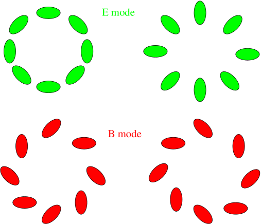
Using the statistical properties of these patterns and the ($e_{t}$,$e_{r}$) conversion from Figure 12, it can be shown that the E modes correspond to the aperture mass $\langle M_{\rm ap}^{2}\rangle$, and the B mode to the aperture mass with the galaxies $45$ degrees rotated (such rotation corresponds to a switch $e_{t}\rightarrow e_{r}$; $e_{r}\rightarrow-e_{t}$). This is easy to understand: if there is no B mode, then switching the E into B, and B into E modes kills the signal measured with the aperture mass statistics.

Aperture mass from the shear correlation function

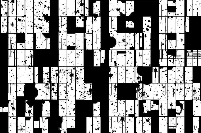
Because the E/B mode separation provides a direct and robust check of systematics error residuals, it is widely believed to be the most reliable statistics. In order to compute it, there is fortunately no need to draw a compensated filter across the data and to average the shear variance; otherwise, this could be terribly complicated with real data because of the complex shape of the masks (see Figure 14). Variances and correlation functions can be expressed one into another (since they are only linear combinaison one to another). The $E$ mode aperture mass is given by

Figure 14.: Mask area for real data. These holes of various sizes make the mass reconstruction very challenging. Each CCD chip is about $7^{\prime}\times 14^{\prime}$. Entire CCD’s had to be removed because of bright stars and residual fringes patterns.

$$\langle M_{\rm ap}^{2}\rangle=\pi\int_{0}^{2\theta_{c}}rdr{\cal W}(r)\xi_{+}(r)+\pi\int_{0}^{2\theta_{c}}rdr\tilde{\cal W}(r)\xi_{-}(r),$$ (53)

where ${\cal W}(r)$ and $\tilde{\cal W}(r)$ are given in Crittenden et al. 2002 and Pen et al. 2002. The $B$-mode is obtained by changing the sign of the second term in Eq.(53). The correlation functions $\xi_{+}(r)$ and $\xi_{-}(r)$ are compute from the tangential and radial correlation functions (see Eq.47). In order to estimate the shear correlation functions, let ${{\hbox{$\bf\theta$}}}_{i}$ be location of the $i$-th galaxy, its ellipticity ${\bf e}({{\hbox{$\bf\theta$}}}_{i})=(e_{1},e_{2})$, and the weight $w_{i}$. The ellipticity is an unbiased estimate of the shear ${{\hbox{$\bf\gamma$}}}({{\hbox{$\bf\theta$}}}_{i})$. The quantity measured from the data are the binned tangential and radial shear correlation functions. They are given by a sum over galaxy pairs $({{\hbox{$\bf\theta$}}}_{i},{{\hbox{$\bf\theta$}}}_{j})$

$$\xi_{tt}(r)={\displaystyle\sum_{i,j}w_{i}w_{j}e_{t}({{\hbox{$\bf\theta$}}}_{i})\cdot e_{t}({{\hbox{$\bf\theta$}}}_{j})\over\displaystyle\sum_{i,j}w_{i}w_{j}}\ \ \ ;\ \xi_{rr}(r)={\displaystyle\sum_{i,j}w_{i}w_{j}e_{r}({{\hbox{$\bf\theta$}}}_{i})\cdot e_{r}({{\hbox{$\bf\theta$}}}_{j})\over\displaystyle\sum_{i,j}w_{i}w_{j}},$$ (54)

where $r=|{{\hbox{$\bf\theta$}}}_{i}-{{\hbox{$\bf\theta$}}}_{j}|$, and $(e_{t},e_{r})$ are the tangential and radial ellipticities defined in the frame of the line connecting a pair of galaxies. The weights $w_{i}$ are usually computed for each galaxy from the intrinsic ellipticity variance $\sigma_{e}^{2}$ and the r.m.s. of the ellipticity PSF correction $\sigma_{\epsilon}^{2}$. For example, van Waerbeke et al (2000) measured $\sigma_{e}\simeq 0.4$ from their CFHT data, and defined the weights as:

$$w_{i}={1\over\sigma_{e}^{2}+\sigma_{\epsilon}^{2}}.$$ (55)

To compute $\sigma_{\epsilon}$ for each galaxy, the galaxy size-magnitude parameter space is divided into cells of constant object number (typically $30$ galaxies per cell). For each cell the r.m.s. of the ellipticity correction among the galaxies in the cell is computed. This choice of parameter space is motivated by the fact that the isotropic PSF correction (the $P_{\gamma}$ term in Eq.51) is mainly sensitive to the size and magnitude of the galaxies.

3. 2-pts statistics

3.1. Measurements

Figure 15.: Compilation of recent results of top-hat shear variance measurements from several groups (Courtesy Réfrégier et al. 2002).

Figure 16.: Measurement of all the 2-points statistics in the same survey, VIRMOS (Van Waerbeke et al. 2001). Top left: top-hat variance. Top right: aperture mass $E$ and $B$ modes. Bottom left: full shear correlation function. Bottom right: projected shear correlation functions. survey. Right: $E$ (top) and $B$ (bottom) modes measured in the RCS survey. The $B$ mode is low and the $E$ mode compatible with the predictions for the aperture mass statistics. The lines are fiducial models which indicate the relative deviations between the statistics to the models.

Figure 17.: Left: $E$ (top) and $B$ (bottom) modes measured with all the most recently reduced data in the VIRMOS survey (Van Waerbeke et al. 2002). Right: $E$ (top) and $B$ (bottom) modes measured in the RCS survey (Hoekstra et al. 2002). The $B$ mode is low and the $E$ mode compatible with the predictions for the aperture mass statistics.

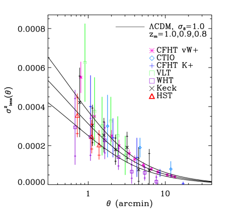
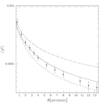
There are now several evidences of the cosmological origin of the measured signal:

(a) The consistency of the shear excess variance measured from different telescopes, at different depths and with different filters. This is summarized on Figure 15. The first detections were obtained by Bacon et al. 2000, Kaiser et al. 2000, Van Waerbeke et al. 2000, Wittman et al. 2000. Since then, several measurements have been done in different observing conditions, which are summarized in Table 1.

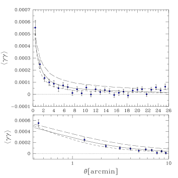
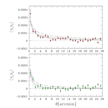
(b) On a single survey, the self consistency of the different types of lensing statistics given by Eqs.(40,42,45,47). This was done on the VIRMOS-DESCART survey , and it is shown in Figure 16 (Van Waerbeke et al. 2001).

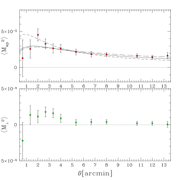
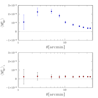
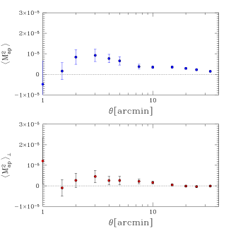
(c) The comparison of the $E$ and $B$ modes measurements (to higher accuracy than in (b)) between a deep and shallow survey for the VIRMOS-DESCART and RCS surveys (Van Waerbeke et al. 2002, Hoekstra et al. 2002). This is shown on Figure 17. More recently, the $E$ and $B$ modes have been also measured in other surveys (Brown et al. 2003, Jarvis et al. 2003, Hamana et al. 2003), which supports the cosmological origin of the signal, showing also the already small amount of residual systematics achieved with today’s technology. The $E$ and $B$ mode measurements should now be considered as the most robust proof of the cosmological origin of the signal, and a quantitative test of systematics.

(d) The lensing signal is expected to decrease for low redshift sources, as consequence of the lower efficiency of the the gravitational distortion. It corresponds to a change in $w_{s}$ in Eq(16), or equivalently a change in the mean source redshift with Eq(29). This decrease of the signal has been observed for the first time with the comparison of the $E$ mode amplitude of the VIRMOS survey aperture mass (see Figure 17), which has a source mean redshift around $0.9$, to the RCS which has a source mean redshift around $0.6$. The expected decrease in signal amplitude is about $2$, which is what is observed. This is a direct evidence of the effect of changing the redshift of the sources, a kind of 3-D cosmic shear effect.

(e) Space images provide in principle a systematics-low environment, and even if the observed areas are still smaller than ground based observations, space data provide ideal calibrations of the cosmic shear signal (Rhodes et al. 2001, Haemmerle et al. 2002, Réfrégier et al. 2002), which are in agreement with ground based measurements (see Figure 15, the HST points).

3.2. Constraints

The standard approach is to compute the likelihood of a set of $n$ parameters $(p_{1},p_{2},...,p_{n})$, knowing the data vector ${\bf d}$, as written in Eq(48). As the data vector, it is natural to choose the aperture mass variance as a function of scale $\langle M_{\rm ap}^{2}\rangle$, because the signal is splitted into gravitational lensing and systematics channels (the $E$ and $B$ modes). The $B$ mode measures an estimate of the contamination of the $E$ mode by systematics. The $E$ and $B$ modes do not equally contribute to systematic, but we know, from the measurement of the modes on the stars, that they are very similar. If the $B$ mode is not consistent with zero (which is the case for all surveys at the moment), it is important to deal with it properly when estimating the cosmological parameters. Unfortunately it is not yet clear what the best approach is: some groups (Van Waerbeke et al. 2002, Hoekstra et al. 2002, Hamana et al. 2003) added the $B$ mode in quadrature to the $E$ errors, taking into account the correlation between various scales. The $B$ mode has been subtracted first from the $E$ mode in Hoekstra et al. (2002), but not in Van Waerbeke et al. (2002). This might probably result in a slight bias for high $\sigma_{8}$ values in the later. Unfortunately we have no guarantee that the $B$ subtraction is the right correction method. Recently Jarvis et al. (2003) marginalised the probabilities over $E-B$ to $E+B$ taken as the signal, which is more likely to include the ’true’ $B$ mode correction one has to apply.

Figure 18.: Plot showing the relative amplitude of the aperture mass $E$ and $B$ modes (points without and with error bars respectively) for all the surveys where the aperture mass has been measured (Hoekstra et al. 2002, Van Waerbeke et al. 2002, Jarvis et al. 2003 and Hamana et al. 2003) (picture taken from Jarvis et al. 2003 and extended). The result of Hoekstra et al. (2002) is for the full magnitude range, while in Figure 17, right panel, it is for the galaxies used for the cosmic shear analysis.

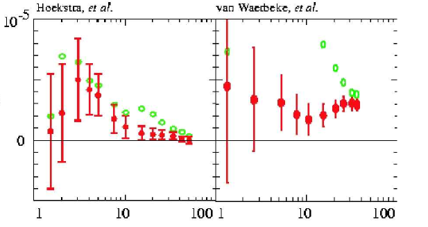
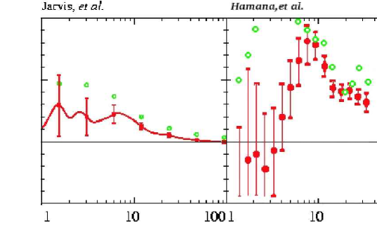
Figure 18 shows the $E$ and $B$ modes that have been measured so far, using the aperture mass only (this is the only statistic which provides an unambiguous $E$ and $B$ separation, Pen et al. 2002). The two deepest surveys have large scale $B$ mode contamination (Van Waerbeke et al. 2002, Hamana et al. 2003), and the two shallow surveys have small scale contamination (Hoekstra et al. 2002, Jarvis et al. 2003).

Figure 19.: The solid lines on each plot show the 1, 2 and 3$\sigma$ contours of the VIRMOS and RCS survey, from the measurements shown in Figure 17. The contours have been marginalised over the source redshift and the slope of the matter power spectrum as described elsewhere (Van Waerbeke et al. 2002, Hoekstra et al. 2002).

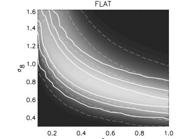
Figure 19 shows the joint $\Omega_{m}$, $\sigma_{8}$ constraints obtained from the measurements of Figure 17. They are obtained only when comparing the measured lensing signal to the non-linear predictions. Unfortunately, the actual surveys are not yet big enough to probe the linear scales accurately. The non-linear power can be computed numerically (Smith et al. 2002), but its precision is still uncertain. Recent investigations show that a $10\%$ r.m.s. uncertainty is expected, which means that the cosmological parameters cannot be known with better precision for the moment. According to the Figure 7, the transition scale between the linear and non-linear regimes is around 1 degree. The consequence is that the quoted mass normalization $\sigma_{8}$ is sensitive to the validity of the non-linear mapping at small scale. In this respect, Jarvis et al. (2003) are less contaminated by this problem because they used the lensing signal from $30^{\prime}$ to $100^{\prime}$ to constrain the mass normalization.

Table 1 summarizes the $\sigma_{8}$ measurements for all the lensing surveys published so far. For simplicity it is given for $\Omega_{m}=0.3$. Despite the differences among the surveys, it is worth to note that the results are all consistent within $2.5\sigma$ between the most extreme cases, when poorly known parameters are marginalised.

Table 1.: Constraints on the power spectrum normalization ”$\sigma_{8}$” for $\Omega_{m}=0.3$ for a flat Universe, obtained from a given ”statistic”. ”CosVar” tells us whether or not the cosmic variance has been included, ”E/B” tells us whether or not a mode decomposition has been used in the likelihood analysis. Note that Van Waerbeke et al. (2001) and Brown et al. (2003) measured a small B-mode, which they didn’t use in the parameter estimation. $z_{s}$ and $\Gamma$ are the priors used for the different surveys identified with ”ID”. Note also the cosmic shear results obtained by Kaiser et al. (2000) and Haemmerle et al. (2002), which are not in the table here because they reported a shear detection, not a $\sigma_{8}$ measurement.

ID	$\sigma_{8}$	Statistic	Field	$m_{\rm lim}$	CosVar	E/B	$z_{s}$	$\Gamma$
Maoli et al. 01	$1.03\pm 0.05$	$\langle\gamma^{2}\rangle$	VLT+CTIO	-	no	no	-	0.21
			+WHT+CFHT
Van Waerbeke et al. 01	$0.88\pm 0.11$	$\langle\gamma^{2}\rangle$, $\xi(r)$, $\langle M_{\rm ap}^{2}\rangle$	CFHT 8 sq.deg.	I=24	no	no (yes)	1.1	0.21
Rhodes et al. 01	$0.91^{+0.25}_{-0.29}$	$\xi(r)$	HST 0.05 sq.deg.	I=26	yes	no	0.9-1.1	0.25
Hoekstra et al. 02	$0.81\pm 0.08$	$\langle\gamma^{2}\rangle$	CFHT+CTIO	R=24	yes	no	0.55	0.21
			24 sq.deg.
Bacon et al. 03	$0.97\pm 0.13$	$\xi(r)$	Keck+WHT	R=25	yes	no	0.7-0.9	0.21
			1.6 sq.deg.
Réfrégier et al. 02	$0.94\pm 0.17$	$\langle\gamma^{2}\rangle$	HST 0.36 sq.deg.	I=23.5	yes	no	0.8-1.0	0.21
Van Waerbeke et al. 02	$0.94\pm 0.12$	$\langle M_{\rm ap}^{2}\rangle$	CFHT	I=24	yes	yes	0.78-1.08	0.1-0.4
			12 sq.deg.
Hoekstra et al. 02	$0.91^{+0.05}_{-0.12}$	$\langle\gamma^{2}\rangle$, $\xi(r)$	CFHT+CTIO	R=24	yes	yes	0.54-0.66	0.05-0.5
		$\langle M_{\rm ap}^{2}\rangle$	53 sq.deg.
Brown et al. 03	$0.74\pm 0.09$	$\langle\gamma^{2}\rangle$, $\xi(r)$	ESO 1.25 sq.deg.	R=25.5	yes	no (yes)	0.8-0.9	-
Hamana et al. 03	$(2\sigma)0.69^{+0.35}_{-0.25}$	$\langle M_{\rm ap}^{2}\rangle$, $\xi(r)$	Subaru 2.1 sq.deg.	R=26	yes	yes	0.8-1.4	0.1-0.4
Jarvis et al. 03	$(2\sigma)0.71^{+0.12}_{-0.16}$	$\langle\gamma^{2}\rangle$, $\xi(r)$, $\langle M_{\rm ap}^{2}\rangle$	CTIO 75 sq.deg.	R=23	yes	yes	0.66	0.15-0.5

4. 3-pts statistics

Figure 20.: Average shear pattern obtained around a galaxy pair located at (${\bf x}_{1}$, ${\bf x}_{2}$). A third galaxy is located at ${\bf x}$, its shear vector is projected along the vertical axis, it is called $\gamma_{t}({\bf x})$. The shear 3-points function $\langle{{\hbox{$\bf\gamma$}}}({\bf x}_{1})\cdot{{\hbox{$\bf\gamma$}}}({\bf x}_{2})\gamma_{t}({\bf x})\rangle$ is averaged inside the ellipse indicated by the solid line.

So far, we only discussed the 2-points statistics, but recently higher order statistics have been also developed for cosmic shear (Bernardeau et al. 1997, Jain & Seljak 1997). If we were able to reconstruct the convergence from the shear (ellipticity) measured on the galaxies, one could for instance measure the top-hat smoothed higher order statistic easily. For instance, the skewness of the convergence, which is defined as

$$S_{3}(\kappa)={\langle\kappa^{3}\rangle\over\langle\kappa^{2}\rangle^{2}},$$ (56)

is of great interest because this suited ratio of moments makes this statistic nearly independent of the normalization and shape of the power spectrum (Bernardeau et al. 1997). A pedagogical way to compare the second and third moments is to compute $\langle\kappa^{2}\rangle$ and $S_{3}(\kappa)$ in the perturbation theory, and with a power law power spectrum. In that case, one finds

$$\sigma_{\kappa} \approx 0.01\ \sigma_{8}\ \Omega_{0}^{0.8}\ \left({\theta_{0}\over 1{\rm deg.}}\right)^{-(n+2)/2}\ z_{s}^{0.75},$$ (57)

$$s_{3} \sim {\langle\kappa^{3}\rangle\over\langle\kappa^{2}\rangle^{2}}\approx 40\ \Omega_{0}^{-0.8}\ z_{s}^{-1.35}.$$ (58)

These are only approximated relations, which are not valid in the real (non-linear) world, but it shows that the skewness provides a direct geometrical test (dependence on $\Omega_{0}$), as long as we know the redshift of the sources $z_{s}$. Combined with the second order moment, the degeneracy between the power spectrum normalization and the density parameter can be broken with the cosmic shear alone.

The skewness can also be predicted in the non-linear regime, as for the 2-points statistics, using a non-linear extension of the bispectrum (Scoccimarro et al. 2002, Van Waerbeke et al. 2002). The problem with the skewness of the convergence is that it cannot be measured on the data directly, and one needs to reconstruct $\kappa$ from the shear first. This process is unfortunately sensitive to the survey geometry because the projected mass reconstruction is essentially a non-linear process. Given the typical observed field geometry, as shown on Figure 14, it is yet impossible to perform a mass reconstruction with the accuracy required to measure the cosmic shear effect. One possibility for avoiding the mass reconstruction (that is try to make the map making a local process) is to compute the third moment of the aperture mass (Schneider et al. 1998). Unfortunately, in that case as well, the complicated survey geometry make it difficult to measure an accurate third moment $\langle M_{\rm ap}^{3}\rangle$.

The alternative is to measure a third moment on the shear field itself, but this cannot be done in a trivial way, since for evident symmetry reasons, any odd moment of the components of a vector field vanishes. One has to built explicitly non-trivial measures of the third moment of the shear, which has been recently proposed. So far, two of the proposed estimators lead to a measurement (Bernardeau et al. 2002 and Pen et al. 2002).

In Bernardeau et al. (2002) the idea is to identify regular shear patterns around any pair of lensed galaxies. A pair is identified by the two galaxy positions ${\bf x}_{1}$ and ${\bf x}_{2}$, and any location around the pair by ${\bf x}$. For a fixed pair (${\bf x}_{1}$, ${\bf x}_{2}$), we are interested in the average shear at ${\bf x}$.

Figure 20 shows the typical shear pattern observed around a galaxy pair located at (${\bf x}_{1}$, ${\bf x}_{2}$). Ray tracing simulations demonstrate the stability of this shear pattern, which is almost independent on the cosmological model and the pair separation. A natural 3-points function to calculate is the average of the product of the shear correlation function ${{\hbox{$\bf\gamma$}}}({\bf x}_{1})\cdot{{\hbox{$\bf\gamma$}}}({\bf x}_{2})$ with a projection of the shear of the third galaxy $\gamma({\bf x})$. It is obvious from Figure 20 that the projection is optimal when performed along the vertical axis. For a fixed pair location (${\bf x}_{1}$, ${\bf x}_{2}$), the 3-points function $\xi_{3}({\bf x})$ is defined as:

$$\xi_{3}({\bf x})=\langle{{\hbox{$\bf\gamma$}}}({\bf x}_{1})\cdot{{\hbox{$\bf\gamma$}}}({\bf x}_{2})\gamma_{t}({\bf x})\rangle,$$ (59)

and the quantity we measure is:

$$\overline{\xi_{3}}(|{\bf x}_{1}-{\bf x}_{2}|)=\int_{\rm Ell.}{{\rm d}^{2}{\bf x}^{\prime}\over V_{\rm Ell.}}\xi_{3}({\bf x}^{\prime}).$$ (60)

Figure 21.: On the left, results for $\overline{\xi_{3}}(d_{12})/\overline{\xi_{2}}(d_{12})^{2}$ for the VIRMOS-DESCART survey (dot-dashed lines: $E-B$ mode for the 2-points function, solid line: $E+B$ mode for the 2-points function). This is compared to $\tau$CDM and OCDM results (dotted and dashed lines respectively). Right plot: dashed line is $\overline{\xi_{3}}(d_{12})$ for the VIRMOS-DESCART survey, compared to the same quantity measured on the stars.

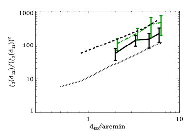
Figure 21 shows the result on the VIRMOS-DESCART survey. The treatment of the $B$ mode is still uncertain, and the redshift uncertainty still too large, which makes very difficult the interpretation in terms of cosmological parameters. However Figure 21 shows that the order of magnitude, and the slope of the signal are consistent with the expectations. For instance, the signal from the stars before PSF correction is completely different in shape and amplitude.

Figure 22.: Skewness of the convergence as measured in Pen et al. (2002), on the VIRMOS-DESCART survey. The overall significance of the measurement if $3.3\;\sigma$, which was computed using Monte Carlo sampling of the errors from ray-tracing simulations. A comparison of the signal with tese simulations shows that $\Omega_{0}<0.4$ at the $90\%$ level.

In Pen et al. (2002), the idea is to compute the convergence aperture mass 3-points function from an integral of the shear 3-points function. This solution avoids the problem of drawing cells across a complex field geometry and presents the advantage to estimate the third moment of the convergence $\kappa$, which is the field of physical interest. Unfortunately, its measurement is still very noisy, because it uses a compensated filter that removes the low frequency modes for any target frequency (which is not the case for a top-hat filtering). The resulting skewness is shown on Figure 22, and is consistent with $\Omega_{0}<0.4$ at the $90\%$ level.

Other approaches have been proposed (Zaldarriaga & Scoccimarro 2002, Schneider & Lombardi 2003, Takada & Jain 2003) which all deal with trying to optimize the signal-to-noise by looking for the best galaxies triangle configurations containing the highest signal. They have not yet been applied to the data.

5. Galaxy biasing

A direct byproduct of cosmic shear observations is the measure of the light/mass relation, the so-called biasing parameter $b$ defined as the ratio of the galaxy density contrast to the dark matter density contrast

$$\delta_{\rm gal}=b\;\delta_{\rm mass}.$$ (61)

This is in fact a highly simplified model, which assumes that the biasing does not vary with scale and redshift, and that the relation between mass and light is deterministic. While in the real world, none of these assumptions are correct, this model has the advantage to be tractable analytically, and to provide an average biasing estimates, which is still very useful. Nevertheless, it is possible to go beyond this simple model by combining a measurement of the dark matter clustering, galaxy clustering, and their cross-correlation by defining a biasing $b$ and cross-correlation $r$ such that:

$$b={\langle N_{\rm ap}^{2}\rangle\over\langle M_{\rm ap}^{2}\rangle};\;\;r={\langle M_{\rm ap}N_{\rm ap}\rangle\over\langle N_{\rm ap}^{2}\rangle^{1/2}\langle M_{\rm ap}^{2}\rangle^{1/2}},$$ (62)

Figure 23.: Left plot: The measurements of $\langle{\cal N}^{2}\rangle$ (panel a), and $\langle{\cal N}M_{\rm ap}\rangle$ (panel b) as a function of angular scale from the RCS data. Panel c shows $\langle M_{\rm ap}^{2}\rangle$ as a function of angular scale from the VIRMOS-DESCART data. The error bars for $\langle M_{\rm ap}^{2}\rangle$ have been increased to account for the unknown correction for the observed “B”-mode. For reference, a few models have been plotted, assuming $b=1$ and $r=1$, for an OCDM cosmology (dotted line; $\Omega_{m}=0.3$, $\Omega_{\Lambda}=0$, $\sigma_{8}=0.9$, and $\Gamma=0.21$) and a $\Lambda$CDM cosmology (dashed line; $\Omega_{m}=0.3$, $\Omega_{\Lambda}=0.7$, $\sigma_{8}=0.9$, and $\Gamma=0.21$). Note that the points at different scales are only slightly correlated. Right plot: The measured value of the galaxy-mass cross correlation coefficient $r$ as a function of scale for the $\Lambda$CDM cosmology. (b) The bias parameter $b$ as a function of scale. The upper axis indicates the effective physical scale probed by the compensated filter at the median redshift of the lenses $(z=0.35)$.

where $N_{\rm ap}$ is the galaxy number count density contrast smoothed with a compensated filter. Therefore, $N_{\rm ap}$ is similar to $M_{\rm ap}$, except that it applies to the number count instead to the shear. As we discussed before, the compensated filter is a passband filter, quite narrow in Fourier space. If one chooses the number count fluctuations $N_{\rm ap}$ to be a foreground galaxy population with a narrow redshift distribution, then the biasing and cross-correlation $b$ and $r$ emerging from Eq(62) will be relatively localized in redshift AND wavelength. The combinaison of well localized redshift and wavelength corresponds to a roughly fixed physical distance. Therefore we can say that, even with the simple scheme of galaxy biasing given by Eq(61), an estimate of $b$ and $r$ from Eq(62) is fairly local in physical scale, for the foreground galaxy population under consideration (Schneider 1998, Van Waerbeke 1998). This result has been proved to be robust against a wide range of cosmological parameters and power spectra (Van Waerbeke 1998).

This idea has been applied for the first time in the RCS data (Hoekstra et al. 2001). Unfortunately, this survey is not deep enough to provide an accurate measure of the dark matter clustering that could allow to separate $b$ and $r$. Instead, the authors measured the ratio $b/r=1.05^{+0.12}_{-0.10}$ for the favored $\Lambda$CDM model ($\Omega_{0}=0.3$ and $\Omega_{\Lambda}=0.7$). On the other hand, a combination of deep and shallow survey could help to measure the bias and the cross-correlation independently. This was done by combining the RCS and VIRMOS-DESCART surveys (Hoekstra et al., 2002). RCS is a wide shallow survey with a mean source redshift of $\sim 0.6$, and VIRMOS-DESCART is a deep survey with a mean source redshift $\sim 0.9$. By selecting the foreground population with a median redshift $\sim 0.35$ on the RCS survey, the number counts $\langle N_{\rm ap}^{2}\rangle$, and the cross-correlation $\langle M_{\rm ap}N_{\rm ap}\rangle$ were measured. The aperture mass $\langle M_{\rm ap}^{2}\rangle$ is measured on the deep survey. Figure 23 shows the measured $b$ and $r$ as a function of scale (angular scales are also converted to physical scale for a given cosmological model, with the lenses at $z=0.35$). Although a proper interpretation of the measurement requires a better knowledge of the redshift distribution and cosmological parameters, it is a direct indication of the stochasticity ($r<1$) of the biasing at small scale, and that the biasing varies with scale as we approach the galactic scales, below $1^{\prime}$. The foreground galaxies were selected in $R$, and it was found that $b=0.71^{+0.06}_{-0.04}$ on a scale $1-2\;h^{-1}_{50}\;{\rm Mpc}$, and $r$ reaches a miminum value of $r=0.57^{+0.08}_{-0.07}$, at $1\;h^{-1}_{50}\;{\rm Mpc}$. We should note that $b$ tends toward $1$ at larger scale.

6. Dark matter power spectrum inversion

The central interest in cosmic shear observation is dark matter. This is probably even more important than measuring the cosmological parameters, for which we have some hope to measure them very accurately in the future (although there is the issue of degeneracies where lensing can help). One important question is then: what can we say about the dark matter distribution, provided we know all the cosmological parameters? This is nothing else but to try to map the dark matter in the same way we map the galaxies or the cosmic microwave background, or at least to measure its power spectrum in three dimensions, for all possible scales, independently of any evolution model. This is in principle possible from a direct inversion of Eq(29), but there are two issues here. One is that virtually, all physical wavelengths $k$ are projected out to give a single angular wavelength $s$, and with a naive deprojection, one needs some cut-off somewhere in $k$-space to perform the invertion. The other issue is that the 3D power spectrum evolves non-linearly with redshift in the non-linear scales, therefore how could we be independent of any modeling when inverting the 2D convergence power? The first 2D convergence power spectrum estimate was performed in Pen et al. (2002) on the VIRMOS-DESCART data, and in Brown et al. (2003) on the COMBO-17 data, but the spectrum inversion was not done.

Figure 24.: Top: Dark matter 3D power spectrum, deprojected from the 2D convergence power spectrum measured in the VIRMOS survey, using SVD (Pen et al. 2003). The power is rescaled to $z=0$, points are compared to the CMB (WMAP) and RCS lens survey. Bottom: Galaxy 3D power spectrum deprojected using the same method. For comparison, points from 2MASS, APM and SDSS are also shown.

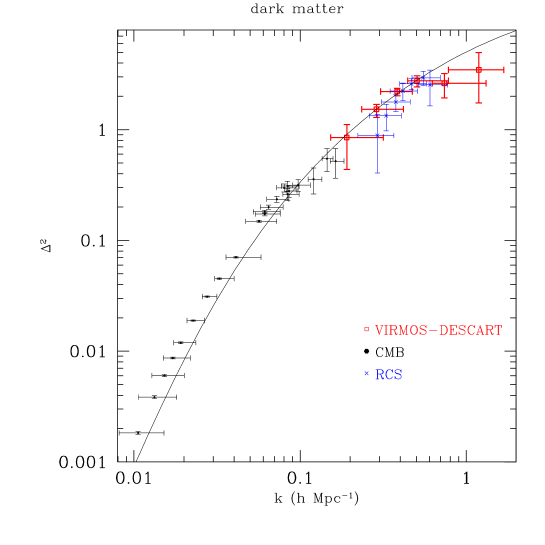
Pen et al. (2003) investigated the inversion using a singular decomposition technique, an extension of the minimum variance estimator deprojection developped in Seljak (1998). The non-linear evolution of the 3-D power spectrum was assumed to evolve linearly with redshift even in the non-linear regime. This hypothesis is, surprisingly, a viable assumption within the scale range of interest, and produces errors still smaller than the statistical errors. The result is shown on Figure 24 for the dark matter (top) and the galaxies (bottom). It shows a very nice agreement with the cosmic microwave background $C_{l}$’s (WMAP points extrapolated at $z=0$, see Spergel et al. 2003), and with clustering measurements from other galaxy surveys.

A dark matter-galaxy cross-correlation was also deprojected, allowing Pen et al. (2003) to estimate the 3D biasing $b$ and matter-light correlation $r$. They found $b=1.33\pm 0.19$ and $r=0.68\pm 0.24$ for the $I$-selected galaxies. The bias value is slightly different than the one measured from the aperture mass on the RCS survey (section 5), but we should keep in mind that the galaxy populations are different ($R$ compared to $I$ selected galaxies for the RCS and VIRMOS surveys respectively). The physical scales probed in VIRMOS are also larger because it is a deeper survey than in RCS.

Figure 25.: The two dimensional, marginalized likelihoods for the $(\Omega_{m},\sigma_{8})$ plane. The overlaid, filled contours show the 68% and 95% integration levels for the distributions. Bottom – RCS only, Middle – CMB only, Top – CMB+RCS. Courtesy Contaldi et al. 2003.

7. Gravitational Lensing and Cosmic Microwave Background

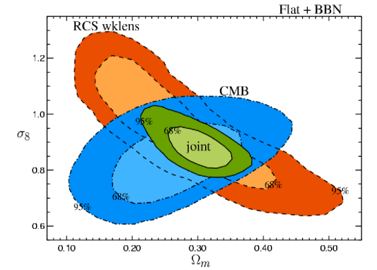
The use of lensing with other experiments improves the accuracy of cosmological parameter measurements and eventually breaks some intrinsic degeneracies attached to each. The potential interest of combining lensing by large scale structures and cosmic microwave background experiments has been studied in Hu & Tegmark (1999). The joint study of the weak lensing RCS survey and the WMAP data performed in Contaldi et al. (2003) is shown on Figure 25 and illustrates the gain of this combination: it provides a direct evidence of the low value of the matter density $\Omega_{0}$, which indicates a high non-zero value for the cosmological constant, independently of the supernovae result.

8. Approximations and Limitations

Born approximation and lens-lens coupling

The lensing theory developed in Section 1 assumes the lens can be projected onto a single plane, and therefore that the ray-tracing through a thick lens is equivalent to a thin lens appropriately weighted. As it has been quantified by Bernardeau et al. (1997), Schneider et al. (1998) or Van Waerbeke et al. (2002), it turns out to be a very good approximation. If we call $\bf\theta$ the direction of the unperturbed ray trajectory, a ray-light passing through a first lens will be slightly deflected by an angle $\bf\delta$$\bf\theta$, and will impact the second lens at a position angle ${{\hbox{$\bf\theta$}}}+{{\hbox{$\bf\delta$}}}{{\hbox{$\bf\theta$}}}$ instead of $\bf\theta$ if the light ray were unperturbed. From a perturbative point of view, it means that expression Eq(13) has a correction term because the position angle to compute the lens strength is no longer ${\bf x}=f_{K}(w){{\hbox{$\bf\theta$}}}$, but

$$x_{i}=f_{K}(w)\theta_{i}-{2\over c^{2}}\int_{0}^{w}{\rm d}w^{\prime}\;f_{K}(w-w^{\prime})\,\partial_{i}\Phi^{(1)}(f_{K}(w){{\hbox{$\bf\theta$}}},w^{\prime}).$$ (63)

Eq(13) is therefore replaced by ${\cal A}_{ij}({{\hbox{$\bf\theta$}}})=\delta_{ij}+{\cal A}^{(1)}_{ij}({{\hbox{$\bf\theta$}}})+{\cal A}^{(2)}_{ij}({{\hbox{$\bf\theta$}}})$ with

$${\cal A}_{ij}^{(2)}({{\hbox{$\bf\theta$}}},w) = -{2\over c^{2}}\int_{0}^{w}{\rm d}w^{\prime}\;{f_{K}(w-w^{\prime})f_{K}(w^{\prime})\over f_{K}(w)}$$ (64)

$$\times \left[\Phi_{,ikl}(f_{K}(w^{\prime}){{\hbox{$\bf\theta$}}},w^{\prime})\,x_{l}^{(1)}({{\hbox{$\bf\theta$}}},w^{\prime})\delta_{kj}+\Phi_{,ik}(f_{K}(w^{\prime}){\hbox{$\bf\theta$}},w^{\prime}){\cal A}_{kl}^{(1)}({{\hbox{$\bf\theta$}}},w^{\prime})\right].$$ (65)

Given that the correction to the light trajectory is a second order effect in the perturbation, it is expected to become important in any high order statistics of the lensing fields. Mathematically, indeed, they have the same order than the second order dynamical correction (which is proportional to the second order gravitational potential $\Phi^{(2)}$). It turns out that the light trajectory correction is much smaller than the dynamical second order correction. The reason is that Eq(LABEL:born) involves a second lensing efficiency factor (the ratio of angular diameter distances $f_{K}$’s), which is not present in the second order dynamical correction.

Figure 26.: Left panel: variance and skewness of the top-hat smoothed convergence field a OCDM ($\Omega_{0}=0.3$, $\sigma_{8}=0.85$, $z_{s}=1.03$, $\Gamma=0.21$) and SCDM model ($\Omega_{0}=1.$, $\sigma_{8}=0.6$, $z_{s}=1.03$, $\Gamma=0.5$). The solid lines show the non-linear predictions, and the dashed lines the leading order of the perturbation theory calculations. The vertical dotted lines in the left panels denote the reliable scale limit fixed by the resolution of the ray-tracing simulation. The “large” error bars correspond to a survey of $25$ square degrees, and the small error bars to $1000$ square degrees. Right panel: Skewness correction due to the Born approximation and lens-lens coupling for SCDM (top) and OCDM1 (bottom) measured in ray-tracing simulation.

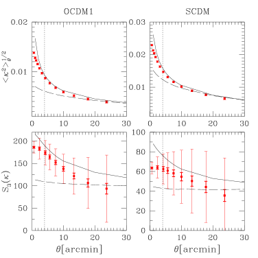
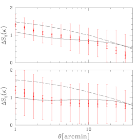
Figure 26 shows several comparisons of the non-linear prediction for the second and third order statistics with a measurement of the same statistics done in ray-tracing simulations. It clearly demonstrates that non-linear calculations give quite accurate results, and that approximations related to the ray trajectories are valid to better than $2\%$.

Non-linear lensing effects

To first approximation, we consider the galaxy ellipticity an unbiased estimate of the shear. However, Eq(50) tells us that lensing is really non-linear. This approximation has been estimated in Barber (2002): it is negligible for sources at redshift less than $z\simeq 1$ and for scales larger than $5^{\prime}$, while at smaller scale, a few percents effects could be detected. Fortunately, the use of the full non-linear lensing equation does not present any theoretical or technical difficulties, so small scale non linear lensing effect can be easily handled. It is just usually ignored in most of the theoretical and numerical works.

Non-linear modeling

On the other hand, Figure 26 also demonstrates that the accuracy of non-linear predictions on the 2-points statistics is never better better than $10\%$, while it is never better than $\sim 20-30\%$ for the skewness. This theoretical limit is a severe issue (Van Waerbeke et al. 2002) since one cannot expect to do precision cosmology if the accuracy of the model we use to extract the cosmological parameters is worse than the precision we want to reach on the cosmological parameters (that is a few percents). Smith et al. (2003) proposed an improved version of non-linear modeling, which is unfortunately still insufficient. In particular, to increase the precision, we still do not know whether the baryons have to be taken into account in the modeling or not. The goal here is a modeling accurate to $1-3\%$, if one wants to reach the same accuracy on the cosmological parameters.

Intrinsic alignment

Gravitational lensing is not the only natural process which produces alignment of galaxies over large distances. Intrinsic alignment might occur from tidal fields, and produce galaxy shape correlations over cosmological distances, and contaminate cosmological signal (Croft & Metzler 2001, Catelan & Porciani 2001, Heavens et al. 2000, Catelan et al. 2001, Hatton & Ninin 2001) which should in principle split, in a predictable way, into $E$ and $B$ modes. There is unfortunately only partial agreement between the different predictions. Moreover, most of the predictions stand for dark matter halos, while we are in fact observing galaxies, which should experience some alignment mixing. This has not been simulated so far. Concerning the dark matter halos alignment, despite the disagreement among the predictions, it is generally not believed to be higher than a $10\%$ contamination for a lensing survey with a mean source redshift at $z_{s}=1$. An exception is Jing (2002), who suggested that intrinsic alignment could dominate the cosmic shear even in deep surveys. This possibility is already ruled out by observations: this would indeed imply a very low $\sigma_{8}\sim 0.1$ if the observed signal were dominated by intrinsic alignment, and we should also observe an increase of the effect as we go from deep to shallow survey, which is not the case (see Figure 17). In any case, intrinsic alignment contamination might be an issue for studies using a single source redshift in their analysis. In the future, this will not be the case since photometric redshifts will be available. In that case, the effect can be suppressed by measuring the cosmic shear correlation between distant redshift sources, instead of measuring the fully projected signal. Consequently, intrinsic alignment should not be considered as a critical issue (Heymans & Heavens 2003, King & Schneider 2003). Pen et al. (2000) and Brown et al. (2002) reported the first two evidences for intrinsic alignment in the nearby Universe, which are not too inconsistent with the predictions.

Source clustering

Source clustering arises because a subset of sources overlap with a subset of the lenses which are probed. There is therefore a natural bias to measure the signal preferentially in high density regions, across the overlap area. This effect gives rise to correction terms in high order statistics (Bernardeau 1998). It is easy to understand the problem if we model the source redshift distribution including a clustering term:

$$p_{w}({{\hbox{$\bf\theta$}}},w)={\bar{p}}_{w}(w)(1+\delta_{gal}(f_{K}(w){{\hbox{$\bf\theta$}}},w)+...),$$ (67)

which replace the source redshift distribution $p_{w}(w)$ in Eq(18). It is then easy to see that a density coupling occurs in Eq(17). The source clustering effect was extensively studied by Hamana et al. (2002). They confirmed that it is not an issue for the 2-points statistics, but could be as high as $10-20\%$ for the skewness of the convergence, for a narrow redshift distribution. In case of the broad redshift distribution, the effect is diluted by the bulk of non-overlapping areas. For future surveys, an accurate measure of the high order statistics will require a precise estimation of this effect, which is not a problem by itself, but it must be done. Schneider et al. (2003) predicted that source clustering could produce $B$ mode in the shear maps, which has not being tested against reay-tracing simulation yet. However, the predicted amplitude is 2 orders of magnitude and below for aperture mass scales larger than $1^{\prime}$.

PSF correction

With the non-linear modeling of the power at small scale, this is certainly the most serious issue concerning the cosmological interpretation of the cosmic shear signal. Again, if we want to reach a few percents accuracy on cosmological parameters measurements, we need a PSF correction with that accuracy. So far we are able to reach $10\%$ precision with the KSB method for a typical signal measured on sources at $z=1$ (Erben et al. 2001, Bacon et al. 2001, Van Waerbeke et al. 2002). This is reasonably good, but we still need to gain one order of magnitude (in addition to the order of magnitude we need to gain for the non-linear modeling as well). The $10\%$ uncertainty is an upper limit, which comes from the large $B$ mode found in all surveys, at different scales, for probably different reasons (for instance, RCS have $B$ mode at small scale only they may have measured intrinsic alignment). This upper limit is reduced if one uses the scales with very small or no $B$ mode, but then some cosmological information is lost. So far, our understanding of the PSF modeling is insufficient in particular concerning the PSF variation (and stability) accros the CCD’s and the contribution of high frequency modes. Space data are often viewed as potentially systematics-free. This is unfortunately not true, since all space data which have been processed for cosmic shear, required a significant PSF correction. However, the main difference between space and ground based data is that, in space, the PSF is certainly more stable between exposures. But one should not forget that in space, the PSF is $100\%$ instrumental (it is the Airy spot, which is larger than the Airy spot on the ground because space telescopes are smaller), and not atmospheric at all (which it is with ground based data with larger telescopes). Dealing with a non circular Airy spot to correct for the galaxy shapes was not trivial for the Hubble Space Telescope for instance, mainly because of the severe undersampling of the PSF (Hoekstra et al. 1998). There is no intensive simulation of shear measurement under various realistic space image conditions, only qualitative estimations have been done (Réfrégier et al. 2003, Massey et al. 2003), which seems promising.

Finally, one should emphasize that the most difficult part of the PSF correction is not the anisotropic correction, which is done quite accurately, but the isotropic correction (Erben et al. 2001, Hirata & Seljak 2003). The ultimate limit of PSF correction in space and on the ground is still an open question.

9. Prospects

Figure 27.: Top hat variance of shear as function of angular scale from 6 cosmic shear surveys. The open black stars are the predictions for the CFHT-LS which will start by 2003 with Megacam at CFHT. This is the expected signal from the “Wide Survey” which will cover 170 deg² up to $I_{AB}=24.5$. For most points the errors are smaller than the stars.

Figure 28.: Theoretical expectations on cosmological models beyond the standard model from the wide CFHT Legacy Survey that will cover 170 deg². The dots with error bars are the expected measurements of cosmic shear CFHTLS data. The lines shows various models discussed by Benabed & Bernardeau (2001).

In the WMAP (Spergel et al. 2003) context, one can wonder whether future cosmic shear surveys can still provide useful cosmological informations that would not be available otherwise from CMB and SNIa experiments. The answer is clearly yes because cosmic shear is the only way to directly probe dark matter on scales that cannot be directly probed by other techniques. It can explore the properties of the dark matter together with luminous matter on quasi-linear and non-linear scales where the complexity of physical processes make theoretical and numerical predictions among the most challenging tasks for the next decade. Further, because cosmic shear is sensitive to the growth rate of perturbations integrated along the line-of-sight, the additional redshift information provides a tool to study the structure formation mechanism and the clustering history with look-back time. It is the purpose of tomography to study the 3D matter distribution by combining the lensing effect with the redshift information of the sources (Hu 1999, Heavens 2003). This clearly belongs to the prospective part, and was not discussed in the review.

The future key scientific goals are therefore the reconstruction of the 3-dimension dark matter power spectrum as function of redshift, the analysis of the properties of the relation between light and mass, and the study of the dark energy equation of state. As shown in this review, the scientific studies of the cosmic shear surveys done so far already show that there are neither conceptual nor technical barriers that hamper these goals to be achieved quickly. Tegmark & Zaldariaga (2002) with the RCS cosmic shear survey and Pen et al. (2003) with the VIRMOS-DESCART cosmic shear surveys have demonstrated that the 3-D power spectrum of the dark matter can be reconstructed. Remarkably, their results extend monotonically toward small scales the dark matter power spectrum derived from CMB experiments. Likewise, Hoekstra et al. (2001) Hoekstra et al. (2002), and Pen et al. (2003), have shown that the properties of the biasing and the dark matter-galaxy cross correlation can already be analyzed with present-day surveys. Finally, Bernardeau et al. (2003) as well as Pen et al. (2003) have shown that high order statistics are already measurable from ground based data covering 10 deg², thus providing independent informations on cosmological models, with eventually some important degeneracies broken.

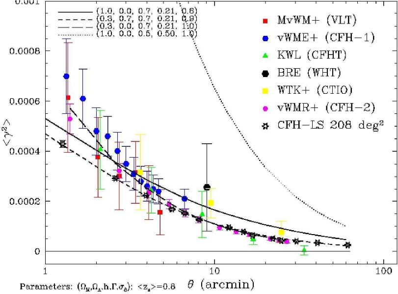
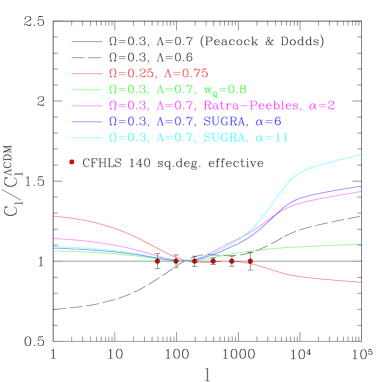
Although the B-mode contamination is still an important technical issue that may slow down the cosmic shear developments, in principle the next large, deep and multi-color surveys will be in position to address questions relevant for cosmology and fundamental physics with a high degree of precision. Such surveys, covering hundreds of degrees, with multi-bands data are about to start. Among those, the wide CFHT Legacy Survey will cover 170 deg², spread over three uncorrelated fields, in 5 optical bands, and a fraction will be followed up later in J and K bands with the wide field infrared camera WIRCAM at CFHT. Figures 27 and 28 show some predictions of CFHTLS. On Figure 27 we simulated the expected signal to noise of the shear variance as function of angular scale for a $\Lambda$CDM cosmology. The error bars are much smaller than the VIRMOS-DESCART survey which has the same depth as CFHTLS. On Figure 28, we compare the expectations of the CFHT Legacy Survey angular power spectrum with the predictions of several theoretical quintessence fields models. It shows that 200 deg² deep survey with multi-color informations to get redshift of sources, one can already interpret cosmological data beyond standard interpretations. The CFHTLS will be of considerable interest because one of the fields is also a target for the VMOS/VDDS spectroscopic survey (Le Fèvre et al 2003), the XMM-LSS survey (Pierre et al 2001) and also the COSMOS Treasury Survey that will be done by the HST/ACS instrument. Hence, in addition to a complete description of the redshift distribution of the CFHTLS galaxies, as well as of the X-ray clusters and active galaxies, high accuracy shape measurement of galaxies will be feasible. This HST/ACS data set attached to a subsample of CFHTLS data will permit to check the reliability of ground based PSF corrected shear catalogs but also to extend the shear analysis on very small scales, down to the galactic dark halos scales. Join together with CMB, we then expect to get by 2005 a complete view of the dark matter power spectrum and the biasing from Gigaparsecs down to kiloparsecs scales, as well as a detailed description of individual dark halo properties and of the redshift distribution of lenses and sources (Cooray & Sheth, 2002). One should mention the extensive search for dark matter halos in the Suprime-Cam fields (Miyazaki et al. 2003): this is more a cluster physics-oriented, but it illustrates very well the future developments with cosmic shear data for understanding the halo distribution and formation.

CFHTLS is one of the new generation surveys, with similar studies begining at SUBARU, soon at ESO, with the VST, later with VISTA, also the NOAO deep survey , Dark Matter Telescope , and the PAN-STARRS . Beyond 2005, space based dark energy/matter probes like SNAP appear as a kind of final achievement. In principle, SNAP can provide deep images, accurate photometric redshift, a large field of view and outstanding image quality one expect for cosmic shear. A dark matter space telescope, entirely dedicated to cosmic shear observations, might also be an interesting option: it could be a ’small’ telescope (therefore fairly cheap) that could observe the shear over all the sky. One could then ’see’ the dark matter everywhere!

Cosmic shear data are optimized when they are used together with other surveys, like Boomerang, CBI, DASI, WMAP of Planck CMB experiments, SNIa surveys, or galaxy surveys (2dF, SDSS). The first tentative recently done by Contaldi, Hoekstra & Lewis (2003) shows that tight constraints can really be expected in the future. Likewise, by using cosmic magnification instead of cosmic shear on the 100, 000 SDSS quasars, Ménard & Bartelmann (2002) have shown the cross-correlations between the foreground galaxy distribution and the quasar sample is also useful to explore the properties of the biasing. In principle magnification bias in the SDSS quasar sample can provide similar constrains as cosmic shear. Yet, this is a widely unexplored road.

This review shows that the Aussois winter school has been organized at a key period, between the first and second generations of cosmic shear surveys. The first period, from 1999 to 2003, demonstrated cosmic shear can be detected and exploited for a lot of cosmological questions. We now enter the next generation surveys, which will end around 2010. These are large ground based surveys (like the CFHTLS-weak lensing) which will fully exploit the new windows opened by the first surveys. Then we will enter the third (last?) period with extensive space observations, probably after 2010, like SNAP, which will permit to do precision cosmology, and maybe to close the subject.

Acknowledgments.

We are grateful to David Valls-Gabaud and Jean Paul Kneib, who organised a very exciting lensing school that closes the activivites of the LENSNET network. We would like to thank Matthias Bartelmann, Karim Benabed, Emmanuel Bertin, Francis Bernardeau, David Bacon, Dick Bond, Carlo Contaldi, Takashi Hamana, Henk Hoekstra, Bhuvnesh Jain, Brice Ménard, Ue-Li Pen, Dmitri Pogosyan, Simon Prunet, Alexandre Réfrégier, Peter Schneider and Ismael Tereno for regular stimulating discussions. This work was supported by the TMR Network “Gravitational Lensing: New Constraints on Cosmology and the Distribution of Dark Matter” (LENSNET) of the EC under contract No. ERBFMRX-CT97-0172.

References

Bacon, D., Massey, R., Réfrégier, A., Ellis, R., 2003, Joint cosmic shear Measurements with the Keck and William Herschel telescopes, astro-ph/0203134

Bacon, D.J., Réfrégier, A.R., Clowe, D., Ellis, R.S., 2001, Numerical simulations of weak lensing measurements, MNRAS, 325, 1065

Bacon, D.J., Réfrégier, A.R., Ellis, R.S., 2000, Detection of weak gravitational lensing by large-scale structure, MNRAS, 318, 625

Barber, A., 2002, The redshift and scale dependence of the cosmic shear signal from numerical simulations, MNRAS, 335, 909

Bartelmann, M., Schneider, P., 1999, Power spectrum from weak-shear data, A&A, 345, 17

Benabed, K., Bernardeau, F., 2001, Testing quintessence models with large-scale structure growth, Phys. Rev. D, 64, 3501

Bernardeau, F., 1998, The effects of source clustering on weak lensing statistics, A&A, 338, 375

Bernardeau, F., Mellier, Y., Van Waerbeke, L., 2002, Detection of non-Gaussian signatures in the VIRMOS-DESCART lensing survey, A&A, 389, L28

Bernardeau, F., Van Waerbeke, L., Mellier, Y., 1997, Weak lensing statistics as a probe of $\Omega$ and power spectrum., A&A, 322, 1

Bernstein, G., & Jarvis, M., 2002, Shapes and shears, stars and smears: optimal measurements for weak lensing, AJ, 123, 583

Bertin, E., 2001, Mining pixels: The extraction and classification of astronomical sources, in Mining the Sky, Proceedings of the MPA/ESO/MPE Workshop, Garching, 31 July-4 August, 2000. Edited by A. J. Banday, S. Zaroubi, and M. Bartelmann

Blandford, R. D., Saust, A. B., Brainerd, T. G., Villumsen, J. V., The distortion of distant galaxy images by large-scale structure, 1991, MNRAS, 251, 600

Bonnet, H., Mellier, Y., Statistical analysis of weak gravitational shear in the extended periphery of rich galaxy clusters., 1995, A&A, 303, 331

Brown, M.L., Taylor, A.N., Bacon, D.J., Gray, M.E., Dye, S., Meisenheimer, K., Wolf, C., 2003, The shear power spectrum from the COMBO-17 survey, MNRAS, 341, 100

Brown, M., Taylor, A. N.. Hambly, N. C.. Dye, S., 2002, Measurement of intrinsic alignments in galaxy ellipticities, MNRAS, 333, 501

Catelan, P., Kamionkowski, M., Blandford, R., 2001, Intrinsic and extrinsic galaxy alignment, MNRAS, 320, L7

Catelan, P., Porciani, C., 2001, Correlations of cosmic tidal fields, MNRAS, 323, 713

Chang, Tzu-Ching, Réfrégier, A., 2002, Shape reconstruction and weak lensing measurement with interferometers: A shapelet approach, ApJ, 570, 447

Contaldi, C.R. , Hoekstra, H., Lewis, A., 2003, Joint CMB and weak lensing analysis; physically motivated constraints on cosmological parameters, astro-ph/0302435

Cooray, A., Sheth, R., 2002, Halo models of large scale structure, Physics Reports, 372, 1

Crittenden, R., Natarajan, P., Pen, Ue-Li, Theuns, T., 2002, Discriminating weak lensing from intrinsic spin correlations using the curl-gradient decomposition, ApJ, 568, 20

Croft, R., Metzler, C., Weak-lensing surveys and the intrinsic correlation of galaxy ellipticities, 2001, ApJ, 545, 561

Dodelson, S., et al. 2002, The three-dimensional power spectrum from angular clustering of galaxies in early Sloan Digital Sky Survey data, ApJ, 572, 140

Erben T., Van Waerbeke, L., Bertin, E., Mellier, Y., Schneider, P., How accurately can we measure weak gravitational shear?, 2001, A&A, 366, 717

Hamana, T., Colombi, S., Suto, Y., 2001, Two-point correlation functions on the light cone: Testing theoretical predictions against N-body simulations, A&A, 367, 18

Hamana, T., Colombi, S.T., Thion, A., Devriendt, J.E.G.T., Mellier, Y., Bernardeau, F., 2002, Source-lens clustering effects on the skewness of the lensing convergence, MNRAS, 330, 365

Hamana, T., Miyazaki, S., Shimasaku, K., Furusawa, H., Doi, M., Hamabe, M., Imi, K., Kimura, M., Komiyama, Y., Nakata, F., Okada, N., Okamura, S., Ouchi, M., Sekiguchi, M., Yagi, M., Yasuda, N., 2003, Cosmic shear statistics in the Suprime-Cam 2.1 sq deg field: Constraints on $\Omega_{m}$ and $\sigma_{8}$, astro-ph/0210450

Haemmerle H., Miralles J.M., Schneider P., Erben, T., Fosbury, R. A. E., Freudling, W., Pirzkal, N., Jain, B., White, S. D. M., 2002, Cosmic shear from STIS pure parallels. II. Analysis, A&A, 385, 743

Hamilton, A.J.S., Kumar, P., Lu, E., Matthews, A., 1991, Reconstructing the primordial spectrum of fluctuations of the universe from the observed nonlinear clustering of galaxies, ApJ, 374, L1

Hatton, S., Ninin, S., 2001, Angular momentum alignment of dark matter haloes, MNRAS, 322, 576

Heavens, A., 2003, 3D weak lensing, astro-ph/0304151

Heavens, A., Réfrégier, A., Heymans, C., 2000, Intrinsic correlation of galaxy shapes: implications for weak lensing measurements, MNRAS, 319, 649

Heymans, C., Heavens, A., 2003, Weak gravitational lensing: reducing the contamination by intrinsic alignments, MNRAS, 339, 711

Hirata, C., Seljak, U., 2003, Shear calibration biases in weak lensing surveys, astro-ph/0301054

Hoekstra, H., Franx, M., Kuijken, K., Squires, G., 1998, Weak lensing analysis of CL 1358+62 using Hubble Space Telescope observations, ApJ, 504, 636

Hoekstra, H., Van Waerbeke, L., Gladders, M.D., Mellier, Y., Yee, H.K.C., 2002, Weak lensing study of galaxy biasing, ApJ, 577, 604

Hoekstra, H., Yee, H.K.C., Gladders, M.D., 2002, Constraints on $\Omega_{m}$ and $\sigma_{8}$ from weak lensing in Red-Sequence Cluster Survey Fields, ApJ, 577, 595

Hoekstra, H., Yee, H.K.C., Gladders, M.D., Barrientos, L.F., Hall, P.B., Infante, L., 2002, A Measurement of weak lensing by large-scale structure in Red-Sequence Cluster Survey Fields, ApJ, 572, 55

Hoekstra, H., Yee, H.K. C., Gladders, M.D., 2001, Measurement of the bias parameter from weak lensing, ApJ, 558, L11

Hu, W., 1999, Power spectrum tomography with weak lensing, ApJ, 522, L21

Hu, W., Tegmark, M., 1999, Weak lensing: prospects for measuring cosmological parameters, ApJ, 514, L65

Jain, B., Seljak, U., 1997, Cosmological model predictions for weak lensing: Linear and nonlinear regimes, ApJ, 484, 560

Jarvis, M., Bernstein, G. M., Fischer, P., Smith, D., Jain, B., Tyson, J. A., Wittman, D., 2003, Weak-lensing results from the 75 square degree Cerro Tololo Inter-American Observatory survey, AJ, 125, 1014

Jing, Y., 2002, Intrinsic correlation of halo ellipticity and its implications for large-scale weak lensing surveys, MNRAS, 335, L89

Kaiser, N., 1992, Weak gravitational lensing of distant galaxies, ApJ, 388, 272

Kaiser, N., 2000, A new shear estimator for weak-lensing observations, ApJ, 537, 555

Kaiser, N., Squires, G., Broadhusrt, T., 1995, A method for weak lensing observations, ApJ, 449, 460

Kaiser, N.,Wilson, G., Luppino, G., 2000, Large-scale cosmic shear measurements, astro-ph/0003338

Kaiser, N., , Squires, G., Fahlman, G. & Woods, D. 1994, Mapping the dark matter in clusters of galaxies in Clusters of Galaxies, eds. F. Durret, A. Mazure & J. Tran Thanh Van, Editions Frontieres.

King, L., Schneider, P., 2003, Separating cosmic shear from intrinsic galaxy alignments: correlation function tomography, astro-ph/0209474

Kuijken, K., 1999, Weak weak lensing: correcting weak shear measurements accurately for PSF anisotropy, A&A, 352, 355

Le Fèvre et al 2003, The VIRMOS-VLT Deep Survey: a progress report, The Messenger 111, 18.

Lewis, A., Challinor, A., 2002, Evolution of cosmological dark matter perturbations, Phys. Rev. D, 66, 023531

Limber, D., 1954, The Analysis of Counts of the Extragalactic Nebulae in Terms of a Fluctuating Density Field. II, ApJ, 119, 655

Maoli, R., Van Waerbeke, L., Mellier, Y., Schneider, P., Jain, B., Bernardeau, F., Erben, T., Fort, B., 2001, Cosmic shear analysis in 50 uncorrelated VLT fields. Implications for $\Omega_{0}$ , $\sigma_{8}$, A&A, 368, 766

Massey, R., Réfrégier, A., Conselice, C., Bacon, D., 2003, Image simulation with shapelets, astro-ph/0301449

Ménard, B. & Bartelmann, M., 2002, Cosmological information from quasar-galaxy correlations induced by weak lensing, A&A, 386, 784

Miralda-Escudé, J., 1991, The correlation function of galaxy ellipticities produced by gravitational lensing, ApJ, 380, 1

Miyazaki, S., Hamana, T., Shimasaku, K., Furusawa, H., Doi, M., Hamabe, M., Imi, K., Kimura, M., Komiyama, Y., Nakata, F., Okada, N., Okamura, S., Ouchi, M., Sekiguchi, M., Yagi, M., Yasuda, N., 2003, Searching for Dark Matter Halos in the Suprime-Cam 2 Square Degree Field, ApJ, 580, L97

Mould, J., Blandford, R., Villumsen, J., Brainerd, T., Smail, I., Small, T., Kells, W., 1994, A search for weak distortion of distant galaxy images by large-scale structure, MNRAS, 271, 31

Peacock, J., 1999, Cosmological Physics, Cambridge University Press.

Peacock, J., Dodds, S., 1994, Reconstructing the linear power spectrum of cosmological mass fluctuations, MNRAS, 267, 1020

Peacock, J., Dodds, S., 1996, Non-linear evolution of cosmological power spectra, MNRAS, 280, 19

Peebles, P.J.E., The Large Scale Structures of the Universe, Princeton Series in Physics, 1980, Ed. Wightman & Anderson

Pen, Ue-Li, Jounghun, L., Seljak, U., 2000, Tentative detection of galaxy spin correlations in the Tully catalog, ApJ, 543, 107

Pen, Ue-Li, Van Waerbeke, L., Mellier, Y., 2002, Gravity and nongravity modes in the VIRMOS-DESCART weak-lensing survey, ApJ, 567, 31

Pen, Ue-Li, Zhang, T., Van Waerbeke, L., Mellier, Y., Zhang, P., Dubinski, J., 2003, Detection of dark matter Skewness in the VIRMOS-DESCART survey: Implications for $\Omega_{0}$, astro-ph/0302031

Pen, Ue-Li, Lu, T., Van Waerbeke, L., Mellier, Y., 2003, The three dimensional power spectrum of dark and luminous matter from the VIRMOS-DESCART cosmic shear survey, astro-ph/0304512

Percival, W. et al., 2001, The 2dF Galaxy Redshift Survey: the power spectrum and the matter content of the Universe, MNRAS, 327, 1297

Pierre, M., et al 2001, The XMM Large Scale Structure Survey and its multi-$\lambda$ follow-up, The Messenger 105, 3.

Réfrégier, A., Bacon, D., 2003, Shapelets - II. A method for weak lensing measurements, MNRAS, 338, 48

Réfrégier, A., Rhodes, J., Groth, E., 2002, Cosmic shear and power spectrum normalization with the Hubble Space Telescope, ApJ, 572, L131

Rhodes, J., Réfrégier, A., Groth, E., 2001, Detection of cosmic shear with the Hubble Space Telescope survey strip, ApJ, 552, 85

Rhodes, J., Réfrégier, A., Groth, E., 2000, Weak lensing measurements: A revisited method and application to Hubble Space Telescope images, ApJ, 536, 79

Sachs, R.K., Proc. Roy. Soc. London, 1961, Gravitational waves in general relativity. VI. The outgoing radiation condition, A264, 309

Schneider, P., 1998, Cosmic Shear and Biasing, ApJ, 498, 43

Schneider, P., Lombardi, M., 2003, The three-point correlation function of cosmic shear. I. The natural components, A&A, 397, 809

Schneider, P., Van Waerbeke, L., Jain, B., Kruse, G., 1998, A new measure for cosmic shear, MNRAS, 296, 873

Schneider, P., Van Waerbeke, L., Mellier, Y., 2002, B-modes in cosmic shear from source redshift clustering, A&A, 389, 729

Scoccimarro, R., Couchman, H.M.P., 2001, A fitting formula for the non-linear evolution of the bispectrum, MNRAS, 325, 1312

Seljak, U., 1998, Cosmography and power spectrum estimation: A unified approach, ApJ, 503, 492

Smith, R., Peacock, J., Jenkins, A., et al. 2002, Stable clustering, the halo model and nonlinear cosmological power spectra, astro-ph/0207664

Spergel, D., et al. 2003, First year Wilkinson Microwave Anisotropy Probe (WMAP) observations: determination of cosmological parameters, astro-ph/0302209

Takada, M., Jain, B., 2003, The three-point correlation function for spin-2 fields, ApJ, 583, L49

Tegmark, M., Zaldarriaga, M., 2002, Separating the early universe from the late universe: Cosmological parameter estimation beyond the black box, Phys. Rev. D, 66, 103508

Valdes, F., Jarvis, J., Tyson, J., 1983, Alignment of faint galaxy images - Cosmological distortion and rotation, ApJ, 271, 431

Van Waerbeke, L., 1998, Scale dependence of the bias investigated by weak lensing, A&A, 334, 1

Van Waerbeke, L., Hamana, T., Scoccimarro, R., Colombi, S., Bernardeau, F., 2001, Weak lensing predictions at intermediate scales, MNRAS, 322, 918

Van Waerbeke, L., Mellier, Y., Erben, T., Cuillandre, J. C., Bernardeau, F., Maoli, R., Bertin, E., Mc Cracken, H. J., Le F vre, O., Fort, B., Dantel-Fort, M., Jain, B., Schneider, P., 2000, Detection of correlated galaxy ellipticities from CFHT data: first evidence for gravitational lensing by large-scale structures, A&A, 358, 30

Van Waerbeke, L., Mellier, Y., Pell , R., Pen, U.-L., McCracken, H. J., Jain, B., 2002, Likelihood analysis of cosmic shear on simulated and VIRMOS-DESCART data, A&A, 393, 369

Van Waerbeke, L., Mellier, Y., Radovich, M., Bertin, E., Dantel-Fort, M., McCracken, H. J., Le F vre, O., Foucaud, S., Cuillandre, J.-C., Erben, T., Jain, B.. Schneider, P.. Bernardeau, F.. Fort, B., 2001, Cosmic shear statistics and cosmology, A&A, 374, 757

Van Waerbeke, L., Mellier, Y., Schneider, P., Fort, B., Mathez, G., 1997, The auto-correlation function of the extragalactic background light. I. Measuring gravitational shear, A&A, 317, 303

Wittman, D.M., Tyson, J.A., Kirkman, D., Dell’Antonio, I., Bernstein, G., 2000, Detection of weak gravitational lensing distortions of distant galaxies by cosmic dark matter at large scales, Nature, 405, 143

Zaldarriaga, M., Scoccimarro, R., 2003, Higher order moments of the cosmic shear and other spin-2 fields, ApJ, 584, 559