An estimate of $\Omega_{m}$ without conventional priors

Abstract

Using mean relative peculiar velocity measurements for pairs of galaxies, we estimate the cosmological density parameter $\Omega_{m}$ and the amplitude of density fluctuations $\sigma_{8}$. Our results suggest that our statistic is a robust and reproducible measure of the mean pairwise velocity and thereby the $\Omega_{m}$ parameter. We get $\Omega_{m}=0.30^{+0.17}_{-0.07}$ and $\sigma_{8}=1.13^{+0.22}_{-0.23}$. These estimates do not depend on prior assumptions on the adiabaticity of the initial density fluctuations, the ionization history, or the values of other cosmological parameters.

1 Introduction

In this paper we report the culmination of a program to study cosmic flows. In series of recent papers we introduced a new dynamical estimator of the $\Omega_{m}$ parameter, the dimensionless density of the nonrelativistic matter in the universe. We use the so called streaming velocity, or the mean relative peculiar velocity for galaxy pairs, $v_{12}(r)$, where $r$ is the pair separation (Peebles 1980). It is measured directly from peculiar velocity surveys, without the noise-generating spatial differentiation, used in reconstruction schemes, like POTENT (see Courteau et al. 2000 and references therein). In the first paper of the series (Juszkiewicz et al., 1999), we derived an equation, relating $v_{12}(r)$ to $\Omega_{m}$ and the two-point correlation function of mass density fluctuations, $\xi(r)$. Then, we showed that $v_{12}$ and $\Omega_{m}$ can be estimated from mock velocity surveys (Ferreira et al., 1999), and finally, from real data: the Mark III survey (Juszkiewicz et al., 2000). Whenever a new statistic is introduced, it is of particular importance that it passes the test of reproducibility. Our Mark III results pass these tests: the $v_{12}(r)$ measurements are galaxy morphology- and distance indicator-independent.

In this Letter we extend our analysis to three new surveys, with the aim of testing reproducibility on a larger sample and, in case of a positive outcome, improving on the accuracy of our earlier measurements of $\Omega_{m}$ and $\sigma_{8}$, the root-mean-square mass density contrast in a sphere of radius of $8\,h^{-1}\,{\rm Mpc}$, where $h$ is the usual Hubble parameter, $H_{0}\,$, expressed in units of 100 ${\rm km\,s^{-1}Mpc^{-1}}$. In our notation, the symbol $\sigma_{8}$ always refers to matter density, while $\sigma_{8}^{\rm PSCz}$ refers to the number-density of PSCz galaxies.

Unlike our analysis, other estimators of cosmological parameters are often degenerate, hence $\sigma_{8}$ and $\Omega_{m}$ can not be extracted without making additional Bayesian prior assumptions, which we call conventional priors: a particular choice of values for $h$, the baryon and vacuum densities, $\Omega_{b}$ and $\Omega_{\Lambda}$, the character of the primeval inhomogeneities (adiabaticity, spectral slope, t/s ratio), the ionization history, etc. (Bridle et al., 2003). The estimates of $\Omega_{m}$ and $\sigma_{8}$ presented here do not depend on conventional priors. The only prior assumption we make is that up to $\sigma_{8}$, the PSCz estimate of $\xi(r)$ describes the mass correlation function. We test this assumption by comparing the predicted $v_{12}(r)$ to direct observations. We also check how robust our approach is by replacing the PSCz estimate of $\xi(r)$ with an APM estimate and two other pure power-law toy models.

2 The pairwise motions and galaxy clustering

The approximate solution of the pair conservation equation derived by Juszkiewicz et al. (1999) is given by

$$v_{12}(r)\; = \;-\,{\textstyle{2\over 3}}\,H_{0}\,r\,\Omega_{m}^{0.6}\,\bar{\bar{\hbox{$\xi$}}}(r)[1+\alpha\;\bar{\bar{\hbox{$\xi$}}}(r)]\;,$$ (1)

$$\bar{\bar{\hbox{$\xi$}}}(r)\; = \;{3\,\int_{0}^{r}\,\xi(x)\,x^{2}\,dx\over r^{3}\,[\,1+\xi(r)\,]}\;,$$ (2)

where $\alpha=1.2-0.65\,\gamma$, and $\gamma=-(d\ln\xi/d\ln r)|_{\xi=1}$. As a model for $\xi(r)$, we use the Fourier transform of the PSCz power spectrum (Hamilton & Tegmark 2002, eq.[39]), which can be expressed as

$$\xi(r)\;=\;(\sigma_{8}/0.83)^{2}\;\left[\;(r/r_{1})^{-\gamma_{1}}+(r/r_{2})^{-\gamma_{2}}\;\right]\;,$$ (3)

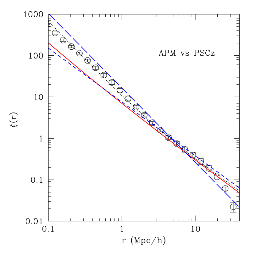
Figure 1: The APM correlation function measurements (circles with error bars) compared to four closed-form expressions for $\xi(r)$: two power-law toy models with slopes $\gamma=1.3$ (short-dashed line) and 1.8 (long-dashed line) and two more realistic, broken power-law empirical fits, given by eq. [3]. The latter two represent the PSCz (solid line) and the APM survey (dotted line). All four expressions for $\xi(r)$ assume $\sigma_{8}=0.83$.

where $r_{1}=2.33\,h^{-1}\,{\rm Mpc}$, $r_{2}=3.51\,h^{-1}\,{\rm Mpc}$, $\gamma_{1}=1.72$, $\gamma_{2}=1.28$, and $\sigma_{8}$ is a free parameter. If the PSCz galaxies follow the mass distribution, then $\sigma_{8}=\sigma_{8}^{\rm PSCz}=0.83$. The quantities $\sigma_{8}$ and $\xi(r)$ describe nonlinear matter density fluctuations at redshift zero. The PSCz fit with $\sigma_{8}=0.83$ in eq. (3) is plotted in figure 1, together with the APM correlation function measurements for comparison. For $\;r<15\,h^{-1}\,{\rm Mpc}$, the APM correlation function is well approximated by eq. [3] with $r_{1}=3.0\,h^{-1}\,{\rm Mpc}$, $r_{2}=2.5\,h^{-1}\,{\rm Mpc}$, $\gamma_{1}=1.9$ and $\gamma_{2}=1.1$. For $2\,h^{-1}\,{\rm Mpc}<r<15\,h^{-1}\,{\rm Mpc}$, which is the range of separations of interest here, the PSCz and APM correlation functions in figure 1 are almost indistinguishable. This provides an added reason to believe that choosing PSCz as a template for $\xi(r)$ was a good idea. To test the stability of our conclusions with respect to uncertainties regarding the small-$r$ behavior of $\xi(r)$, we will compare predictions for $v_{12}(r)$ based on PSCz parameters for eq. [3] with those based on the APM survey. To study the sensitivity of $v_{12}(r)$ and inferred cosmological parameters to the assumed slope of $\xi(r)$, we will also consider two simplified, pure power-law toy models, given by

$$\xi(r)\;=\;(\sigma_{8}/0.83)^{2}\;(r/r_{0})^{-\gamma}\;,$$ (4)

where $\gamma=1.3$ and 1.8, while $r_{0}=4.76\,h^{-1}\,{\rm Mpc}$ and $4.6\,h^{-1}\,{\rm Mpc}$, respectively.

3 Peculiar velocity surveys

We will now describe our measurements. Each redshift-distance survey provides galaxy positions, ${{\vec{r}}_{{\scriptscriptstyle A}}}$, and their radial peculiar velocities, $\,{s_{{\scriptscriptstyle A}}}={{\vec{r}}_{{\scriptscriptstyle A}}}\cdot{{\vec{v}}_{{\scriptscriptstyle A}}}/r_{\scriptscriptstyle A}\equiv{{\hat{r}}_{{\scriptscriptstyle A}}}\cdot{{\vec{v}}_{{\scriptscriptstyle A}}}\,$, rather than three-dimensional velocities ${{\vec{v}}_{{\scriptscriptstyle A}}}$. We use hats to denote unit vectors while indices $A,B=1,2,\ldots$ count galaxies in the catalogue. Consider a set of pairs $(A,B)$ at fixed separation $\,r=\bigl{|}{{\vec{r}}{{}_{{\scriptscriptstyle AB}}}}\bigr{|}\,$, where $\,{{\vec{r}}{{}_{{\scriptscriptstyle AB}}}}\equiv{{\vec{r}}_{{\scriptscriptstyle A}}}-{{\vec{r}}_{{\scriptscriptstyle B}}}\,$. To relate the mean radial velocity difference of a given pair to $v_{12}(r)$, we have to take into account a trigonometric weighting factor,

$$\langle\,{s_{{\scriptscriptstyle A}}}-{s_{{\scriptscriptstyle B}}}\,\rangle\;=\;v_{12}(r)\;{q_{{\scriptscriptstyle AB}}}\ \ \ \ \ \ \ {q_{{\scriptscriptstyle AB}}}\;\equiv\;{\hat{r}{{}_{{\scriptscriptstyle AB}}}}\cdot({{\hat{r}}_{{\scriptscriptstyle A}}}+{{\hat{r}}_{{\scriptscriptstyle B}}})/2\;=\;-{q_{{\scriptscriptstyle BA}}}\;.$$ (5)

To estimate $v_{12}$, we minimize the quantity $\chi^{2}(v_{12})\;=\;\sum_{{{}_{{\scriptscriptstyle A,B}}}}\,\left[({s_{{\scriptscriptstyle A}}}-{s_{{\scriptscriptstyle B}}})-{q_{{\scriptscriptstyle AB}}}\,v_{12}(r)\,\right]^{2}.$ The condition $\partial\chi^{2}/\,\partial v_{12}=0$ implies

$$v_{12}(r)\;=\;{{\sum_{{{}_{{\scriptscriptstyle A,B}}}}\,({s_{{\scriptscriptstyle A}}}-{s_{{\scriptscriptstyle B}}})\,{q_{{\scriptscriptstyle AB}}}}/\;{\sum_{{{}_{{\scriptscriptstyle A,B}}}}{q_{{\scriptscriptstyle AB}}}^{2}}}\;\;.$$ (6)

In this study we use following independent proper distance catalogues.

1. Mark III. This survey (Willick et al. 1995, 96, 97) contains five different types of data files: Basic Observational and Catalogue Data; Individual Galaxy Tully-Fisher (TF) and $D_{n}$-$\sigma$ Distances; Grouped Spiral Galaxy TF Distances; and Elliptical Galaxy Distances as in the Mark II (for TF and $D_{n}$-$\sigma$ methods, see Binney & Merrifield 1998). The subset we use here contains 2437 spiral galaxies with TF distance estimates. The total survey depth is over $120\,h^{-1}\,{\rm Mpc}$, with homogeneous sky coverage up to $30\,h^{-1}\,{\rm Mpc}$.

2. SFI (da Costa et al., 1996; Giovanelli et al., 1998; Haynes et al., 1999a,b). This is an all-sky survey, containing 1300 late type spiral galaxies with $I$-band TF distance estimates. The SFI catalogue, though sparser than Mark III in certain places, covers more uniformly the volume out to $70\,h^{-1}\,{\rm Mpc}$.

3. ENEAR (da Costa et al., 2000). This sample contains 1359 early type elliptical galaxies brighter than $m_{B}$ = 14.5 with $D_{n}$-$\sigma$ measured distances. ENEAR is a uniform, all-sky survey, probing a volume comparable to the SFI survey.

4. RFGC (Karachentsev et al., 2000). This catalogue provides a list of radial velocities, HI line widths, TF distances and peculiar velocities of 1327 spiral galaxies that was compiled from observations of flat galaxies from FGC (Karachentsev et al., 1993) performed with the 305 m telescope at Arecibo (Giovanelli et al., 1997). The observations are confined within the zone $0^{\circ}<\delta\leq+38^{\circ}$ accessible to the radio telescope.

Figure 2 shows our estimates of $v_{12}(r)$. Although the catalogues we used are independent, distinct and survey very different galaxy and morphology types, as well as different volumes and geometries, our results are robust and consistent with each other. The error bars are the estimated 1-$\sigma$ uncertainties in the measurement due to lognormal distance errors (around $15\%$), sparse sampling (shot noise), and finite volume of the sample (cosmic variance). For more details on error estimates used here, see Landy & Szalay (1992), Haynes et al. (1999a,b), and Ferreira et al. (1999).

The agreement among the $v_{12}(r)$ estimates from different surveys, plotted in figure 2 becomes even more impressive when compared to discrepancies between different estimates of a close cousin of our statistic, the pairwise velocity dispersion, $\sigma_{12}(r)$. The velocity dispersion appears to be less sensitive to the value of $\Omega_{m}$ than to the presence of rare, rich clusters in the catalogue and to galaxy morphology, with estimates of $\sigma_{12}$ at separations from one to a few Mpc varying from 300 to $800\,\rm km\,s^{-1}$ from one survey to another (Davis & Peebles, 1983; Żurek et al., 1994; Marzke et al., 1995; Zhao et al., 2002). The lack of systematic differences between $v_{12}(r)$ estimates in figure 2 is incompatible with the linear biasing theory unless the relative elliptical-to-spiral bias, $b_{\rm E}/b_{\rm S}$, is close to unity at separations $r>5\,h^{-1}\,{\rm Mpc}$, in agreement with our earlier studies (Juszkiewicz et al., 2000); for the same reason our results strongly disagree with recent semi-analytic simulations (Sheth et al., 2001; Yoshikawa et al., 2003).

In figure 3 we show the results for each of the catalogues we investigated, as in figure 2, but now we overlay the weighted mean of the individual catalogues. Since the results are robust, combining the catalogues reduces the errors and gives us a strong prediction for the parameter values. Figure 3 shows the results of our theoretical best fits: the solid (dotted) line follows the double power law correlation function using the PSCz (APM) correlation function (eq. [3]). Clearly, the slope differences in $\xi(r)$ at small separations do not affect $v_{12}(r)$ in the range of separations we consider. Moreover, given the error bars on $v_{12}$, the $\gamma=1.3$ power-law toy model prediction for $v_{12}(r)$, as well as the resulting best fit values of $\sigma_{8}$ and $\Omega_{m}$ are similar to those based on the APM and PSCz correlation functions. For $\sigma_{8}\approx 1$ and $\xi(r)\propto r^{-\gamma}$ at $r>10\,h^{-1}\,{\rm Mpc}$, linear theory applies and $v_{12}\propto r^{1-\gamma}$. Therefore all three of the models considered above give $v_{12}\propto r^{-0.3}$, in good agreement with the observed nearly flat $v_{12}(r)$ curve. All of the above does not apply to our $\gamma=1.8$ toy model, which is significantly steeper than the APM and PSCz $\xi(r)$ at large $r$, and for $\sigma_{8}\approx 1$, the $v_{12}(r)$ is expected to drop almost by half between 10 and $20\,h^{-1}\,{\rm Mpc}$. It is possible to flatten the $v_{12}(r)$ curve only by increasing $\sigma_{8}$ and extending the nonlinear regime to larger separations. The example considered here gives $\sigma_{8}=1.76$, in conflict with all other estimates of this parameter (see the discussion below). Correlation functions, steeper than APM or PSCz often appear in semi-analytic simulations and this example shows how $v_{12}(r)$ measurements can be used to constrain those models.

In figure 4 we plot the resulting 1,2,3 and $4\sigma$ likelihood contours in the $(\Omega_{m},\sigma_{8})$ plane. The quoted errors define the 1$\sigma$, or 68% statistical significance ranges in each of the two parameters and correspond to the innermost contour in figure 4. The low $\chi^{2}$ per degree of freedom is indicative of the correlations between $v_{12}(r)$ measurements at different separations $r$. One of the sources of correlations is the finite depth of our surveys. Note also that since we are dealing with pairs of galaxies, the same galaxy can in principle influence all separation bins. The contours derived using the PSCz correlation function (eq. [3]), are shown in the bottom right panel. The best fit values are

$$\Omega_{m}\,=\,0.30^{+0.17}_{-0.07}\;\;\;{\rm and}\;\;\;\sigma_{8}\,=\,1.13^{+0.22}_{-0.23}\;.$$ (7)

The likelihood contours based on the APM correlation function (with best fit values $\,\Omega_{m}=0.34^{+0.16}_{-0.14}\,$ and $\,\sigma_{8}=1.15^{+0.15}_{-0.20}$) and the $\gamma=1.3$ power-law model ($\,\Omega_{m}=0.23^{+0.15}_{-0.06}\,$ and $\,\sigma_{8}=1.20^{+0.20}_{-0.25}$) are similar. Our estimate of $\sigma_{8}$ agrees with the results of studies of clustering of galaxy triplets in real and Fourier space in three different surveys: the APM (Gaztañaga, 1995; Frieman & Gaztañaga, 1999), the PSCz (Feldman et al., 2001) and the 2dF (Verde et al., 2002). A similar value of $\sigma_{8}$ was recently inferred from the observed position of the inflection point in the APM $\xi(r)$ (Gaztañaga & Juszkiewicz, 2001). All of the above measurements are consistent with a $\sigma_{8}$ within 20% of unity. A $\sigma_{8}$ close to unity follows from maximum likelihood analysis of weak gravitational lensing (Van Waerbeke et al., 2002) after assuming $\Omega_{\Lambda}=0.7$, $\Omega_{m}=0.3$ and $h=0.7$. Measurements of the abundance of clusters (Bahcall et al., 2003) tend to give $\sigma_{8}$ closer to the lower end of our 68% interval if $\Omega_{m}=0.3$. The good agreement between these results, obtained with different methods, riddled with systematic errors of different nature, suggests that our estimates of statistical errors are reasonable and that the systematic errors are subdominant (unless there is an evil cosmic conspiracy of errors). The parameters in eq. [7] also agree with those inferred from the power spectrum of the anisotropy of the cosmic microwave background (CMB) temperature distribution on the sky: $\sigma_{8}=0.9\pm 0.1$, and $\Omega_{m}=0.29\pm 0.07$ (see Table 2 in Spergel et al. 2003). It is important to bear in mind, however, that unlike the CMB results, our estimates were obtained from the velocity and PSCz data alone, without the conventional priors. Therefore the $v_{12}(r)$ measurements combined with the CMB or the supernova data can be used to break the cosmological parameter degeneracy. Choosing $\gamma=1.8$, which is significantly steeper than the observed $\xi(r)$, gives $\Omega_{m}=0.14^{+0.06}_{-0.04}$ and $\sigma_{8}=1.76^{+0.34}_{-0.26}$ (figure 4, upper right), in conflict with all of the independent estimates of $\sigma_{8}$, discussed above. This suggests that the observed slope of the APM and PSCz correlation functions is close to the slope of the dark matter correlation function.

Acknowledgments: HAF wishes to acknowledge support from the NSF under grant number AST–0070702, the University of Kansas General Research Fund, the National Center for Supercomputing Applications, the Lady Davis Foundation and the Schonbrunn Fund at the Hebrew University, Jerusalem and by the Institute of Theoretical Physics at the Technion, Haifa, Israel. RJ wishes to thank Uriel Frisch for his hospitality at The Observatoire de la Côte d’Azur and also acknowledge support by a KBN grant 2P03D01719 (Poland), the Tomalla Foundation (Switzerland) and the Rose Morgan Visiting Professorship at the University of Kansas. PGF thanks the Royal Society. EG acknowledges support from INAOE, the Spanish MCyT, project AYA2002-00850 and EC-FEDER funding. This work began at the 1997 Summer Workshop at the Aspen Center for Physics, and we thank the Organizers.

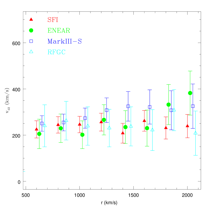
Figure 2: The pairwise velocities $v_{12}(r)$ for the four surveys. The Mark III-S $v_{12}(r)$ measurements come from our earlier work (Juszkiewicz et al., 2000). Clearly, the results from all surveys agree well with each other.

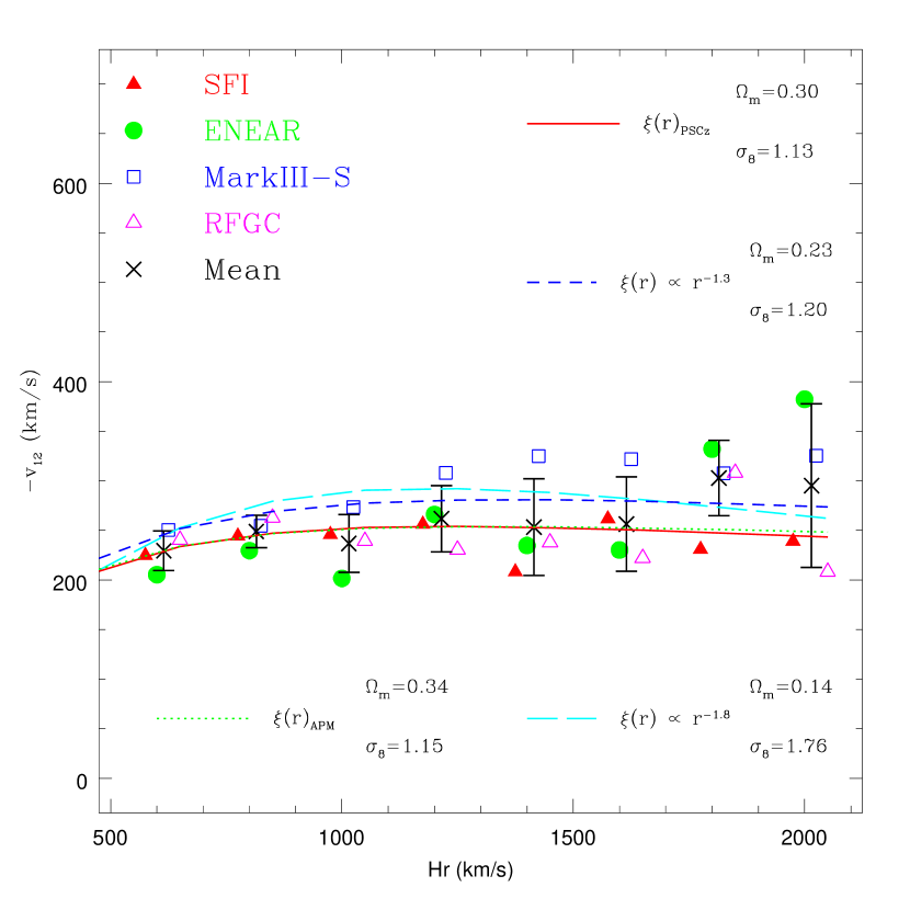
Figure 3: The crosses and the associated error bars show the weighted mean pairwise velocity, obtained by averaging over four surveys. Individual survey data points are also shown; we have suppressed their error bars for clarity. These direct measurements of $v_{12}$ are compared to four $v_{12}(r)$ curves, derived by assuming four different models of $\xi(r)$, plotted in figure 1. The labels identify best fit $\Omega_{m}$ and $\sigma_{8}$ parameters.

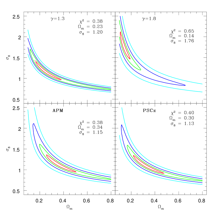
Figure 4: The results of the maximum likelihood analysis. The upper panels show results for power-law toy models, while the bottom panels are based on realistic representations of observations: the APM and PSCz data, respectively. Likelihood peak coordinates and the values of $\chi^{2}$ for each model are also indicated. The innermost contours define the 68%, or 1-$\sigma$ areas around the peaks. The remaining nested contours show the 2, 3 and 4-$\sigma$ boundaries.

References

- Bahcall et al. (2003) Bahcall, N. et al. , 2003, ApJ, 585, 182
- Binney & Merrifield (1998) Binney, J., & Merrifield, M., 1998, Galactic Astronomy (Princeton: Princeton University Press), p. 394
- Bridle et al. (2003) Bridle, S.L., et al. , 2003, astro-ph/0303180
- Courteau et al. (2000) Courteau, S.A., Strauss, M. A., & Willick, J. A., Eds., 2000, ASP Conf. Ser. 201, Cosmic Flows (San Francisco: ASP)
- da Costa et al. (1996) da Costa, L. N., et al. , 1996, ApJ, 468, L5
- da Costa et al. (2000) da Costa, L. N., et al. , 2000, AJ, 120, 95
- Davis & Peebles (1983) Davis, M. & Peebles, P. J. E., 1983, ApJ, 267, 465
- Feldman et al. (2001) Feldman, H. A., et al. , 2001, Phys. Rev. Lett., 86, 1434
- Ferreira et al. (1999) Ferreira, P. G., et al. , 1999, ApJ, 515, L1
- Frieman & Gaztañaga (1999) Frieman, J. A., & Gaztañaga, E., 1999, ApJ, 521, L83
- Gaztañaga (1995) Gaztañaga, E., 1995, ApJ, 454, 561
- Gaztañaga & Juszkiewicz (2001) Gaztañaga, E. & Juszkiewicz, R., 2001, ApJ, 558, L1
- Giovanelli et al. (1997) Giovanelli R., Avera A., Karachentsev I. D., 1997, AJ, 114, 122
- Giovanelli et al. (1998) Giovanelli, R., et al. , 1998, ApJ, 505, L91
- Hamilton & Tegmark (2002) Hamilton, A. J. S., & Tegmark, M. , 2002, MNRAS, 330, 506
- Haynes et al. (1999a,b) Haynes, M. P., et al. , 1999a, AJ, 117, 2039
- Haynes et al. (1999b) Haynes, M. P., et al. , 1999b, AJ, 117, 1668
- Juszkiewicz et al. (1999) Juszkiewicz, R., Springel, V. & Durrer, R., 1999, ApJ, 518, L25
- Juszkiewicz et al. (2000) Juszkiewicz, R., et al. , 2000, Sci, 287, 109
- Karachentsev et al. (1993) Karachentsev I. D., Karachentseva V. E., & Parnovsky S. L., 1993, Astron. Nachr., 314, 97
- Karachentsev et al. (2000) Karachentsev, I. D., et al. , 2000, Bull. Spec. Astrophys. Obs. N. Caucasus, 50, 5
- Landy & Szalay (1992) Landy S., & Szalay A., 1992, ApJ, 391, L494
- Marzke et al. (1995) Marzke, R. O., et al. , 1995, AJ, 110, 477
- Peebles (1980) Peebles, P. J. E., 1980, The Large-Scale Structure of the Universe, (Princeton: Princeton University Press), p. 170.
- Sheth et al. (2001) Sheth, R.K., et al. , 2001, MNRAS, 326, 463
- Spergel et al. (2003) Spergel, D.N., et al. , 2003, astro-ph/0302209
- Verde et al. (2002) Verde, L. et al. , 2002, MNRAS, 335, 432
- Van Waerbeke et al. (2002) Van Waerbeke, L. et al. , 2002, A&A, 393, 369
- Willick et al. (1995) Willick, J. A., et al. , 1995, ApJ, 446, 12
- Willick et al. (1996) Willick, J. A., et al. , 1996, ApJ, 457, 460
- Willick et al. (1997) Willick, J. A., et al. , 1997, ApJS, 109, 333
- Yoshikawa et al. (2003) Yoshikawa, K., Jing, J.P., & Börner, G., 2003, ApJ, 590, 654
- Zhao et al. (2002) Zhao, D., Jing, J. P. & Börner, G., 2002, ApJ, 581, 876
- Żurek et al. (1994) Żurek, W. H., et al. , 1994, ApJ, 431, 559