Gravitational lensing constraints on dark energy from modified Friedmann equations

Abstract

The existence of a dark energy component has usually been invoked as the most plausible way to explain the recent observational results. However, it is also well known that effects arising from new physics (e.g., extra dimensions) can mimic the gravitational effects of a dark energy through a modification of the Friedmann equation. In this paper we investigate some observational consequences of a flat, matter dominated and accelerating/decelerating scenario in which this modification is given by $H^{2}=g(\rho_{m},n,q)$ where $g(\rho_{m},n,q)$ is a new function of the energy density $\rho_{m}$, the so-called generalized Cardassian models. We mainly focus our attention on the constraints from statistical properties of gravitationally lensed quasars on the parameters $n$ and $q$ that fully characterize the models. We show that these models are in agreement with the current gravitationally lensed quasar data for a large interval of the $q-n$ parametric space. The dependence of the acceleration redshift (the redshift at which the universe begins to accelerate) on these parameters is also briefly discussed.

I Introduction

Over the last years, a considerable number of high quality observational data have transformed radically the field of cosmology. Results from distance measurements of type Ia supernovae (SNe Ia) perlmutter combined with Cosmic Microwave Background (CMB) observations bern and dynamical estimates of the quantity of matter in the universe calb seem to indicate that the simple picture provided by the standard cold dark matter scenario (SCDM) is not enough. These observations are usually explained by introducing a new hypothetical energy component with negative pressure, the so-called dark energy or quintessence peebles . If confirmed, the existence of this dark component would also provide a definitive piece of information connecting the inflationary flatness prediction with astronomical data.

On the other hand, it is also well known that not less exotic mechanisms like, e.g., geometrical effects from extra dimensions may be capable of explaning such observational results. The basic idea behind these “braneworld cosmologies” is that our 4-dimensional Universe would be a surface or a brane embedded into a higher dimensional bulk space-time to which gravity could spread rand . In some of these scenarios the observed acceleration of the Universe can be explained (without dark energy) from the fact that the bulk gravity sees its own curvature term on the brane acting as a negative-pressure dark component which accelerates the Universe dvali . A natural conclusion from these and other similar studies is that dark energy, or rather, the gravitational effects of a dark energy could actually be achieved from a modification of the Friedmann equation arising from new physics.

Following this reasoning, several authors have recently investigated cosmologies with a modified Friedmann equation from extra dimensions as an alternative explanation for the recent observational data. For example, Sahni & Shtanov sahni investigated a new class of braneworld models which admit a wider range of possibilities for dark energy than do the usual quintessence scenarios. For a subclass of the parameter values, they showed that the acceleration of the universe in this class of models can be a transient phenomena which could help reconcile an accelerating universe with the requirements of string/M-theory fis . Recently, Dvali & Turner turner explored the phenomenology and detectability of a correction on the Friedmann equation of the form $(1-\Omega_{m})H^{\alpha}/H_{o}^{\alpha-2}$, where $\Omega_{m}$ is the matter density parameter, $H$ is the Hubble parameter (the subscript “o” refers to present time) and $\alpha$ is a parameter to be adjusted by the observational data. Such a correction behaves like a dark energy with an effective equation of state given by $\omega=-1+\alpha/2$ in the recent past and like a cosmological constant ($\omega=-1$) in the distant future. Also based on extra dimensions physics, Freese & Lewis freese proposed the so-called Cardassian expansion, a model in which the universe is flat, matter dominated and currently accelerated. In the Cardassian universe, the new Friedmann equation is given by $H^{2}=g(\rho_{m})$, where $g(\rho_{m})$ is an arbitrary function of the matter energy density $\rho_{m}$. The first version of these scenarios had $g(\rho_{m})=A\rho_{m}+B\rho_{m}^{n}$, with the second term driving the acceleration of the universe at a late epoch after it becomes dominant (a detailed discussion for the origin of this Cardassian term from extra dimensions physics can be found in freese01 ). Although being completely different from the physical viewpoint, it was promptly realized that by identifying some free parameters Cardassian models and quintessence scenarios parameterized by an equation of state $p=\omega\rho$ predict the same observational effects in what concerns tests involving only the evolution of the Hubble parameter with the redshift freese . More recently, several forms for the function $g(\rho_{m})$ have been proposed freese1 . In particular, Wang et al. wang have studied some observational characteristics of a direct generalization of the original Cardassian model. According to these authors, the observational expressions in this new scenario are very different from generic quintessence cosmologies and fully determined by two dimensionless parameters, $n$ and $q$. Observational constraints from a variety of astronomical data have been also investigated recently, both in the original Cardassian model zong and in its generalized versions gat . Perhaps the most interesting feature of these models is that although being matter dominated, they may be accelerating and can still reconcile the indications for a flat universe ($\Omega_{\rm{total}}=1$) from CMB observations with the clustering estimates that point consistently to $\Omega_{m}\simeq 0.3$ with no need to invoke either a new dark component or a curvature term. In these scenarios, it happens through a redefinition of the value of the critical density freese ; wang (see also below).

The aim of this paper is to explore some observational consequences of these generalized Cardassian (GC) scenarios. We mainly focus our attention on the constraints that can be placed on the free parameters of the model ($n$ and $q$) from statistical properties of gravitationally lensed quasars. We show that for a large interval of these parameters, this class of models are fully compatible with the current gravitationally lensed quasar data. We also investigate the dependence of other observational quantities like the deceleration parameter, age-redshift relation and the acceleration redshift on the parameters $n$ and $q$.

This paper is organized in the following way. In Sec. II the field equations and distance formulas are presented. We also derive the expression for the deceleration parameter, age of the Universe and discuss the redshift at which the accelerated expansion begins. We then proceed to analyze the constraints from lensing statistics and on these scenarios in Sec. III. We end the paper by summarizing the main results in the conclusion Section.

II The model: basic equations

The modified Friedmann equation for GC models is wang

$$H^{2}=\frac{8\pi G\rho_{m}}{3}\left[1+\left(\frac{\rho_{card}}{\rho_{m}}\right)^{q(1-n)}\right]^{1/q},$$ (1)

where $n$ and $q$ are two free parameters to be adjusted by the observational data, $\rho_{{card}}=\rho_{o}(1+z_{{card}})^{3}$ is the energy density at which the two terms inside the bracket are equal and $\rho_{o}$ is the present day matter density. Note that for values of $n=0$ and $q=1$, GC scenarios reduce to Cold Dark Matter models with a cosmological constant ($\Lambda$CDM). As explained in wang , the first term inside the bracket dominates initially in such a way that the standard picture of the early universe is completely maintained. At a redshift $z_{{card}}$, these two terms become equal and, afterwards, the second term dominates, leading or not to an accelerated expansion (note, however, that $z_{card}$ is not necessarily the acceleration redshift. See, for instance, the discussion below on the deceleration parameter).

Evaluating Eq. (1) for present day quantities we find

$$H_{o}^{2}=\frac{8\pi G\rho_{o}}{3}\left[1+(1+z_{card})^{3q(1-n)}\right]^{1/q}.$$ (2)

From this equation, we see that $\rho_{o}$ is also the critical density that now can be written as

$$\rho_{o}=\rho_{c,old}\times\left[1+(1+z_{card})^{3q(1-n)}\right]^{-{1/q}},$$ (3)

where $\rho_{c,old}=1.88\times 10^{-29}h^{2}\rm{gm/cm^{3}}$ is the standard critical density and $h$ is the present day Hubble parameter in units of 100 ${\rm{km.s^{-1}Mpc^{-1}}}$. Note that for some combinations of the parameters $z_{card}$, $n$ and $q$ the critical density can be much lower than the one previously estimated. In other words it means that in the context of GC models it is possible to make the dynamical estimates of the quantity of matter that consistently point to $\rho_{o}\simeq(0.2-0.4)\rho_{c,old}$ compatible with the observational evidence for a flat universe from CMB observations and the inflationary flatness prediction with no need of a dark energy component (see freese for a more detailed discussion). In Fig. 1 we show a generalized version of the Figure 1 of freese in which the plane $z_{card}-n$ is displayed for selected values of $q$. The contours are labeled indicating the fraction of the standard critical density for different combinations of $z_{card}$ and $n$. In particular, the points inside the shadowed area delimited by the contours 0.2 - 0.4 are roughly consistent with the present clustering estimates calb .

From Eq. (3), we see that the observed matter density parameter in GC models can be written as

$$\Omega_{m}^{obs}=\frac{\rho_{o}}{\rho_{c,old}}=\left[1+(1+z_{card})^{3q(1-n)}\right]^{-{1/q}},$$ (4)

which, from now on, we will fix at 0.3 (in accordance to dynamical estimates of $\rho_{m}$ calb ) in order to discuss the acceleration redshift below and the lensing versus redshift test in the next section.

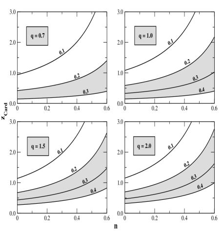
Figure 1: $z_{card}-n$ diagrams for the ratio $\rho_{o}/\rho_{c,old}$ (Eq. 4) and selected values of $q$. The contours are labeled indicating the corresponding fraction of the standard critical density. Points inside the shadowed area are roughly consistent with the present clustering estimates calb .

For the GC expansion parameterized by $n$ and $q$, the deceleration parameter as a function of the redshift has the following form

$$q(z)\equiv-\frac{\ddot{R}R}{\dot{R}^{2}}=-1+\frac{1}{2}\frac{d{\rm{ln}}f^{2}(z,\Omega_{m}^{obs},q,n)}{d{\rm{ln}}(1+z)},$$ (5)

where an overdot denotes derivative with respect to time, $R(t)$ is the cosmological scale factor and $f(z,\Omega_{m}^{obs},q,n)$ is given by Eq. (7). Figure 2 shows the behavior of the deceleration parameter as a function of redshift for selected values of $n$ and $q$. As discussed earlier, although completely dominated by matter, GC scenarios allow periods of accelerated expansion for some combinations of the parameters $n$ and $q$. Note that the present acceleration is basically determined by the value of $n$ and that the smaller its value the more accelerated is the present expansion for a given value of $q$. For example, for $q=1.5$ and $n=0$, GC models accelerate presently faster ($q_{o}\simeq-0.75$) than flat $\Lambda$CDM scenarios with $\Omega_{\Lambda}=0.7$ ($q_{o}\simeq-0.5$) although the acceleration redshift is almost identical ($z_{a}\simeq 0.7$) while for the same value of $q$ and $n=0.5$ we find $q_{o}\simeq-0.13$ and $z_{a}\simeq 0.52$. In order to make clear the difference between $z_{card}$ and $z_{a}$, for the latter values of $q$ and $n$, we find directly from Eq.(4) $z_{card}=1.06$. It means that although becoming dominant at $z_{card}\simeq 1$ the second term of Eq. (1) will drive an accelerated expansion only $\sim 1.7$ Gyr later, at $z_{a}\simeq 0.52$.

From the above equations, it is straightforward to show that the age-redshift relation is now given by (the total expanding age of the Universe $t_{o}$ is obtained by taking $z=0$)

$$t_{z}=\frac{1}{H_{o}}\int_{o}^{x^{\prime}}{dx\over xf(x,\Omega_{m}^{obs},q,n)},$$ (6)

where $x^{\prime}={R(t)\over R_{o}}=(1+z)^{-1}$ is a convenient integration variable and the dimensionless function $f(x,\Omega_{m}^{obs},q,n)$, obtained from Eqs. (1) and (4), is written as

$$f(x,\Omega_{m}^{obs},q,n)=\left\{\frac{\Omega_{m}^{obs}}{x^{3}}\left[1+\frac{(\Omega_{m}^{obs})^{-q}-1}{x^{-3q(1-n)}}\right]^{1/q}\right\}^{\frac{1}{2}}.$$ (7)

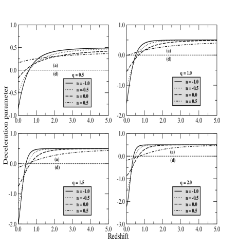
Figure 2: Deceleration parameter as a function of redshift for some selected values of $n$ and $q$ and $\Omega_{m}^{obs}=0.3$. The horizontal line labeled (a)/(d) ($q_{o}=0$) divides models with a accelerating (a) or decelerating (d) expansion at a given redshift. As discussed in the text, the present value of $q_{o}$ is basically determined by the value of $n$.

The comoving distance $r_{1}(z)$ to a light source located at $r=r_{1}$ and $t=t_{1}$ and observed at $r=0$ and $t=t_{o}$ can be expressed as

$$r_{1}(z)=\frac{1}{R_{o}H_{o}}\int_{x^{\prime}}^{1}{dx\over x^{2}f(x,\Omega_{m}^{obs},q,n)}.$$ (8)

In order to derive the constraints from lensing statistics in the next Section we shall deal with the concept of angular diameter distance. For the class of GC models here investigated, the angular diameter distance, $D_{LS}(z_{L},z_{S})={R_{o}r_{1}(z_{L},z_{S})/(1+z_{S})}$, between two objects, for example a lens at $z_{L}$ and a source (galaxy) at $z_{S}$, reads

$$D_{LS}(z_{L},z_{S}) = \frac{H_{o}^{-1}}{(1+z_{S})}\times$$

$$\times\int_{x^{\prime}_{S}}^{x^{\prime}_{L}}{dx\over x^{2}f(x,\Omega_{m}^{obs},q,n)}.$$

III Lensing constraints

In this Section we use statistics of gravitationally lensed quasars to place limits on the free parameters of GC scenarios. We work with a sample of 867 ($z>1$) high luminosity optical quasars which includes 5 lensed quasars. Our sample consists of data from the following optical lens surveys: HST Snapshot survey HST , Crampton survey Crampton , Yee survey Yee , Surdej survey Surdej , NOT Survey Jaunsen and FKS survey FKS . Since the main difference between the analysis performed in this Section and the previous ones that use gravitational lensing statistics to constrain cosmological parameters is the cosmological model that here is being considered, we refer the reader to previous works for detailed formulas and calculational methods (see, for instance, 1CSK ; lensing ). In order to perform our analysis we use the Schechter luminosity function with the lens parameters for E/SO galaxies taken from Madgwick et al. Mad , i.e., $\phi_{\ast}=0.27h^{3}\,10^{-2}{\rm{Mpc}}^{-3}$, $\alpha=-0.5$, $\gamma=4$, $v_{\ast}=220\,{\rm{km/s}}$ and $F^{*}=0.01$.

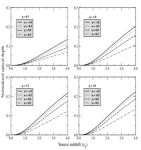
Figure 3: Normalized optical depth ($\tau/F^{*}$) as a function of the source redshift $z_{S}$ for some selected values of $n$ and $q$ and a fixed value of $\Omega_{m}^{obs}=0.3$.

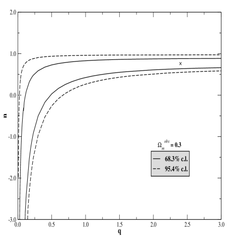
Figure 4: Confidence regions in the plane $n-q$ arising from lensing statistics for a fixed value of $\Omega_{m}^{obs}=0.3$. Solid (dashed) lines indicate contours of constant likelihood at $68.3\%$ c.l. ($95.4\%$ c.l.). The best-fit model is indicated by “$\times$”.

The total optical depth $\tau(z)$ along the line of sight from an observer at $z=0$ to a source at $z_{S}$ is given by

$$\tau(z_{S})=\frac{F^{*}}{30}\left[D_{OS}(1+z_{S})\right]^{3}R_{o}^{3}.$$ (10)

where $D_{OS}$ is the angular diameter distance (Eq. 9) from the observer to the source. In Fig. 3 for the fixed value of $\Omega_{m}^{obs}=0.3$ we show the normalized optical depth as a function of the source redshift for values of $q=$ 0.3, 1.0, 2.0 and 3.0 and $n=$ -1.0, -0.5, 0.0 and 0.5. Note that a decrease in the value of $n$ at fixed $\Omega_{m}^{obs}$ and $q$ tends to increase the optical depth for lensing. For $q=1.0$ at $z_{S}=3.0$, the value of $\tau/F^{*}$ for $n=0.5$ is down from that one for $n=-1.0$ by a factor of $\sim 2.02$, while the same values of $n$ and $q=2.0$ provides values for $\tau/F^{*}$ that are up from the previous ones only by a factor of $\sim$ 1.1 and 1.25, respectively. It clearly shows that the optical depth is a more sensitive function to the parameter $n$ than to the index $q$. As commented earlier, this particular feature is also noted for the other analyses discussed in this paper.

The likelihood function is defined by

$${\cal{L}}=\prod_{i=1}^{N_{U}}(1-p^{{}^{\prime}}_{i})\,\prod_{k=1}^{N_{L}}p_{k}^{{}^{\prime}}\,p_{ck}^{{}^{\prime}},$$ (11)

where $N_{L}$ is the number of multiple-imaged lensed quasars, $N_{U}$ is the number of unlensed quasars, and $p_{k}^{{}^{\prime}}$ and $p_{ck}^{{}^{\prime}}$ are, respectively, the probability of quasar $k$ to be lensed and the configuration probability (see 1CSK for details).

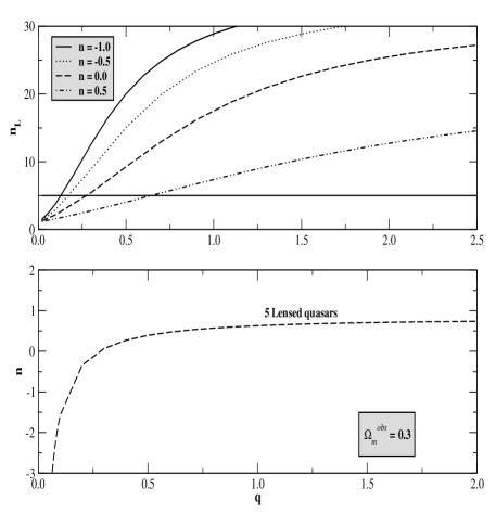
Figure 5: a) Predicted number of lensed quasars as a function of the parameter $q$ for selected values of $n$, $\Omega_{m}^{obs}=0.3$ and image separation $\Delta\theta\leq 4^{"}$. The horizontal solid line indicates $n_{L}=5$. b) Contour for five lensed quasars in the parametric space $q-n$.

Figure 4 shows contours of constant likelihood ($68.3\%$ and $95.4\%$) in the parameter space $n-q$. From the above equation we find that the maximum value of the likelihood function is located at $n=0.76$ and $q=2.4$ ($z_{card}\simeq 4.14$) which corresponds to a currently decelerated universe with $q_{o}\simeq 0.16$, i.e., apparently in contradiction to the SNe results (it is worth mentioning that a low-density decelerated model is not ruled out by SNe Ia data alone mesa , although such a model is strongly disfavored in the light of the recent CMB data). At the 1$\sigma$ level, however, almost the entire range of $q$ (if we consider for example $0<q\leq 4$) is compatible with the observational data for a fixed value of $\Omega_{m}^{obs}=0.3$. As observed earlier, this result suggests that a large class of GC scenarios is in accordance with the current gravitational lensing data. For the sake of comparison, we also note that the GC best-fit model obtained from our analysis and the one obtained for general quintessence scenarios with an equation of state $p_{x}=\omega_{x}\rho_{x}$ (XCDM) are very alike. For example, for XCDM models a similar analysis shows that the maximum value of the likelihood function is located at $\Omega_{\rm{m}}=0.0$ and $\omega_{x}=-0.2$ waga which corresponds to a decelerated model with a deceleration parameter $q_{o}=0.2$ and a total expanding age of $8.1h^{-1}$ Gyr. The best-fit for GC model also corresponds to a decelerated scenario with $q_{o}=0.16$ and a total age of the order of $8.7h^{-1}$ Gyr. We suspect that this similarity may be associated with the fact that the likelihood analysis is more sensitive to $n$ than to $q$ and, as commented earlier, the original Cardassian scenario (which depends only on $n$) and XCDM models predict very similar observational results freese . These particular values of $q$ and $n$ for the best-fit GC model provide a predicted age of the Universe old enough to accommodate some recent age estimates of high-$z$ objects. For example, at $z=1.55$ and $z=1.43$ Eq. (6) provides for $H_{o}=65$ ${\rm{kms^{-1}Mpc^{-1}}}$ $t_{z}=3.76$ Gyr and $t_{z}=4.01$ Gyr, respectively, i.e., values that are in agreement with the age estimates for the radio galaxies LBDS 53W091 and LBDS 53W069 dunlop . For the recent discovery of the quasar APM 08279+5255 komossa at $z=3.91$, however, these values of $q$ and $n$ provide $t_{z}=1.52$ Gyr while the age estimate for this object lies between 2.0 - 3.0 Gyr (a similar problem is also faced by the concordance $\Lambda$CDM model jailson ).

In Fig. 5a we show the expected number of lensed quasars, $n_{L}=\sum\,p_{i}^{{}^{\prime}}$ (the summation is over a given quasar sample), as a function of the index $q$ for some selected values of $n$. As indicated in the figure, the horizontal solid line stands for $n_{L}=5$, that is the number of lensed quasars in our sample. By this analysis, one finds that models with ($n$, $q$) = (-1.0, 0.13), (-0.5, 0.17), (0.0, 0.28) and (0.5, 0.65) predict exactly 5 lensed quasars. In Fig. 3b we display the contour for five lensed quasars in the parametric space $q-n$. As a general result, this analysis shows that a large number of models can accommodate the current gravitational lensing data.

IV Conclusion

The possibility of an accelerating universe from distance measurements of type Ia supernovae constitutes one of the most important results of modern cosmology. These observations naturally lead to the idea of a dominant dark energy component with negative pressure once all known types of matter with positive pressure generate attractive forces and decelerate the expansion of the universe. On the other hand, the realization that dark energy or the effects of dark energy could be a manifestation of a modification to the Friedmann equation arising from extra dimension physics has opened up an unprecedented opportunity to establish a more solid connection between particle physics and cosmology. Many “braneworld scenarios” have been proposed in the recent literature with most of them presenting interesting features which make them a natural alternative to the standard model. Here we have analyzed some observational consequences of one of these scenarios, the so-called generalized cardassian expansion recently proposed in Ref. wang . We have studied the observational constraints on the parameters $n$ and $q$ that fully characterize the model from statistical properties of gravitational lensing. From this analysis we have found that at $1\sigma$ level a large class of these scenarios is in agreement with the current lensing data with the maximum of the likelihood function located at $n=0.76$ and $q=2.4$ which corresponds to a decelerated model with $q_{o}=0.16$ and a predicted age of the Universe of the order of $t_{o}=8.7h^{-1}$ Gyr. Naturally, only with a more general analysis, possibly a joint investigation involving different classes of cosmological tests, it will be possible to show whether or not this class of models constitutes a viable alternative to the standard scenario.

- (1) S. Perlmutter et al., Nature, 391, 51 (1998); S. Perlmutter et al., Astrophys. J. 517, 565 (1999); A. Riess et al., Astron. J. 116, 1009 (1998)
- (2) P. de Bernardis et al., Nature 404, 955 (2000); A. E. Lange et al., Phys. Rev. D63, 042001 (2001); D. N. Spergel et al., astro-ph/0302209
- (3) R. G. Calberg et al., Astrophys. J. 462, 32 (1996); A. Dekel, D. Burstein and S. White S., In Critical Dialogues in Cosmology, edited by N. Turok World Scientific, Singapore (1997)
- (4) B. Ratra and P. J. E. Peebles, Phys. Rev. D37, 3406 (1988); M. S. Turner and M. White, Phys. Rev. D56, R4439 (1997); R. R. Caldwell, R. Dave and P. J. Steinhardt, Phys. Rev. Lett. 80, 1582 (1998); R. R. Caldwell, Braz. J. Phys. 30, 215 (2000); J. A. S. Lima and J. S. Alcaniz, Astrophys. J. 566, 15 (2002); P. J. E. Peebles and B. Ratra, astro-ph/0207347; J. C. Carvalho, J. A. S. Lima and I. Waga, Phys. Rev. D46 2404 (1992); M. C. Bento, O. Bertolami, A. A. Sen, Phys. Rev. D 66 (2002) 043507; A. Dev, D. Jain and J. S. Alcaniz, Phys. Rev. D 67, 023515 (2003); J. S. Alcaniz and J. M. F. Maia, Phys. Rev. D 67, 043502 (2003)
- (5) L. Randall, Science 296, 1422 (2002)
- (6) L. Randall and R. Sundrum, Phys. Rev. Lett. 83, 3370 (1999); G. Dvali, G. Gabadadze and M. Porrati, Phys. Lett. B485, 208 (2000); C. Deffayet, Phys. Lett. B 502, 199 (2001); R. Dick, Class. Quant. Grav. 18, R1 (2001); J. S. Alcaniz, Phys. Rev. D 65, 123514 (2002); M. D. Maia, E. M. Monte, J. M. F. Maia, astro-ph/0208223; A. Lue, hep-th/0208169
- (7) V. Sahni and Y. Shtanov, Int. J. Mod. Phys., 11, 1 (2002). astro-ph/0202346
- (8) W. Fischler, A. Kashani-Poor, R. McNees and S. Paban, JHEP 0107, 003 (2001)
- (9) G. Dvali and M. S. Turner, astro-ph/0301510
- (10) K. Freese and M. Lewis, Phys. Lett. B 540, 1 (2002)
- (11) D. J. Chung and K. Freese, Phys. Rev. D 61, 023511 (2000)
- (12) K. Freese, hep-ph/0208264
- (13) Y. Wang, K. Freese, P. Gondolo and M. Lewis, astro-ph/0302064
- (14) Z.-H. Zhu and M.-K. Fujimoto, Astrophys. J. , 581, 1 (2002); Astrophys. J. 585, 52 (2003); S. Sen and A. A. Sen, astro-ph/0211634; A. A. Sen and S. Sen, astro-ph/0303383
- (15) T. Multamaki, E. Gaztanaga and M. Manera, Submitted to MNRAS. astro-ph/0303526
- (16) D. Maoz et al., Astrophys. J. , 409, 28 (1993)
- (17) D. Crampton, R. McClure and J. M. Fletcher, Astrophys. J. 392, 23 (1992)
- (18) H. K. C. Yee, A. V. Filippenko and D. Tang, Astron. J. 105, 7 (1993)
- (19) J. Surdej et al., Astron. J. 105, 2064 (1993)
- (20) A. O. Jaunsen, M. Jablonski, B. R. Petterson and R. Stabell, Astron. Astrop., 300, 323 (1995)
- (21) C. S. Kochanek, E. E. Falco, and R. Schild, Astrophys. J. 452, 109 (1995)
- (22) C. S. Kochaneck, Astrophys. J. 466, 638 (1996)
- (23) L. F. Bloomfield Torres and I. Waga, MNRAS 279, 712 (1996); Z.-H. Zhu, Mod. Phys. Lett. A15, 1023 (2000); Z.-H. Zhu, Int. J. Mod. Phys. D9, 591 (2000); D. Jain, A. Dev and J. S. Alcaniz, Phys. Rev. D 66, 083511 (2002). astro-ph/0206224
- (24) D. S. Madgwick et al., astro-ph/0107197
- (25) A. Meszaros, Astrophys. J. 580, 12 (2002). astro-ph/0207558
- (26) I. Waga and A. P. M. R. Miceli, Phys. Rev. D 59, 103507 (1999)
- (27) J. Dunlop et al., Nature, 381, 581 (1996); J. Dunlop, in , ed. H. J. A. Rottgering, P. Best, & M. D. Lehnert, Dordrecht: Kluwer, 71 (1999); J. S. Alcaniz and J. A. S. Lima, Astrophys. J. , 521, L87
- (28) G. Hasinger, N. Schartel and S. Komossa, Astrophys. J. 573, L77 (2002); S. Komossa and G. Hasinger, in XEUS studying the evolution of the universe, G. Hasinger et al. (eds), MPE Report 281, 285 (astro-ph/0207321)
- (29) J. S. Alcaniz, J. A. S. Lima and J. V. Cunha, MNRAS 340, L39 (2003)