Abstract
The 2dF Galaxy Redshift Survey (2dFGRS) has produced a three-dimensional map of the distribution of 221,000 galaxies covering 5% of the sky and reaching out to a redshift . This is first map of the large-scale structure in the local Universe to probe a statistically representative volume, and provides direct evidence that the large-scale structure of the Universe grew through gravitational instability. Measurements of the correlation function and power spectrum of the galaxy distribution have provided precise measurements of the mean mass density of the Universe and the relative contributions of cold dark matter, baryons, and neutrinos. The survey has produced the first measurements of the galaxy bias parameter and its variation with galaxy luminosity and type. Joint analysis of the 2dFGRS and cosmic microwave background power spectra gives independent new estimates for the Hubble constant and the vacuum energy density, and constrains the equation of state of the vacuum.
Chapter 0 Cosmological Results from the
2dF Galaxy Redshift Survey
1 Introduction
The 2dF Galaxy Redshift Survey (2dFGRS) was made possible by the 2-degree Field (2dF) fiber spectrograph, which was specifically conceived as a tool for performing a massive redshift survey to precisely measure fundamental cosmological parameters. The state-of-the-art redshift surveys of the early 1990’s, such as the Las Campanas Redshift Survey (Shectman et al. 1996) and the IRAS Point Source Catalog redshift survey (Saunders et al. 2000), either did not cover sufficiently large volumes to be statistically representative of the large-scale structure, or covered large volumes too sparsely to provide precise measurements. An order-of-magnitude increase in the survey volume and sample size was needed to enter the regime of “precision cosmology,” and this became the foundational goal of the 2dFGRS.
The 2dF spectrograph can observe 400 objects simultaneously over a 2∘-diameter field of view (Taylor & Gray 1990; Lewis et al. 2002a), and was first placed on the Anglo-Australian Telescope (AAT) in November 1995. The first spectra were taken in mid-1996, and scheduled observations with 2dF at full functionality began in September 1997. The first major redshift survey observing run occurred in October 1997, with the survey passing 50,000 redshifts in mid-1999 (Colless 1999) and 100,000 redshifts in mid-2000. The first 100,000 redshifts and spectra were released publicly in June 2001 (Colless et al. 2001), and the 200,000-redshift mark was achieved toward the end of 2001. The survey observations were completed in April 2002, after 5 years and 272 nights on the AAT. The final survey is an order of magnitude larger than any previous redshift survey, and comparable to the ongoing redshift survey of the Sloan Digital Sky Survey (Bernardi, this volume).
The source catalog for the 2dFGRS was a revised and extended version of the APM galaxy catalog (Maddox et al. 1990), which was created by scanning the photographic plates of the UK Schmidt Telescope Southern Sky Survey. The survey targets were chosen to be galaxies with extinction-corrected magnitudes brighter than = 19.45 mag. The galaxies were distinguished from stars by the APM image classification algorithm described by Maddox et al., conservatively tuned to include all galaxies at the expense of also including a 5% contamination by stars.
The main survey regions were two declination strips, one in the southern Galactic hemisphere spanning 80∘15∘ around the South Galactic Pole (the SGP strip), and the other in the northern Galactic hemisphere spanning 75∘10∘ along the celestial equator (the NGP strip); in addition, there were 99 individual 2dF “random” fields spread over the southern Galactic cap (see Fig. 1). The large volume that is sparsely probed by the random fields allows the survey to measure structure on scales greater than would be permitted by the relatively narrow widths of the main survey strips. In total, the survey covers approximately 1800 deg2, and has a median redshift depth of = 0.11. An adaptive tiling algorithm was used to optimally place the 900 2dF fields over the survey regions, giving a highly complete and uniform sample of galaxies on the sky.

Redshifts were measured from 2dF spectra that covered the range from 3600 Å to 8000 Å at a resolution of 9.0 Å. Redshift measurements were obtained both from cross-correlation with template spectra and from fitting emission lines. All redshifts were visually checked and assigned a quality parameter in the range 1–5; accepted redshifts (3) were found to be 98% reliable and to have a typical uncertainty of 85 . The overall redshift completeness for accepted redshifts was 92%, although this varied with magnitude. The variation in the redshift completeness with position and magnitude is fully accounted for by the survey completeness mask (Colless et al. 2001; Norberg et al. 2002b).
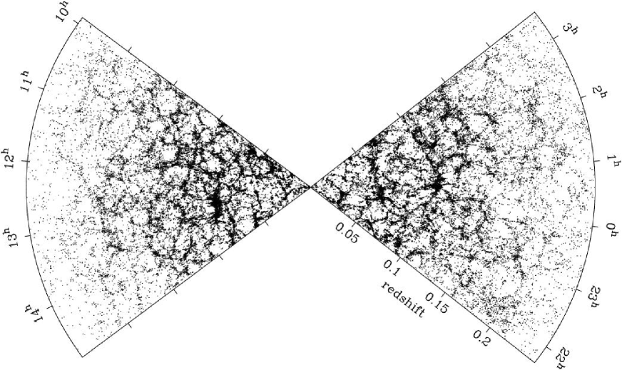
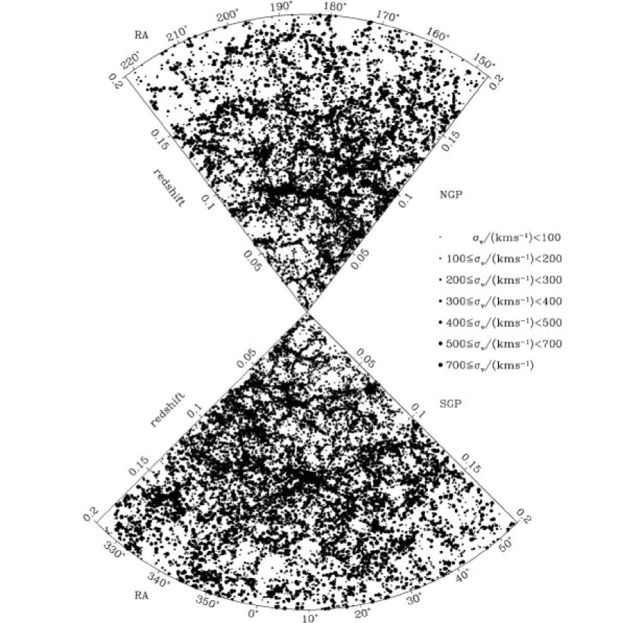
Figure 2 shows a thin slice through the three-dimensional map of over 221,000 galaxies produced by the 2dFGRS. This 3∘-thick slice passes through both the NGP strip (at left) and the SGP strip (at right). The decrease in the number of galaxies toward higher redshifts is an effect of the survey selection by magnitude — only intrinsically more luminous galaxies are brighter than the survey magnitude limit at higher redshifts. The clusters, filaments, sheets and voids making up the large-scale structures in the galaxy distribution are clearly resolved. The fact that there are many such structures visible in the figure is a qualitative demonstration that the survey volume comprises a representative sample of the Universe; the small amplitude of the density fluctuations on large scales is quantified by the power spectrum, as discussed in the next section.
2 The Large-scale Structure of the Galaxy Distribution
In cosmological models where the initial density fluctuations form a Gaussian random field, such as most inflationary models, the large-scale structure of the galaxy distribution in the linear regime is completely characterized in statistical terms by just two quantities: the mean density and the rms fluctuations in the density as a function of scale. The latter are quantified either through the two-point correlation function or the power spectrum, which are Fourier transforms of each other. However, a redshift survey does not determine the real-space positions of the galaxies, but rather the redshift-space positions, where the line-of-sight component is not the distance to the galaxy but the galaxy’s velocity. This velocity is the combination of the Hubble velocity (which is directly related to the distance) and the galaxy’s peculiar velocity (the motion produced by the gravitational attraction of the local mass distribution).
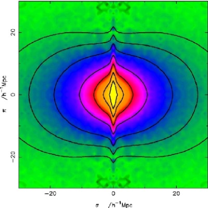
The statistical properties of the large-scale structure of the galaxy distribution observed in redshift space are summarized in Figure 3, which shows both the correlation function and the power spectrum obtained from the 2dFGRS. The structure on very large scales (several tens to hundreds of Mpc) is best represented by the power spectrum; on smaller scales, where peculiar velocities become more significant and the shape of the power spectrum (as well as the amplitude) differs between redshift space and real space, the redshift-space structure is most clearly shown in the two-dimensional correlation function (see §4 below).

The power spectrum, shown in the left panel of Figure 3, is well determined from the 2dFGRS on scales less than about 400 (wavenumbers ), and its shape is little affected by nonlinear evolution of the galaxy distribution on scales greater than about 40 (). Over this decade in scale, the power spectrum is well fitted by a cold dark matter (CDM) model having a shape parameter (Percival et al. 2001). For a Hubble constant around (i.e., ), this implies a mean mass density . The power spectrum also shows some evidence for acoustic oscillations produced by baryon-photon coupling in the early Universe (see §5).
The right panel of Figure 3 shows the redshift-space two-point correlations as a function of the separations along and across the line of sight, and reveals two main deviations from circular symmetry due to peculiar velocity effects. On intermediate scales, for transverse separations of a few tens of Mpc, the contours of the correlation function are flattened along the line of sight due to the coherent infall of galaxies as structures form in the linear regime. The detection of this effect in the 2dFGRS is a clear confirmation that large-scale structure grows by the gravitational amplification of density fluctuations (Peacock et al. 2001), and allows a direct measurement of the mean mass density of the Universe (see §5). The other effect is the stretching of the contours along the line of sight at small transverse separations. This is the finger-of-God effect due to the large peculiar velocities of collapsed structures in the nonlinear regime.
3 The Bias of the Galaxy Distribution
A fundamental issue in employing redshift surveys of galaxies as probes of cosmology is the relationship between the observed galaxy distribution and the underlying mass distribution, which is what cosmological models most directly predict. Some bias of the galaxies with respect to the mass is expected on theoretical grounds, but the nature and extent of the effect was not previously well determined. The large size of the 2dFGRS has allowed a thorough investigation of this question.
The simplest model for galaxy biasing postulates a linear relation between fluctuations in the galaxy distribution and fluctuations in the mass distribution: . In this case the galaxy power spectrum is related to the mass power spectrum by . Such a relationship is expected to hold in the linear regime (up to stochastic variations). The first-order relationship between galaxies and mass can therefore be determined by comparing the measured galaxy power spectrum to the matter power spectrum based on a model fit to the cosmic microwave background (CMB) power spectrum, linearly evolved to and extrapolated to the smaller scales covered by the 2dFGRS power spectrum. Applying this approach, Lahav et al. (2002) find that the linear bias parameter for an galaxy at zero redshift is , where is the optical depth due to reionization and is the spectral index of the primordial mass power spectrum.
An alternative way of determining the bias employs the higher-order correlations between galaxies in the intermediate, quasi-linear regime. The higher-order correlations are generated by nonlinear gravitational collapse, and so depend on the clustering of the dominant dark matter rather than the galaxies. Thus the stronger the higher-order clustering, the higher the dark matter normalization, and the lower the bias. An analysis of the bispectrum (the Fourier transform of the three-point correlation function) by Verde et al. (2002) yields , a result based solely on the 2dFGRS. Moreover, including a second-order quadratic bias term does not improve the fit of the bias model to the observed bispectrum.
For the blue-selected 2dFGRS sample, it therefore seems that galaxies are nearly unbiased tracers of the low-redshift mass distribution. However, this broad conclusion masks some very interesting variations of the bias parameter with galaxy luminosity and type (Fig. 4). Norberg et al. (2001, 2002a) show conclusively that the bias parameter varies with luminosity, ranging from for bright galaxies to for faint galaxies. The relation between bias and luminosity is well represented by the simple linear relation . They also find that, at all luminosities, early-type galaxies have a higher bias than late-type galaxies. A detailed comparison of the clustering of passive and actively star-forming galaxies by Madgwick et al. (2003) shows that at small separations, the passive galaxies cluster much more strongly, and the relative bias () is a decreasing function of scale. On the largest scales, however, the relative bias tends to a constant value of around 1.3.


4 Redshift-space Distortions
The redshift-space distortion of the clustering pattern can be modeled as the combination of coherent infall on intermediate scales and random motions on small scales. The compression of structures along the line of sight due to coherent infall is quantified by the distortion parameter (Kaiser 1987; Hamilton 1992). The random motions are adequately modeled by an exponential distribution, , where is the pairwise peculiar velocity dispersion (also called ).
The initial analysis of a subset of the 2dFGRS by Peacock et al. (2001) obtained best-fit values of and at an effective weighted survey luminosity and survey redshift . A more sophisticated reanalysis of the full 2dFGRS by Hawkins et al. (2003) obtains and , with and (right panel of Fig. 3). These results, using different fitting methods, are consistent, although the earlier result underestimates the uncertainties by 20%. Applying corrections based on the variation in the bias parameter with luminosity and a constant galaxy clustering model (Lahav et al. 2002) to the Hawkins et al. value for the distortion parameter yields .
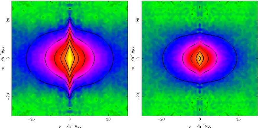
Madgwick et al. (2003) extend this analysis to a comparison of the active and passive galaxies, where the two-dimensional correlation function, , reveals differences in both the bias parameter on large scales and the pairwise velocity dispersion on small scales (Fig. 5). The distortion parameter is for passive galaxies and for active galaxies; over the range 8–20 the effective pairwise velocity dispersions are and for passive and active galaxies, respectively.
5 The Mass Density of the Universe
The 2dFGRS provides a variety of ways to measure the mean mass density of the Universe, along with the relative amounts of dark matter, baryons, and neutrinos.
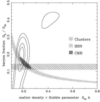
Fitting the shape of the galaxy power spectrum in the linear regime with a model including both CDM and baryons (Percival et al. 2001), and assuming that the Hubble constant is with a 10% uncertainty, yields a total mass density for the Universe of and a baryon fraction of (i.e., ). This analysis used 150,000 galaxies; a preliminary reanalysis of the complete final sample of 221,000 galaxies with the additional constraint that yields and (Peacock et al. 2003; left panel of Fig. 6). Including neutrinos as a further constituent of the mass allows an upper limit to be placed on their contribution to the total density, based on the allowable degree of suppression of small-scale structure due to the free streaming of neutrinos out of the initial density perturbations (right panel of Fig. 6). Elgarøy et al. (2002) obtain an upper limit on the neutrino mass fraction of 13% at the 95% confidence level (i.e., ). This translates to an upper limit on the total neutrino mass (summed over all species) of .

An alternative approach to deriving the total mass density is to use the measurements in the quasi-linear regime of the redshift-space distortion parameter , in combination with estimates of the bias parameter (Peacock et al. 2001; Hawkins et al. 2003). Using the Lahav et al. (2002) estimate for gives , while the Verde et al. (2002) value for gives .
6 Joint LSS-CMB Estimates of Cosmological Parameters
Stronger constraints on these and other fundamental cosmological parameters can be obtained by combining the power spectrum of the present-day galaxy distribution from the 2dFGRS with the power spectrum of the mass distribution at very early times derived from observations of the anisotropies in the CMB. A general analysis of the combined CMB and 2dFGRS data sets (Efstathiou et al. 2002) shows that, at the 95% confidence level, the Universe has a near-flat geometry (), with a low total matter density () and a large positive cosmological constant (, consistent with the independent estimates from observations of high-redshift supernovae).
![[Uncaptioned image]](/html/astro-ph/0305051/assets/x10.png)
Note: the best-fit parameters and rms errors are obtained by marginalizing over the likelihood distribution of the remaining parameters. Results are given for scalar-only and scalar+tensor models, and for the CMB power spectrum only and the CMB and 2dFGRS power spectra jointly.
If the models are limited to those with flat geometries (Percival et al. 2002), then tighter constraints emerge (see Table 1). In this case the best estimate of the matter density is , and the physical densities of CDM and baryons are and ; the latter agrees very well with the constraints from Big Bang nucleosynthesis. This analysis also provides an estimate of the Hubble constant () that is independent of, but in excellent accord with, the results from the Hubble Space Telescope Key Project. Comparing the uncertainties on the various parameters in the CMB-only and CMB+2dFGRS columns of Table 1 shows the very significant improvements that are obtained by combining the CMB and 2dFGRS data sets.
Joint fits to the 2dFGRS and CMB power spectra also constrain the equation of state parameter for the dark energy. Percival et al. (2002) find that in a flat Universe the joint power spectra, together with the Hubble Key Project estimate for , imply an upper limit of at the 95% confidence level.
7 The Galaxy Population
Alongside these cosmological studies, the 2dFGRS has also produced a wide range of results on the properties of the galaxy population, and provided strong new constraints for models of galaxy formation and evolution. Highlights in this area to date include: (1) precise determinations of the optical and near-IR galaxy luminosity functions (Cole et al. 2001; Norberg et al. 2002b); (2) a detailed characterization of the variations in the luminosity function with spectral type (Folkes et al. 1999; Madgwick et al. 2002); (3) a determination of the bivariate distribution of galaxies over luminosity and surface brightness (Cross et al. 2001); (4) a constraint on the space density of rich clusters of galaxies from the velocity dispersion distribution for identified clusters (De Propris et al. 2002); (5) separate radio luminosity functions for AGNs and star-forming galaxies (Sadler et al. 2002; Magliocchetti et al. 2002); (6) constraints on the star formation history of galaxies from the mean spectrum of galaxies in the local Universe (Baldry et al. 2002); (7) a measurement of the environmental dependence of star formation rates of galaxies in clusters (Lewis et al. 2002b); and (8) a comparison of the field and cluster luminosity functions for galaxies with difference spectral types (De Propris et al. 2003).
The next step will be to further investigate the correlations between these properties and the local environment of each galaxy, quantified through the local galaxy density or the new group and cluster catalog that has been constructed from the positions and velocity information in the 2dFGRS (Eke et al. 2003; see Fig. 7).
8 Conclusions
The measurement of cosmological parameters from the 2dFGRS has made a significant contribution to shaping the current consensus model for the fundamental properties of the Universe that has emerged from a range of independent observations, including the measurements of the CMB anisotropies, the distances to high-redshift supernovae, and Big Bang nucleosynthesis. The results obtained to date only represent a fraction of the information that can be extracted from the 2dFGRS on the properties of galaxies and their relation to the large-scale structure of the galaxy distribution. Much more is still to emerge from analysis of the survey, and from combining the 2dFGRS with other large surveys and with detailed follow-up observations.
Further information on the 2dF Galaxy Redshift Survey can be found on the WWW at http://www.mso.anu.edu.au/2dFGRS.
Acknowledgements. These results are presented on behalf of the 2dFGRS team: Ivan K. Baldry, Carlton M. Baugh, Joss Bland-Hawthorn, Sarah Bridle, Terry Bridges, Russell Cannon, Shaun Cole, Matthew Colless, Chris Collins, Warrick Couch, Nicholas Cross, Gavin Dalton, Roberto De Propris, Simon P. Driver, George Efstathiou, Richard S. Ellis, Carlos S. Frenk, Karl Glazebrook, Edward Hawkins, Carole Jackson, Bryn Jones, Ofer Lahav, Ian Lewis, Stuart Lumsden, Steve Maddox, Darren Madgwick, Peder Norberg, John A. Peacock, Will Percival, Bruce A. Peterson, Will Sutherland, and Keith Taylor. The 2dFGRS was made possible through the dedicated efforts of the staff of the Anglo-Australian Observatory, both in creating the 2dF instrument and in supporting it on the telescope.
References
- [1] Baldry, I., et al. 2002, ApJ, 569, 582
- [2] Cole, S., et al. 2001, MNRAS, 326, 255
- [3] Colless, M. M. 1999, Phil. Trans. R. Soc. Lond. A, 357, 105
- [4] Colless, M. M., et al. 2001, MNRAS, 328, 1039
- [5] Cross, N., et al. 2001, MNRAS, 324, 825
- [6] De Propris, R., et al. 2002, MNRAS, 329, 87
- [7] ——. 2003, MNRAS, submitted (astro-ph/0212562)
- [8] Efstathiou, G., et al. 2002, MNRAS, 330, L29
- [9] Eke, V., et al. 2003, in preparation
- [10] Elgarøy, Ø., et al. 2002, Phys. Rev. Lett., 89, 061301
- [11] Folkes, S., et al. 1999, MNRAS, 308, 459
- [12] Hamilton, A. J. S. 1992, ApJ, 385, L5
- [13] Hawkins, E., et al. 2003, MNRAS, submitted (astro-ph/0212375)
- [14] Kaiser, N. 1987, MNRAS, 227, 1
- [15] Lahav, O., et al. 2002, MNRAS, 333, 961
- [16] Lewis, I., et al. 2002a, MNRAS, 333, 279
- [17] ——. 2002b, MNRAS, 334, 673
- [18] Maddox, S. J., Efstathiou, G., Sutherland, W. J., & Loveday, J. 1990, MNRAS, 242, 43P
- [19] Madgwick, D. S., et al. 2002, MNRAS, 333, 133
- [20] ——. 2003, in preparation
- [21] Magliocchetti, M., et al. 2002, MNRAS, 333, 100
- [22] Norberg, P., et al. 2001, MNRAS, 328, 64
- [23] ——. 2002a, MNRAS, 332, 827
- [24] ——. 2002b, MNRAS, 336, 907
- [25] Peacock, J. A., et al. 2001, Nature, 410, 169
- [26] ——. 2003, in preparation
- [27] Percival, W. J., et al. 2001, MNRAS, 327, 1297
- [28] ——. 2002, MNRAS, 337, 1068
- [29] Sadler, E. M., et al. 2002, MNRAS, 329, 227
- [30] Saunders, W., et al. 2000, MNRAS, 317, 55
- [31] Shectman, S. A., Landy, S. D., Oemler, A., Tucker, D. L., Lin, H., Kirshner, R. P., & Schechter, P. L. 1996, ApJ, 470, 172
- [32] Taylor, K., & Gray P. 1990, Proc. SPIE, 1236, 290
- [33] Verde, L., et al. 2002, MNRAS, 335, 432