Double Inflation and the Low CMB Quadrupole

Abstract

Recent released WMAP data show a low value of quadrupole in the CMB temperature fluctuations, which confirms the early observations by COBE. In this paper we consider a model of two inflatons with different masses,$~{}V(\phi_{1},\phi_{2})={1\over 2}m_{1}^{2}\phi_{1}^{2}+{1\over 2}m_{2}^{2}\phi_{2}^{2}~{},$ $m_{1}>m_{2}$ and study its effects on CMB of suppressing the primordial power spectrum $P(k)$ at small $k$. Inflation is driven in this model firstly by the heavier inflaton $\phi_{1}$, then the lighter field $\phi_{2}$. But there is no interruption in between. We numerically calculate the scalar and tensor power spectra with mode by mode integrations, then fit the model to WMAP temperature correlations TT and the TE temperature-polarization spectra. Our results show that with $m_{1}\sim 10^{14}$ GeV and $m_{2}\sim 10^{13}$ GeV, this model solves the problems of flatness etc. and the CMB quadrupole predicted can be much lower than the standard power-law $\Lambda$CDM model.

Recently the Wilkinson Microwave Anisotropy Probe (WMAP) data Bennett ; Spergel ; Verde ; Peiris ; Komatsu have been released and it is shown that the data is consistent with the predictions of the standard ${\rm\Lambda}$CDM model with an almost scale-invariant, adiabatic and Gaussian primordial (scalar) fluctuations. However, there remain intriguing discrepancies between the model and the observations, which show the overprediction of the model on the amplitudes of fluctuations at both the largest and the smallest scales. In Ref.Spergel Spergel et al. include other data of the Cosmic Microwave Background(CMB)cbi ; acbar and Large Scale Structure(LSS)2df ; forest . They find that for power law $\Lambda$CDM model the best fit for the amplitude of fluctuations gradually drops as the probe of scale $k$ increases and the data supports for a nonzero running of the scalar spectrum index from blue to red at $2\sigma$ with $dn_{S}/d\ln k=-0.042^{+0.021}_{-0.020}$ Spergel . In Ref.seljak , the authors have questioned about the validity of the use of Lyman–$\alpha$ forest data forest , despite this a slightly running of the power spectrum index is still favored in the analysis of Refs. Spergel ; seljak ; Lewis ; Wang ; Caldwell . Especially, with a detailed reconstruction of the power spectrum Mukherjee and WangWang have shown a preferred feature at $k\sim 0.01$ Mpc^-1, consistent with a running of the index. And in Ref.Lewis Bridle et al. have stressed the importance of the data for the first three multipoles $l=2,3,4$ on the requirement for the running index.

Theoretically there have been studies in the literature since the release of the WMAP data on models of inflation which provide a running index required by the WMAP feng ; lidsey ; kawasaki ; huang ; CST . However, as shown in Ref.Spergel , the probability of finding a lower value of quadruple in the presence of a constant running of the spectral index is no more than 0.9 percent for a spatial flat $\Lambda$CDM cosmology. Indeed, the lack of CMB power on the large angular scales seen already in COBE cobe Fang and reinforced by WMAP is more challenging. This discrepancy may be due to cosmic variance. On the other hand, it probably gives a hint for new physics.

Recently several possibilities to $\bf{alleviate}$ the low-multipoles problem have been proposed in the literature Spergel ; Tegmark ; Efstathiou ; Bridle ; Lewis ; Linde ; Gaztanaga ; Cline which include considering the effect of a finite universeSpergel , the late time integrated Sachs-Wolf (ISW) effect by quintessenceBridle ; Linde , a non-flat universeEfstathiou , a suppression of the primordial fluctuationsLewis ; Linde ; Cline or different release of the dataTegmark ; Gaztanaga . In the framework of inflation, Contaldi et al inLinde have discussed two approaches to suppressing the large scale power. Beside the one of changing the inflaton potential, they have proposed another one of changing the initial conditions at the onset of inflation relative to the standard chaotic inflation modelchaotic . For the latter case, the inflaton has to be assumed in the kinetic dominated regime initially.

In this paper we consider a double inflation model and study the possibility of suppressing the lower multiples in the CMB. For a quantitative investigation we study a modeldouble :

$$V(\phi_{1},\phi_{2})={1\over 2}m_{1}^{2}\phi_{1}^{2}+{1\over 2}m_{2}^{2}\phi_{2}^{2}~{}.$$ (1)

The double inflation in the literature has been studied widely. And phenomenologically the model in (1) can be realized naturally in particle physics. For example, in the sneutrino inflation modelsYanagida ; Ellis , there are three sneutrinos which belong to three different families. Taking two of them degenerated, it is effectively a model of double inflation.

We assume in (1) that $\phi_{1}$ is heavier than $\phi_{2}$, i.e. $m_{1}>m_{2}$. The inflation is firstly driven by $\phi_{1}$, then by $\phi_{2}$, and there is no interruption in between. The transition takes place at $m_{\phi_{1}}\sim H$, where $H$ is the Hubble rate. When the transition happens $\phi_{1}$ starts to oscillate around the minimum of its potential. We denote the wavenumber of comoving mode which crosses the horizon around this moment as $k_{f}$. Choosing the model parameters so that $k_{f}$ corresponds to the scale around our current horizon, we will show in this paper that model (1) provides a scalar power spectrum much suppressed around $k_{f}$. With a set of the model parameters we will give a specific example of the initial power spectra and fit the spectra to WMAP data. Our results show that the spectrum with a feature is favored and lower CMB multipoles can be achieved by the spectrum with a feature provided by this model.

For the discussions on double inflation, we use the notations of Ref.Gordon . In a spatially flat Friedmann-Robertson-Walker (FRW) universe the evolution of the background fields for the potential given in (1) is described by the Klein-Gordon equation:

$$\ddot{\phi}_{I}+3H\dot{\phi}_{I}+V_{\phi_{I}}=0~{},$$ (2)

and the Friedmann equation:

$$H^{2}=(\frac{\dot{a}}{a})^{2}=\frac{8\pi G}{3}\left[\frac{1}{2}\dot{\phi}_{1}^{~{}2}+\frac{1}{2}\dot{\phi}_{2}^{~{}2}+V\right]\,,$$ (3)

where $I=1,2$, $a$ is the scale factor, the dot stands for time derivative and $V_{x}={\partial V}/{\partial x}$. Scalar linear perturbations to the FRW metric can be expressed generally as (we use the metric convention $+,-,-,-$):

$$ds^{2}=(1+2A)dt^{2}-2aB_{,i}dx^{i}dt-a^{2}[(1-2\psi)\delta_{ij}+2E_{,ij}]dx^{i}dx^{j}.$$ (4)

Thus the equation for the evolution of the perturbation $\delta\phi_{I}$ with comoving wavenumber $k$ is given by

$$\ddot{\delta\phi}_{I}+3H\dot{\delta\phi}_{I}+\frac{k^{2}}{a^{2}}\delta\phi_{I}+\sum_{J}V_{\phi_{I}\phi_{J}}\delta\phi_{J}=$$

$$-2V_{\phi_{I}}A+\dot{\phi}_{I}\left[\dot{A}+3\dot{\psi}+\frac{k^{2}}{a^{2}}(a^{2}\dot{E}-aB)\right]\,.$$ (5)

Defining the adiabatic field $\sigma$ and its perturbation as Gordon :

$$\dot{\sigma} = (\cos\theta)\dot{\phi}_{1}+(\sin\theta)\dot{\phi}_{2}\,,$$

$$\delta\sigma = (\cos\theta)\delta\phi_{1}+(\sin\theta)\delta\phi_{2}\,,$$ (6)

with

$$\cos\theta=-\frac{\dot{\phi_{1}}}{\sqrt{\dot{\phi_{1}}^{2}+\dot{\phi_{2}}^{2}}},\quad\sin\theta=-\frac{\dot{\phi_{2}}}{\sqrt{\dot{\phi_{1}}^{2}+\dot{\phi_{2}}^{2}}}\,.$$ (7)

The background equations (3) and (2) become

$$H^{2} = \frac{8\pi G}{3}(\frac{1}{2}\dot{\sigma}^{~{}2}+V)\,,$$

$$\ddot{\sigma} + 3H\dot{\sigma}+V_{\sigma}=0\,,$$ (8)

where $V_{\sigma}=(\cos\theta)V_{\phi_{1}}+(\sin\theta)V_{\phi_{2}}$. The comoving curvature perturbation is given by Gordon

$${\cal R}=\psi+\frac{H}{\dot{\sigma}}\delta\sigma\,.$$ (9)

We assume that there is no entropy perturbation, and this is consistent with the results of WMAP Peiris . Under this assumption, there is an adiabatic condition between $\delta\phi_{1}$ and $\delta\phi_{2}$:

$${\delta\phi_{1}\over\dot{\phi_{1}}}={\delta\phi_{2}\over\dot{\phi_{2}}}~{}.$$ (10)

So, the equation governing the evolution of adiabatic perturbation is the same as that in the single field inflation model mfb ; SL :

$$u^{\prime\prime}+(k^{2}-\frac{z^{\prime\prime}}{z})u=0~{},$$ (11)

where $u=-z{\cal R}$ and $z=a\dot{\sigma}/H$, the prime denotes the derivative with respect to conformal time $\eta$ ($\eta=\int\frac{dt}{a}$). The power spectrum of adiabatic perturbation is defined as

$$P_{\cal R}(k)=\frac{k^{3}}{2\pi^{2}}|\frac{u}{z}|^{2}~{},$$ (12)

which approaches a constant at late time as $k/aH\rightarrow 0$. Similarly for tensor perturbations the power spectrum is

$$P_{g}(k)=\frac{k^{3}}{2\pi^{2}}|\frac{v}{z}|^{2}~{},$$ (13)

where $v=a\Psi$, $\Psi$ is the linear tensor perturbation mfb ; SL and the equation of motion for $v$ is :

$$v^{\prime\prime}+(k^{2}-\frac{a^{\prime\prime}}{a})v=0~{}.$$ (14)

Using formulations above we are able to calculate the primordial power spectra with mode by mode integrationswenbin ; feng ; wangxl . Regarding the choices of the model parameters: initial values of $\phi_{1}$ and $\phi_{2}$, $m_{1}$ and $m_{2}$, we notice that $\phi_{1}$ is arbitrary with a weak prior to provide enough number of $e-folding$ to solve the flatness problemLinde ; Cline , $\phi_{2}$ mainly determines which $P_{R}$ correspond to the cosmological scale and the ratio of $m_{1}$ to $m_{2}$ determines the shape of $P_{R}$ with the absolute value of $m_{2}$ fixed by the WMAP normalization. For different values of $\phi_{2}$, the corresponding number of $e-folding$ to CMB scales will differ and the shape of $P_{R}$ will also get changed, as in the case of the single field inflation. The amplitude of $P_{R}(k)$ is to be determined by observations. In Fig.1 we show initial power spectra as a function of $\ln(k/k_{f})$. In the numerical calculationnote we have set $m_{1}=8m_{2}$ and $\phi_{2}=3.3M_{Pl}$ at the onset of inflation. This gives rise to $N(k_{f})=59.6$. We find such a value of $N(k_{f})$ is acceptable for fitting to WMAP data below. We also show in Fig.1 the behavior of the slow rolling(SR) parameters defined by $\epsilon\equiv-\dot{H}/H^{2}$ and $\delta\equiv\ddot{\sigma}/H\dot{\sigma}$  . One can see that these parameters change dramatically – this is why we use numerical calculations instead of the Stewart-Lyth analytical formulaSL ; wenbin ; Leach:2000yw .

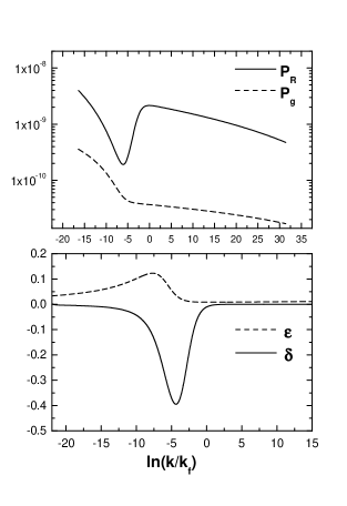
Figure 1: Initial power spectra and slow rolling parameters as a function of $\ln(k/k_{f})$. $N(k_{f})=59.6$

Now we fit the WMAP data with the primordial spectra in Fig.1. Our modified version of the publicly available CMBFAST cmbfast is based on Version 4.2 IEcmbfast and we have used the ”HP” choice to give exact CMB TT and TE power spectra. We also run with CAMBcamb ; IEcamb for a crosscheck on our results. We use a similar method to Ref.Linde , and set $\Omega_{\Lambda}$ and $\ln k_{f}$ as free parameters in our fit. Denoting $k_{c}=7.0\times 70./3/10^{5}\approx 1.6\times 10^{-3}$ Mpc^-1, we use 101 and 251 grid points with ranges $[0.68,0.77]$, and $[-19.6,5.4]$ respectively for $\Omega_{\Lambda}$ and $\ln(k_{f}/k_{c})$. At each point in the grid we use subroutines derived from those made available by the WMAP  team to evaluate the log likelihood with respect to the WMAP  TT and TE data Verde . Other parameters are fixed at $\Omega_{b}h^{2}=0.022$, $\Omega_{m}h^{2}=0.135$ and $\tau_{c}=0.17$ and $\Omega_{\rm tot}=1$ Spergel . The overall amplitude of the primordial perturbations has been used as a continuous parameter. Differing from Ref.Linde and Ref.Cline , we have included the tensor contributions in our fit to CMB. And for comparison, we also run the code without tensor.

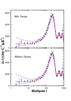
Figure 2: CMB anisotropies with primordial spectra shown in Fig.1 . The error bars are taken the same as Ref.Spergel . The upper and lower dashed lines show the 1-$\sigma$ confidence levels for lognormal distributions with cosmic variance limits. The middle solid lines show the models with the lowest quadrupoles.

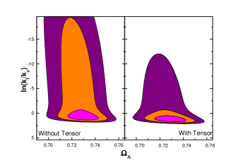
Figure 3: Two-dimesional contours in the $\ln(k_{f}/k_{c})$– $\Omega_{\Lambda}$ plane for our grids of model. $k_{c}\approx 1.6\times 10^{-3}$ Mpc^-1. The regions of different color show 68.3%, 95% and 99.7% confidence respectively.

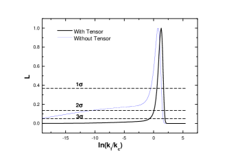
Figure 4: One-dimesional marginalized distributions for the values of $\ln(k_{f}/k_{c})$.

In Fig. 2 we show the resulting best–fit models obtained from the grids for the model considered. In the plots we take the same error bars on the binned WMAP results as Ref.Spergel . The regions between the two dashed lines are given by 1-$\sigma$ confidence levels for lognormal distributions as well as the cosmic variance limits. The cosmic variance factor is $1\pm\sqrt{2/(2l+1)}$. The middle solid lines show the models with the lowest quadrupoles. We get the minimum $\chi^{2}=1429.2$ when not including tensor and a slightly larger $\chi^{2}=1429.7$ with tensor for the best fit values. One can see the CMB low multipoles do have been suppressed in our model.

In Fig. 3 we plot the resulting $\chi^{2}$ values as functions of $\Omega_{\Lambda}$ and $\ln(k_{f}/k_{c})$. The contours shown are for $\Delta\chi^{2}$ values giving one, about two, and three $\sigma$ contours for two parameter Gaussian distributions. We find that the primordial spectrum with a feature is favored at more than 3-$\sigma$ level. However, when neglecting the tensor contribution, the significance reduces to only about 2-$\sigma$ level. In our model the ratio of tensor to scalar $r\equiv 8P_{g}/P_{R}$ reaches its minimum at $N\sim N(k_{f})$ and it gradually increases for smaller $N$ (larger $k$) and grows rapidly for larger $N$ (smaller $k$). And our $N(k_{f})$ corresponds to the region with the lowest value of $r$, which is consistent with WMAP group’s analysis that large tensor contribution is disfavored by current CMB observationsSpergel ; Peiris . The 1-$\sigma$ regions in Fig. 1 and Fig. 3 differ slightly when with and without tensor since $r$ is around its minimum in both cases.

We marginalize over $\Omega_{\Lambda}$ to obtain the one-dimensional probability distributions in $\ln(k_{f}/k_{c})$ shown in Fig. 4. For the spectra in Fig.1 when neglecting tensor contributions, we get $\ln(k_{f}/k_{c})=0.8$ with the maximum likelihood, corresponding to $k_{f}=3.6\times 10^{-3}$ Mpc^-1. We also have $k_{f}\sim 0$ at $2\sigma$ level. When taking into account tensor contributions, the maximum likelihood value of $\ln(k_{f}/k_{c})$ shift to 1.3 and we get $\ln(k_{f}/k_{c})=1.3^{+0.4}_{-0.7}$ at $1\sigma$, $1.3^{+0.6}_{-1.2}$ at $2\sigma$ and $1.3^{+0.7}_{-2.0}$ at $3\sigma$, corresponding to $k_{f}=6.0^{+3.0}_{-3.1}\times 10^{-3}$ Mpc^-1, $6.0^{+4.5}_{-4.3}\times 10^{-3}$Mpc^-1 and $6.0^{+5.7}_{-5.2}\times 10^{-3}$Mpc^-1 respectively. The difference in $\chi^{2}$ between the peak in the distributions and at $\ln(k_{f}/k_{c})=-19.6$ is found to be $\Delta\chi^{2}=6.1$ when not including tensor and $\Delta\chi^{2}=18.3$ when with tensor.

When considering tensor contributions in the two dimensional contour between $\ln(k_{f}/k_{c})$ and the normalized factor of the primordial scalar spectrum at $k=0.05$ Mpc^-1, we obtain $\ln(k_{f}/k_{c})=-0.8\sim 1.9$ and $P_{R}(0.05/Mpc)=2.48\sim 2.53\times 10^{-9}$ at $2\sigma$ level and we get $m_{1}=1.3\sim 1.4\times 10^{14}$ GeV. In contrast to the power law primordial spectrum with constant $n_{S}$ we run a similar code: we fix $\Omega_{b}h^{2}=0.022$, $\Omega_{m}h^{2}=0.135$ and $\tau_{c}=0.17$ and $\Omega_{\rm tot}=1$, varying $\Omega_{\Lambda}$ and $n_{S}$ with ranges [0.68,0.77], [0.91,1.07] and get a minimum $\chi^{2}=1432.7$. To characterize the pure power law primordial spectrum, one considers two parameters: $n_{S}$ and the amplitude. For our double inflation model four parameters are introduced to give the exact scalar and tensor spectra: $m_{1}$, $m_{1}/m_{2}$, $N(k_{f})$ (or equivalently $\phi_{2}$ at the onset of inflation) and $\ln(k_{f}/k_{c})$. This indicates our double inflation model is favored at $\sim 1.2\sigma$ compared with power law $\Lambda$CDM modelnote2 . In general, primordial power spectra with a feature or cutoff do generate a lower CMB TT quadrupole (which, however may not be sufficient)Lewis ; Linde ; Cline . A cutoff primordial spectrum also as pointed out in Ref.Cline makes the CMB TE multipoles lower. When combining these two effects, however, our calculations show that the primordial spectrum with a feature can work better than models with power law primordial spectra.

In conclusion, we have studied the possibility of suppressing the low multipoles in the CMB anisotropy with a model of double inflation. Our results show that with $m_{1}\sim 10^{14}$ GeV and $m_{2}\sim 10^{13}$ GeV which lies in the parameter space required by neutrino physics in the scenario of sneutrino inflationYanagida ; Ellis , this model fits to the WMAP data better than the standard power-law $\Lambda$CDM model.

We thank Dr. Mingzhe Li for discussions and Dr. H. H. Peiris for communications on WMAP data. We also thank the anonymous referee for comments and suggestions. This work was supported in part by National Natural Science Foundation of China and by Ministry of Science and Technology of China under Grant No. NKBRSF G19990754.

References

- (1) C. L. Bennett et al., astro-ph/0302207.
- (2) D. N. Spergel et al., astro-ph/0302209.
- (3) L. Verde et al., astro-ph/0302218.
- (4) H. V. Peiris et al., astro-ph/0302225.
- (5) E. Komatsuet al., astro-ph/0302223.
- (6) T. J. Pearson et al., astro-ph/0205388.
- (7) C. L. Kuo et al., astro-ph/0212289.
- (8) W. J. Percival et al., Mon. Not. Roy. Astr. Soc. 327, 1297 (2001).
- (9) R. A. C. Croft et al., Ap. J. 581, 20 (2002); N. Y. Gnedin and A. J. S. Hamilton, Mon. Not. Roy. Astr. Soc. 334, 107 (2002).
- (10) U. Seljak, P. McDonald, and A. Makarov, astro-ph/0302571.
- (11) S. L. Bridle, A. M. Lewis, J. Weller, and G. Efstathiou, astro-ph/0302306.
- (12) P. Mukherjee and Y. Wang, astro-ph/0303211.
- (13) For other approaches to suppressed small scale fluctuations see: R. R. Caldwell, M. Doran, C. M. Mueller, G. Schaefer and C. Wetterich, astro-ph/0302505.
- (14) B. Feng, M. Li, R.-J. Zhang, and X. Zhang, astro-ph/0302479.
- (15) J. E. Lidsey and R. Tavakol, astro-ph/0304113.
- (16) M. Kawasaki, M. Yamaguchi, and J. Yokoyama, hep-ph/0304161.
- (17) Q.-G. Huang and M. Li, hep-th/0304203.
- (18) D. J. Chung, G. Shiu and M. Trodden, astro-ph/0305193.
- (19) C. L. Bennett et al., Astrophys. J. 464, L1 (1996).
- (20) For papers relevant to suppressed CMB power on the largest angular scales on COBE see: Y.-P. Jing and L.-Z. Fang, Phys. Rev. Lett. 73,1882 (1994); J. Yokoyama, Phys. Rev. D59, 107303 (1999).
- (21) M. Tegmark, A. Oliveira-Costa, and A. J. S. Hamilton, astro-ph/0302496.
- (22) G. Efstathiou, astro-ph/0303127.
- (23) S. L. Bridle, O. Lahav, J. P. Ostriker, and P. J. Steinhardt, astro-ph/0303180.
- (24) C. R. Contaldi, M. Peloso, L. Kofman, and A. Linde, astro-ph/0303636.
- (25) J. M. Cline, P. Crotty and J. Lesgourgues, astro-ph/0304558.
- (26) E. Gaztanaga, J. Wagg, T. Multamaki, A. Montana and D. H. Hughes, astro-ph/0304178.
- (27) A. Linde, Phys.Lett.B 129, 177 (1983).
- (28) D. Polarski and A. A. Starobinsky, Nucl.Phys.B 385, 623 (1992); D. Polarski, Phys.Rev.D 49, 6319 (1994); D. Polarski and A. A. Starobinsky, Phys.Lett.B 356, 196 (1995); J. Lesgourgues and D. Polarski, Phys.Rev.D 56, 6425 (1997).
- (29) H. Murayama, H. Suzuki, T. Yanagida, and J. Yokoyama, Phys. Rev. Lett. 70, 1912 (1993); H. Murayama, H. Suzuki, T. Yanagida, and J. Yokoyama, Phys. Rev. D 50, 2356 (1994).
- (30) J. Ellis, M. Raidal, and T. Yanagida, hep-ph/0303242.
- (31) C. Gordon, D. Wands, B.A. Bassett, and R. Maartens, Phys. Rev. D63, 023506 (2001).
- (32) V. F. Mukhanov, H. A. Feldman and R. H. Brandenberger, Phys. Rept. 215, 203 (1992).
- (33) E. D. Stewart and D. H. Lyth, Phys. Lett. 302B, 171 (1993).
- (34) X. Wang et al., astro-ph/0209242.
- (35) D. H. Huang, W. B. Lin and X. M. Zhang Phys. Rev. D 62, 087302 (2000).
- (36) Since we have to resort to mode by mode integrations on and fit it to WMAP data, it is time consuming to make a full search in the model’s parameter space. We leave it for future investigations.
- (37) S. M. Leach and A. R. Liddle, Phys. Rev. D 63, 043508 (2001); S. M. Leach, M. Sasaki, D. Wands and A. R. Liddle,Phys. Rev. D 64, 023512 (2001).
- (38) U. Seljak and M. Zaldarriaga, Astrophys. J. 469, 437 (1996).
- (39) http://cmbfast.org/ .
- (40) A. Lewis, A. Challinor and A. Lasenby, Astrophys. J. 538, 473 (2000).
- (41) http://camb.info/ .
- (42) When global fits are applied to the comparison, e.g., all the background parameters vary, LSS and other CMB data are considered, the might get slightly changedCline .