The Cosmic Microwave Background and Helical Magnetic Fields:
the tensor mode

Abstract

We study the effect of a possible helicity component of a primordial magnetic field on the tensor part of the cosmic microwave background temperature anisotropies and polarization. We give analytical approximations for the tensor contributions induced by helicity, discussing their amplitude and spectral index in dependence of the power spectrum of the primordial magnetic field. We find that an helical magnetic field creates a parity odd component of gravity waves inducing parity odd polarization signals. However, only if the magnetic field is close to scale invariant and if its helical part is close to maximal, the effect is sufficiently large to be observable. We also discuss the implications of causality on the magnetic field spectrum.

I Introduction

The observed Universe is permeated with large scale coherent magnetic fields. It is still under debate whether these magnetic fields have been created by charge separation processes in the late Universe, or whether primordial seed fields are needed. Recently, it has been proposed vachaspati01 that also ‘helical’ magnetic fields, i.e. fields with a non-vanishing component in the direction of the current, ${\bf B\cdot(\nabla\times B)}\neq 0$, could be produced e.g. during the electroweak phase transition (see also brandenburg02 ).

Extended studies have already investigated effects of stochastic magnetic fields with vanishing helicity on the cosmic microwave background (CMB) (see jedamzik98 ; durrer00 ; grasso01 ; mack02 and others). In a seminal paper pogosian02 , Pogosian and collaborators have investigated the possibility that a helical magnetic field can induce correlations between the temperature anisotropy and the $B$ mode CMB polarization.

In this paper we want to go beyond that work. We determine all the effects on the CMB induced by a helical magnetic field. We shall actually show that, contrary to the statement in Ref. pogosian02 , a helical component also introduces pure CMB anisotropies and polarization. But of course its most remarkable effect is the above mentioned correlation of temperature anisotropy and $B$ polarization. We shall show that also a correlation between $E$ and $B$ polarization is induced.

In this paper we discuss only the tensor mode, gravitational waves, since the calculations for this case are simplest. Even if the resulting observational effects are small and may not be detectable, we find it interesting since it is completely new and contains several surprising elements. Furthermore, a fluid vorticity field or non parity invariant initial spectrum of gravitational waves produced during inflation could induce very similar effects; in that sense our results are more generic than their derivation.

In the next section, we discuss the magnetic field spectrum and define its symmetric and helical contributions. Then we compute the tensor component of the magnetic field energy momentum tensor which acts as a source for gravity waves. In Section IV we determine the induced gravity wave spectrum which also has a symmetric and a helical contribution. In Section V we compute the induced CMB temperature anisotropy and polarization spectra as well as the above mentioned correlations. Finally, we discuss our results and draw some conclusions. The paper is complemented by an appendix where details of calculations and tests of some approximations can be found.

II The magnetic field spectrum

We consider a primordial stochastic magnetic field created before equality, during the radiation-dominated epoch (or earlier). During this period of the evolution of the Universe, the conductivity of the primordial plasma on scales larger than the Silk scale $\lambda>\lambda_{S}$ is very high, effectively infinite ahonen96 . Hence, the ‘frozen-in’ condition holds, $\mathbf{E}=-\mathbf{v}\times\mathbf{B}$, where ${\mathbf{v}}$ is the plasma flux velocity, ${\mathbf{E}}$ is the electric field induced by plasma motions and ${\mathbf{B}}$ is the magnetic field. Moreover, large scale magnetic fields always induce anisotropic stresses, so that their energy density $B^{2}/8\pi$ must be a small perturbation, in order not to break the isotropy of the Friedmann Robertson Walker background. This allows us to apply linear perturbation theory. Both, the magnetic field energy and the plasma peculiar velocity are treated as first order perturbations; consequently, the energy density of the induced electric field will be $3$rd order in perturbations theory, and can be neglected. Also terms $E_{i}B_{j}$ are of second order and therefore neglected.

At sufficiently large scales, it is possible to neglect the effects of back reaction of the fluid on the evolution of the magnetic field: the time dependence decouples from the spatial structure, and, due to flux conservation, the magnetic field evolves like ${\mathbf{B}}(\eta,{\mathbf{x}})={\mathbf{B}}(\eta_{0},{\mathbf{x}})/a(\eta)^{2}$, where we use the normalization $a(\eta_{0})=1$ and a subscript $0$ denotes today. At smaller scales however, the interaction between the fluid and the magnetic field becomes important, leading mainly to two effects: on intermediated scale, the plasma undergoes Alfvén oscillations, and $B^{2}(k)\rightarrow B^{2}(k)\cos^{2}(v_{A}k\eta)$ (where $v_{A}^{2}=B^{2}/(4\pi(\rho+p))$ is the Alfvén velocity, here $B$ is the field averaged over a scale of order $v_{A}\eta$); on very small scales, the field is exponentially damped due to shear viscosity jedamzik98 ; subramanian98b ; subramanian98a ; durrer00 . As in Ref. durrer00 , we will account for this damping by introducing an ultraviolet cutoff at wavenumber $k_{D}(\eta)$ in the spectrum of $\mathbf{B}$ (see also mack02 ).

Following Refs. vachaspati01 ; pogosian02 , we introduce an helicity component $A(k)$ in the magnetic field two point correlation function:

$$\langle B_{j}({\mathbf{k}})B^{*}_{l}({\mathbf{k}^{\prime}})\rangle=\frac{(2\pi)^{3}}{2}\delta({\mathbf{k}}-{\mathbf{k}^{\prime}})[P_{jl}S(k)+i\epsilon_{jlm}\hat{k}_{m}A(k)]~{},$$ (1)

where $S(k)$ and $A(k)$ are respectively the symmetric and helical part of the magnetic field power spectrum. $P_{ij}\equiv\delta_{ij}-\hat{k}_{i}\hat{k}_{j}$ is the usual transverse plane projector satisfying the conditions $P_{ij}P_{jk}=P_{ik}$, $P_{ij}\hat{k}_{j}=0$, $\epsilon_{ijl}$ is the totally antisymmetric tensor, and $\hat{k}_{i}=k_{i}/k$. We use the Fourier transformation convention

$$B_{j}({\mathbf{k}})=\int d^{3}x\,\exp(i{\mathbf{k}}\cdot{\mathbf{x}})B_{j}({\mathbf{x}}),~{}~{}~{}~{}~{}~{}~{}~{}~{}~{}~{}~{}~{}~{}~{}~{}~{}~{}B_{j}({\mathbf{x}})={1\over{(2\pi)^{3}}}\int d^{3}k\,\exp(-i{\mathbf{k}}\cdot{\mathbf{x}})B_{j}({\mathbf{k}})~{}.$$ (2)

For simplicity, as in Refs. durrer00 ; mack02 and others, we shall assume that the magnetic field is a Gaussian random field. Then all the statistical information is contained in the two-point correlation function and the higher moments can be obtained via Wick’s theorem.

As explained in Ref. pogosian02 , the magnetic field helicity is determined by $\langle{\mathbf{B}}\cdot(\nabla\times{\mathbf{B}})\rangle$. For a better physical understanding of the effects which this new helicity term has on CMB anisotropies, it is useful to introduce the orthonormal ‘helicity basis’ $({\mathbf{e}}^{+},~{}{\mathbf{e}}^{-},~{}{\mathbf{e}}_{3}={\hat{\mathbf{k}}})$ (see also hu96 ; pogosian02 ), where

$${\mathbf{e}}^{\pm}({\bf k})=-\frac{i}{\sqrt{2}}({\mathbf{e}}_{1}\pm i{\mathbf{e}}_{2})~{},$$ (3)

and $({\mathbf{e}}_{1},~{}{\mathbf{e}}_{2},~{}{\mathbf{e}}_{3}={\hat{\mathbf{k}}})$ form a right-handed orthonormal basis with ${\mathbf{e}}_{2}={\hat{\mathbf{k}}}\times{\mathbf{e}}_{1}$. Under the transformation ${\mathbf{k}}\rightarrow-{{\mathbf{k}}}$ we choose $\mathbf{e}_{2}$ to change sign while $\mathbf{e}_{1}$ remains invariant. The basis $({\mathbf{e}}^{+},{\mathbf{e}}^{-},\hat{\mathbf{k}})$ has the following properties: ${\mathbf{e}}^{\pm}\cdot{\mathbf{e}}^{\mp}=-1$,  ${\mathbf{e}}^{\pm}\cdot{\mathbf{e}}^{\pm}=0$,  and ${\mathbf{e}}^{\pm}({{\mathbf{k}}})={\mathbf{e}}^{\mp}(-{{\mathbf{k}}})$, as well as $i\hat{{\mathbf{k}}}\times{\mathbf{e}}^{\pm}=\pm{\mathbf{e}}^{\pm}$.  The components of a vector with respect to this basis will be indicated by a superscript $\pm$. For a fixed ($k$-independent) basis we will instead use the usual Latin letters as indices. An arbitrary transverse vector ${\bf v}$ can be decomposed as ${\mathbf{v}}=v^{+}{\mathbf{e}}^{+}+v^{-}{\mathbf{e}}^{-}$. Here $v^{+}$ is the positive helicity component and $v^{-}$ is the negative helicity component.

With the definition (1), and the reality condition $(B^{\pm}({\bf k}))^{*}=-B^{\pm}(-{\mathbf{k}})$, we obtain the connection between the power spectra $S(k)$, $A(k)$ and the magnetic field components in the new basis:

$$-\langle B^{+}{(\mathbf{k})}B^{+}(-{\mathbf{k}^{\prime}})+B^{-}({\mathbf{k}})B^{-}(-{\mathbf{k}^{\prime}})\rangle = (2\pi)^{3}S(k)\delta({\mathbf{k}}-{\mathbf{k}^{\prime}})~{},$$ (4)

$$\langle B^{+}({\mathbf{k}})B^{+}(-{\mathbf{k}^{\prime})}-B^{-}({\mathbf{k}})B^{-}(-{\mathbf{k}^{\prime}})\rangle = (2\pi)^{3}A(k)\delta({\mathbf{k}}-{\mathbf{k}^{\prime}})~{}.$$ (5)

In other words, $A(k)$ represents the difference of the expectation values of the positive and negative helicity field components. If $A$ does not vanish, the left handed and right handed magnetic fields have different strength.

We assume that both the symmetric and helical terms of the magnetic field power spectrum (1) can be approximated by a simple power law pogosian02 :

$$S(k) = \left\{\begin{array}[]{ll}S_{0}~{}k^{n_{S}},&\mbox{ for }k<k_{D}\\ 0&\mbox{otherwise }\end{array}\right.$$

and

$$A(k) = \left\{\begin{array}[]{ll}A_{0}~{}k^{n_{A}},&\mbox{ for }k<k_{D}\\ 0&\mbox{otherwise}\end{array}\right.$$ (11)

where $S_{0}$, $A_{0}$ are the normalization constants, and $n_{S}$, $n_{A}$ the spectral indices of the symmetric and helical parts respectively.

With (II, 11), we can express the normalization constants $S_{0}$ and $A_{0}$ in terms of the averaged magnetic field energy density ${B_{\lambda}}^{2}\equiv\langle{\mathbf{B}}({\mathbf{x}})\cdot{\mathbf{B}}({\mathbf{x}})\rangle|_{\lambda}$, and the absolute value of the averaged helicity ${{\mathcal{B}}_{\lambda}}^{2}\equiv\lambda|\langle{\mathbf{B}}({\mathbf{x}})\cdot({\mathbf{\nabla}}\times{\mathbf{B}}({\mathbf{x}}))\rangle||_{\lambda}$ respectively, both smoothed over a sphere of comoving radius $\lambda$. ${\cal B}_{\lambda}$ measures the amplitude of helicity on the given comoving scale $\lambda$.

In order to calculate these quantities, we convolve the magnetic field and its helicity with a 3D-Gaussian filter function, so that $B_{i}\rightarrow B_{i}*f_{\lambda}$, where $\hat{f}_{\lambda}(k)=\exp(-\lambda^{2}k^{2}/2)$. The mean-square values $B^{2}_{\lambda}$ and ${\mathcal{B}}^{2}_{\lambda}$ are then given by the Fourier transform of the products of the corresponding spectra $S(k)$ and $kA(k)$ with the square of the filter function $\hat{f}_{\lambda}$:

$$B^{2}_{\lambda} = \frac{1}{(2\pi)^{3}}\int d^{3}k\,S(k)\hat{f}_{\lambda}(k)^{2}=\frac{S_{0}}{(2\pi)^{2}}\frac{1}{\lambda^{n_{S}+3}}\Gamma\left(\frac{n_{S}+3}{2}\right)~{},$$ (12)

$${\cal B}^{2}_{\lambda} = \frac{\lambda}{(2\pi)^{3}}\int d^{3}k\,k|A(k)|\hat{f}_{\lambda}(k)^{2}=\frac{|A_{0}|}{(2\pi)^{2}}\frac{1}{\lambda^{n_{A}+3}}\Gamma\left(\frac{n_{A}+4}{2}\right)~{}.$$ (13)

In order not to over-produce long range magnetic fields or helicity as $k\rightarrow 0$, we require for the spectral indices $n_{S}>-3$ and $n_{A}>-4$ (for $n_{A}\leq-3$ and $n_{A}\leq-4$ the integrals (12) and (13) diverge at small $k$).

Using (12), (13) and the definition of the magnetic field spectrum (1), we can rewrite expressions (4) and (5) in the form (see also pogosian02 )

$$-\langle B^{+}{(\mathbf{k})}B^{+}(-{\mathbf{k}^{\prime}})+B^{-}({\mathbf{k}})B^{-}(-{\mathbf{k}^{\prime}})\rangle = (2\pi)^{5}\frac{\lambda^{3}B^{2}_{\lambda}}{\Gamma\left(\frac{n_{S}+3}{2}\right)}(\lambda k)^{n_{S}}\delta({{\mathbf{k}}-{\mathbf{k}}^{\prime}})~{},$$ (14)

$$\langle B^{+}{(\mathbf{k})}B^{+}(-{\mathbf{k}^{\prime}})-B^{-}({\mathbf{k}})B^{-}(-{\mathbf{k}^{\prime}})\rangle = (2\pi)^{5}\frac{{\lambda^{3}\mathcal{B}}^{2}_{\lambda}}{\Gamma\left(\frac{n_{A}+4}{2}\right)}(\lambda k)^{n_{A}}\delta({{\mathbf{k}}-{\mathbf{k}}^{\prime}})~{},$$ (15)

for $k<k_{D}$ and $0$ for $k>k_{D}$.

Using that

$$\lim_{{\mathbf{k}}^{\prime}\rightarrow{\mathbf{k}}}|\langle(\hat{\mathbf{k}}\times{\mathbf{B}}({\mathbf{k}}))\cdot{\mathbf{B}}(-{\mathbf{k}}^{\prime})\rangle|\leq\lim_{{\mathbf{k}}^{\prime}\rightarrow{\mathbf{k}}}\langle{\mathbf{B}}({\mathbf{k}})\cdot{\mathbf{B}}(-{\mathbf{k}}^{\prime})\rangle$$

we can conclude that

$$S(k)\geq|A(k)|~{}.$$ (16)

Since $S(k)\propto\langle|{\mathbf{B}}|^{2}\rangle$, it is clear that $S(k)\geq 0$. The reality condition requires $A_{0}$ to be real, but it can be either positive or negative. For Eq. (16) to be valid on very small values of $k$ requires

$$n_{A}\geq n_{S}~{}.$$ (17)

Applying Eq. (16) also close to the upper cutoff $k_{D}$, we have in addition

$$|A_{0}|\leq S_{0}k_{D}^{n_{S}-n_{A}}~{}.$$ (18)

In terms of the magnetic fields on scale $\lambda$ this gives roughly

$${\cal B}_{\lambda}^{2}<B_{\lambda}^{2}(k_{D}\lambda)^{n_{S}-n_{A}}~{}.$$ (19)

Usually the damping scale is much smaller than the physical scale of interest, $\lambda$ so that $\lambda k_{D}\gg 1$. Therefore, if $n_{S}-n_{A}\neq 0$, the helical contribution is significantly suppressed on all scales $\lambda>\lambda_{D}=1/k_{D}$. As we now show, this is always the case if the magnetic field is causally produced.

Most mechanisms to produce magnetic fields with a helical component are causal. By this we mean that all correlations above a certain scale, usually some fraction of the Hubble scale at formation, have to vanish. If this is the case, causality implies an additional interesting constraint, which we now derive. For this we assume that the correlation functions $\langle B_{i}({\mathbf{x}})B_{j}({\mathbf{y}})\rangle$ and $\langle B_{i}({\mathbf{x}})(\nabla\times{\mathbf{B}}({\mathbf{y}}))_{j}\rangle$ have to vanish for $|{\mathbf{x}}-{\mathbf{y}}|>R$ for some scale $R$. Hence they are functions with compact support, which implies that their Fourier transforms, $P_{ij}S(k)$ and $\epsilon_{ijl}\hat{k}_{l}A(k)$ are analytic functions. Therefore, for sufficiently small values of $k$ they can be approximated by power laws as in Eqs. (II,11). Since $\hat{k}_{j}$ is not analytic but $k\hat{k}_{j}$ is, this implies

$$n_{S}\geq 2\quad\mbox{ and }~{}~{}~{}n_{A}\geq 1~{},$$ (20)

where $n_{S}$ has to be an even integer while $n_{A}$ has to be an odd integer. But since we need $n_{A}\geq n_{S}$, this leaves us with

$$n_{S} \geq 2\mbox{ , an even integer and }$$ (21)

$$n_{A} \geq 3\mbox{ , an odd integer}.$$ (22)

Causality together with the condition (16) leads to an additional suppression of helical fields on large scales. Also ordinary causal magnetic fields cannot be white noise but are severely suppressed on large scale due to the non-analytic pre-factor $P_{ij}$ in the power spectrum which is a simple consequence of the fact that magnetic fields are divergence free $\nabla\cdot{\mathbf{B}}=0$. This has already been discussed in Refs. durrer00 ; caprini02 . The causality constraint need not to be satisfied if the magnetic fields are generated before or during a period of inflation where the causal horizon diverges. For a detailed discussion of causality see Jcap .

III Magnetic Source term for tensor metric perturbations

The anisotropic stresses which act as source for metric perturbations are given by the magnetic field stress tensor jackson75

$$\tau_{ij}({\bf k})={1\over(2\pi)^{3}}{1\over 4\pi}\int d^{3}p\,[B_{i}({\bf p})B_{j}^{*}({\bf p-k})-{1\over 2}B_{l}({\bf p})B_{l}^{*}({\bf p-k})\delta_{ij}]~{}.$$ (23)

Here we are interested in the generation of gravitational waves, and consequently we need to extract the transverse and traceless part of $\tau_{ij}$. The form of a general projection to extract any mode (scalar, vector or tensor) from a generic tensorial perturbation can be found in dk98 . We make use of the tensor projector $T_{ijlm}=P_{il}P_{jm}-\frac{1}{2}P_{ij}P_{lm}$ (see also durrer00 ). The tensor contribution to $\tau_{lm}$ is given by

$$\Pi_{ij}=(P_{il}P_{jm}-\frac{1}{2}P_{ij}P_{lm})\tau_{lm}~{}.$$ (24)

Moreover, since the magnetic field is a stochastic variable, we need to calculate the two point correlation tensor of $\tau_{ij}({\mathbf{k}})$, which takes the form

$$\langle\tau_{ij}({\mathbf{k}})\tau^{*}_{lm}({\mathbf{k}^{\prime}})\rangle={1\over(4\pi)^{2}}{1\over(2\pi)^{6}}\int d^{3}p\int d^{3}q\,\langle B_{i}({\mathbf{p}})B_{j}({{\mathbf{k}}-{\mathbf{p}}})B_{l}({-{\mathbf{q}}})B_{m}({{\mathbf{q}}-{\mathbf{k}}^{\prime}})\rangle+\cdots\delta_{ij}+\cdots\delta_{lm}~{},$$ (25)

and we are not interested in terms proportional to $\delta_{ij}$ and $\delta_{lm}$ , which after being projected out will not contribute to the final result for the tensor perturbation $\langle\Pi_{ij}\Pi_{lm}\rangle$ (see appendix A. in mack02 ). Before applying the tensor projection, we can simplify the right hand side of (25) using Wick’s theorem, expressing the four point correlators in terms of the two point ones,

$$\langle B_{i}({\mathbf{k}}_{i})B_{j}({\mathbf{k}}_{j})B_{l}({\mathbf{k}}_{l})B_{m}({\mathbf{k}}_{m})\rangle = \langle B_{i}({\mathbf{k}}_{i})B_{j}({\mathbf{k}}_{j})\rangle\langle B_{l}({\mathbf{k}}_{l})B_{m}({\mathbf{k}}_{m})\rangle$$ (26)

$$+ \langle B_{i}({\mathbf{k}}_{i})B_{l}({\mathbf{k}}_{l})\rangle\langle B_{j}({\mathbf{k}}_{j})B_{m}({\mathbf{k}}_{m})\rangle$$

$$+ \langle B_{i}({\mathbf{k}}_{i})B_{m}({\mathbf{k}}_{m})\rangle\langle B_{j}({\mathbf{k}}_{j})B_{l}({\mathbf{k}}_{l})\rangle~{}.$$

Since the two point correlation function given in Eq. (1) is not symmetric, we are not allowed to change the order of indices $i,j,l,m$ inside an expectation value. With Eq. (1) we can then compute the correlation function (25) which consists of a purely symmetric part proportional to $\int d^{3}pS(p)S(|{\mathbf{k}}-{\mathbf{p}}|)$ , a purely helical part proportional to $\int d^{3}pA(p)A(|{{\mathbf{k}}-{\mathbf{p}}|})$ , and mixed term, $i\int d^{3}pS(p)A(|{\mathbf{k}-{\mathbf{p}}|})$ (the full expressions are given in Appendix A, Eq. (113)). The first two terms contribute to the symmetric part of the two point correlation function of the tensor source, while the two latter terms give rise to a helical contribution. To express them we now introduce the two point correlation function for the tensor source, which can be parameterized as

$$\langle\Pi_{ij}({\mathbf{k}})\Pi^{*}_{lm}({\mathbf{k}^{\prime}})\rangle\equiv\frac{(2\pi)^{3}}{4}\left[{\mathcal{M}}_{ijlm}f(k)+i{\cal A}_{ijlm}g(k)\right]\delta({\mathbf{k}-{\mathbf{k}}^{\prime}})~{},$$ (27)

where the tensors ${\mathcal{M}}_{ijlm}$ and ${\mathcal{A}}_{ijlm}$ are given by

$${\mathcal{M}}_{ijlm} \equiv P_{il}P_{jm}+P_{im}P_{jl}-P_{ij}P_{lm}~{},$$ (28)

$${\cal A}_{ijlm} \equiv {{\hat{\mathbf{k}}}_{q}\over 2}(P_{jm}\epsilon_{ilq}+P_{il}\epsilon_{jmq}+P_{im}\epsilon_{jlq}+P_{jl}\epsilon_{imq})~{}.$$ (29)

Clearly, both ${\cal M}_{ijlm}$ and ${\cal A}_{ijlm}$ are symmetric in the first and second pair of indices. ${\cal M}_{ijlm}$ is also symmetric under the exchange of $ij$ with $lm$ while ${\cal A}_{ijlm}$ is anti-symmetric under this permutation. We shall often use simple properties like

$${\cal M}_{ijij} = 4~{},\quad{\cal M}_{iilm}={\cal M}_{ijll}=0$$ (30)

$$P_{qi}{\mathcal{M}}_{ijlm} = {\mathcal{M}}_{qjlm}~{},\quad P_{qi}{\mathcal{A}}_{ijlm}={\mathcal{A}}_{qjlm}$$ (31)

$${\mathcal{M}}_{ijlm}{\mathcal{M}}_{ijlm} = {\mathcal{A}}_{ijlm}{\mathcal{A}}_{ijlm}=8$$ (32)

$${\cal A}_{ijlm}{\cal M}_{ijlm} = 0~{},\quad{\cal A}_{ijij}={\cal A}_{iijl}={\cal A}_{ijll}=0~{}.$$ (33)

According to Eq. (24), we have now to act on $\langle\tau_{ab}({\mathbf{k}})\tau^{*}_{cd}({\mathbf{k}^{\prime}})\rangle$ with the tensor projector

$${\cal P}^{abcd}_{ijlm}(\hat{\mathbf{k}},\hat{\mathbf{k}}^{\prime})=(P_{ia}P_{jb}-{1\over 2}P_{ij}P_{ab})({\hat{\mathbf{k}}})(P_{lc}P_{md}-{1\over 2}P_{lm}P_{cd})({\hat{\mathbf{k}}^{\prime}})~{}.$$ (34)

In these calculations we don’t need to care about the position (up or down) of Latin indices as they are always contracted by a Kronecker $\delta$. The symmetric and antisymmetric parts of Eq. (27) are invariant under the application of the projector (34), so that it is easy to separate the symmetric and helical parts of the source spectrum, $f(k)$ and $g(k)$:

$$(2\pi)^{3}\delta({\mathbf{k}}-{\mathbf{k}}^{\prime})f(k) = {1\over 2}{\mathcal{M}}_{abcd}\langle\tau_{ab}({\mathbf{k}})\tau^{*}_{cd}({\mathbf{k}^{\prime}})\rangle$$ (35)

$$(2\pi)^{3}\delta({\mathbf{k}}-{\mathbf{k}}^{\prime})g(k) = {-i\over 2}{\cal A}_{abcd}\langle\tau_{ab}({\mathbf{k}})\tau^{*}_{cd}({\mathbf{k}^{\prime}})\rangle~{}.$$ (36)

Moreover, by applying the tensor ${\mathcal{M}}_{ijlm}$ to Eq. (113) of Appendix A, we obtain (the first term of this has already been computed in Refs. durrer00 ; caprini02 ; mack02 )

$$f(k)=\frac{2}{(4\pi)^{5}}\int d^{3}p\,\left[\right.S(p)S(|{\mathbf{k}-{\mathbf{p}}}|)(1+\gamma^{2})(1+\beta^{2})+4A(p)A(|{\mathbf{k}-{\mathbf{p}}}|)(\gamma\beta)\left.\right]~{},$$ (37)

where $\gamma={\hat{\mathbf{k}}}\cdot{\hat{\mathbf{p}}}$ and $\beta={\hat{\mathbf{k}}}\cdot(\widehat{{\bf k-p}})$. Note that the square of the helical part of the magnetic field spectrum (1) contributes to the symmetric part of the source spectrum. This is not surprising, since the product of two quantities with odd parity has even parity. The antisymmetric part of the source spectrum is obtained by acting with ${\mathcal{A}}_{ijlm}$ on Eq. (113) of Appendix A. It is given by the mixed terms,

$$g(k)=\frac{8}{(4\pi)^{5}}\int d^{3}p\,S(p)A(|{\mathbf{k}-{\mathbf{p}}}|)(1+\gamma^{2})\beta~{}.$$ (38)

We can also express the correlator (27) in terms of the basis $e^{\pm}_{ij}$ introduced in hu96 ,

$${e}^{\pm}_{ij}=-\sqrt{\frac{3}{8}}({\bf e}_{1}\pm i{\bf e}_{2})_{i}\times({\bf e}_{1}\pm i{\bf e}_{2})_{j}~{}.$$ (39)

These form a basis of tensor perturbations, satisfying the transverse-traceless condition $\delta_{ij}{e}^{\pm}_{ij}=0$, ${\hat{k}}_{i}{e}^{\pm}_{ij}=0$ and ${e}^{\pm}_{ij}{e}^{\mp}_{ij}=3/2$. Positive circularly polarized gravity waves are proportional to $e^{+}_{ij}$, while negative circularly polarized gravity waves are given by the coefficient of $e^{-}_{ij}$. In this basis $\Pi_{ij}$ is expressed as

$$\Pi_{ij}({\bf k})\equiv e^{+}_{ij}\Pi^{+}({\mathbf{k}})+e^{-}_{ij}\Pi^{-}({\mathbf{k}})~{}.$$ (40)

We can rewrite $f(k)$ and $g(k)$ in terms of the components $\Pi^{\pm}$ as

$$(2\pi)^{3}\delta({\mathbf{k}}-{\mathbf{k}}^{\prime})~{}f(k)\equiv(2\pi)^{3}\delta({\mathbf{k}}-{\mathbf{k}}^{\prime})~{}|\Pi(k)|^{2} = \frac{3}{2}~{}\langle\Pi^{+}{(\mathbf{k})}\Pi^{+*}({\mathbf{k}^{\prime}})+\Pi^{-}({\mathbf{k}})\Pi^{-*}({\mathbf{k}^{\prime}})\rangle~{},$$ (41)

$$(2\pi)^{3}\delta({\mathbf{k}}-{\mathbf{k}}^{\prime})~{}g(k) = -\frac{3}{2}~{}\langle\Pi^{+}{(\mathbf{k}})\Pi^{+*}({\mathbf{k}^{\prime}})-\Pi^{-}({\mathbf{k}})\Pi^{-*}({\mathbf{k}^{\prime}})\rangle~{}.$$ (42)

Here we have used the form of $\cal M$ and $\cal A$ in this basis,

$${\cal M}_{ijlm} = {4\over 3}\left[e^{+}_{ij}\otimes e^{-}_{lm}+e^{-}_{ij}\otimes e^{+}_{lm}\right]$$

$${\cal A}_{ijlm} = {4i\over 3}\left[e^{+}_{ij}\otimes e^{-}_{lm}-e^{-}_{ij}\otimes e^{+}_{lm}\right]~{},$$

and the simple properties of ${\cal M}_{ijlm}$ and ${\cal A}_{ijlm}$ mentioned above. One also has

$$\langle\Pi^{+}{(\mathbf{k})}\Pi^{-}({\mathbf{k}^{\prime}})\rangle=\frac{(2\pi)^{3}}{3}~{}\delta({\mathbf{k}}-{\mathbf{k}}^{\prime})~{}(f(k)+g(k))~{}.$$ (43)

Similarly, defining the usual linear polarization basis

$$e^{T}_{ij} = \left({\bf e}_{1}\times{\bf e}_{1}-{\bf e}_{2}\times{\bf e}_{2}\right)_{ij}$$

$$e^{\times}_{ij} = \left({\bf e}_{1}\times{\bf e}_{2}+{\bf e}_{2}\times{\bf e}_{1}\right)_{ij}~{},$$ (44)

and the components of $\Pi$ with respect to this basis,

$$\Pi_{ij} = \Pi^{T}e^{T}_{ij}+\Pi^{\times}e^{\times}_{ij}~{},$$ (45)

we obtain also

$$\langle\Pi^{T}{(\mathbf{k})}\Pi^{T*}({\mathbf{k}^{\prime}})+\Pi^{\times}{(\mathbf{k})}\Pi^{\times*}({\mathbf{k}^{\prime}})\rangle = (2\pi)^{3}\delta({\mathbf{k}}-{\mathbf{k}}^{\prime})~{}f(k)$$ (46)

$$\langle\Pi^{\times}{(\mathbf{k})}\Pi^{T*}({\mathbf{k}^{\prime}})-\Pi^{T}{(\mathbf{k})}\Pi^{\times*}({\mathbf{k}^{\prime}})\rangle = i(2\pi)^{3}\delta({\mathbf{k}}-{\mathbf{k}}^{\prime})~{}g(k)~{}.$$ (47)

With Eqs. (37, 38), we find

$$(2\pi)^{3}[f(k)+g(k)]=\frac{2}{(4\pi)^{3}}\int d^{3}p\,[S(p)(1+\gamma^{2})+2A(p)\gamma]\cdot[S(|{\mathbf{k}-{\mathbf{p}}}|)(1+\beta^{2})+2A(|{\mathbf{k}-{\mathbf{p}}}|)\beta]~{}.$$ (48)

Let us introduce the tensor

$$Q_{ij}({\bf k})\equiv\frac{1}{(4\pi)}[P_{ij}({\hat{\bf k}})S(k)+i\epsilon_{ijq}{\hat{k}}_{q}A(k)]$$ (49)

so that

$$\frac{2}{(2\pi)^{3}}\frac{1}{4\pi}\langle B_{i}({\bf k})B^{*}_{j}({\bf k^{\prime}})\rangle=\delta({\mathbf{k}}-{\mathbf{k}}^{\prime})Q_{ij}({\bf k})~{};$$ (50)

with $Q_{ij}(-{\bf k})=Q^{*}_{ij}({\bf k})$ one then finds

$$f(k)+g(k)=\left[P_{ij}({\hat{\bf k}})-i\epsilon_{ijq}{\hat{k}}_{q}\right]\left[P_{lm}({\hat{\bf k}})+i\epsilon_{lmq^{\prime}}{\hat{k}}_{q^{\prime}}\right]\int~{}d^{3}p~{}Q_{ij}({\bf p})Q^{*}_{lm}({\bf k-p})~{}.$$ (51)

Using Eqs. (II-13), (37) and (38), it is possible to calculate $f(k)$ and $g(k)$. The details of the calculations are given in the Appendix A. The integrals cannot be computed analytically, but a good approximation gives, for $k<k_{D}$ (see also durrer00 ; mack02 ):

$$f(k) \simeq {\mathcal{A}}_{S}\left((\lambda k_{D})^{2n_{S}+3}+\frac{n_{S}}{n_{S}+3}(\lambda k)^{2n_{S}+3}\right)-{\mathcal{A}}_{A}\left((\lambda k_{D})^{2n_{A}+3}+\frac{n_{A}-1}{n_{A}+4}(\lambda k)^{2n_{A}+3}\right)$$ (52)

$$g(k) \simeq {\mathcal{C}}\,(\lambda k_{D})^{n_{S}+n_{A}+2}\,(\lambda k)\,\left[1+\frac{n_{A}-1}{n_{S}+3}\left(\frac{k}{k_{D}}\right)^{n_{S}+n_{A}+2}\right]~{},$$ (53)

where ${\mathcal{A}}_{S}$, ${\mathcal{A}}_{A}$ and ${\mathcal{C}}$ are positive constants given in Eqs. (125) to (127) of Appendix A. They depend on the spectral indices $n_{S}$ and $n_{A}$ of the magnetic field and on its amplitudes, which are given in terms of $B_{\lambda}^{2}$, ${\mathcal{B}}_{\lambda}^{2}$, and $\lambda$.

Note that the contribution of magnetic field helicity to the symmetric part of the source, $f(k)$, is negative. But it is easy to check that Eq. (16) insures that it never dominates, hence $f\geq 0$. For $n_{S},n_{A}>-3/2$, the two terms proportional to the upper cutoff $k_{D}^{2n_{S,A}+3}$ dominate in $f(k)$, which consequently depends only on the cutoff frequency and behaves like a white noise source durrer00 . For $n_{S}<-3/2$ or also $n_{A}<-3/2$, the dominating terms go like $k^{2n_{S}+3}$ and $k^{2n_{A}+3}$ respectively. On the contrary, the antisymmetric source $g(k)$ never shows a white noise behavior. For $n_{S}+n_{A}>-2$ the dominant term is proportional to $k\,k_{D}^{n_{S}+n_{A}+2}$. For $n_{S}+n_{A}<-2$, $g(k)$ does not depend on the upper cutoff, but is proportional to $k^{n_{S}+n_{A}+3}$. The singularities in the pre-factors ${\cal A}_{S}$, ${\cal A}_{A}$ and $\cal C$ which appear at $n_{S}=-3$ and $n_{A}=-4$ are the usual logarithmic singularities of scale invariant spectra. But as mentioned in Section II the helical contribution must obey $n_{A}\geq n_{S}>-3$. The apparent singularities in the pre-factors at $n_{S,A}=-3/2$ and at $n_{S}+n_{A}=-2$ are removable when multiplied with the $k$-dependent parts as in Eqs. (52) and (53). In the integrals over $k$ which we shall perform to calculate the $C_{\ell}$’s we only take into account the dominant terms.

If the magnetic field is causal, we expect $n_{S}=2$ and $n_{A}=3$, so that

$$f(k) \simeq {\mathcal{A}}_{S}(k_{D}\lambda)^{7}-{\cal A}_{A}(k_{D}\lambda)^{9}$$ (54)

$$g(k) \simeq {\cal C}k\lambda(k_{D}\lambda)^{7}~{}.$$ (55)

Comparing the limit given in Eq. (18) with the expressions for ${\mathcal{A}}_{S}$ and ${\mathcal{A}}_{A}$ derived in the Appendix A, it is easy to see that $f$ always remains positive.

The analysis of the evolution of a non-helical magnetic field interacting with the primordial plasma, and the derivation of the appropriate damping scale $k_{D}$, has been discussed in Refs. jedamzik98 and subramanian98a , where the authors considered a magnetic field with a tangled component superimposed on a homogeneous field. We assume that the latter can be obtained by smoothing our stochastic field on a scale which is larger than the damping scale (for details, see  durrer00 ; caprini02 ). The damping scale for the tensor mode is obtained taking into account that the source of gravitational radiation after equality becomes sub-dominant so that the relevant tensor damping scale is the Alfvén wave damping scale from the time of the creation of the magnetic field up to equality caprini02 . Since we are interested here in the imprint of the magnetic field on the CMB, we need not to care about the time evolution of the damping scale, the relevant scales for the CMB tensor anisotropies being those which are greater or equal to the horizon at equality. Therefore, the relevant cutoff scale is given by the Alfvén wave damping scale at equality $k^{-1}_{D}\simeq v_{A}l_{\gamma}(T_{\text{eq}})$, where $l_{\gamma}(T_{\text{eq}})\approx 0.35\,{\rm Mpc}$ is the comoving diffusion length of photons at equality (here we have used that $l^{\rm phys}_{\gamma}(T)\simeq 10^{22}\text{cm}(T/T_{\text{dec}})^{-3}$, from subramanian98a , as well as $z_{\text{eq}}\simeq 3454$ and $z_{\text{dec}}=1088$ from the WMAP results spergel ). The Alfvén speed is at most of order $10^{-3}$, so that the damping scale is on the order of kpc or smaller.

Even if considering an helical component in the magnetic field, we set all the power to zero on scales smaller than $k_{D}^{-1}$. This is not really correct since simulations show mark that the spectrum simply decays like a power law with index of the order of $-4$ on small scales, $k>k_{D}$. However, as we shall see, for $n_{S,A}<-3/2$ the induced $C_{\ell}$’s are dominated by the contribution at the largest scales, $k_{D}^{-1}$, for the kinks, $n_{S,A}\sim-4$ part of the spectrum. Therefore, we do not loose much by neglecting the contribution from the scales smaller than $k_{D}^{-1}$.

IV Magnetic Field induced tensor metric perturbations

A stochastic magnetic field can act as a source for Einstein’s equations and hence generate gravitational waves, see for example durrer00 ; mack02 ; caprini02 . The tensor modes are the simplest case of metric perturbations, and in the transverse and traceless gauge they are fully described by the tensor $h_{ij}({\mathbf{x}},\eta)$, satisfying

$$h_{ij}=h_{ji},~{}~{}~{}~{}~{}h_{ii}=0,~{}~{}~{}~{}~{}h_{ij}{\hat{k}}^{j}=0~{}.$$ (56)

The linear evolution equation for gravitational waves is

$$\ddot{h}_{ij}({\mathbf{k}},\eta)+2\frac{\dot{a}}{a}\dot{h}_{ij}({\mathbf{k}},\eta)+k^{2}h_{ij}({\mathbf{k}},\eta)=\frac{8\pi G}{a^{2}(\eta)}\Pi_{ij}({\mathbf{k}}),$$ (57)

where $\Pi_{ij}({\mathbf{k}})$ is the source tensor given in (24), and we have multiplied in the time dependence $a^{-2}(\eta)$, which comes from the fact that the magnetic field is frozen in the plasma. Therefore, $\Pi_{ij}({\mathbf{k}},\eta)$ is a coherent source, in the sense that each mode undergoes the same time evolution caprini02 . We neglect other possible anisotropic stresses of the plasma (collisionless hot dark matter particles or massless neutrinos have anisotropic stresses which do source gravitational waves, but this effect is very small durrer98b ).

We want to compute the induced CMB anisotropies and polarization (see Section V), which can be expressed in terms of the two-point correlation spectrum $\langle\dot{h}_{ij}({\bf k})\dot{h}_{lm}({\bf k}^{\prime})\rangle$, taking the form durrer00 ; caprini02 :

$$\langle\dot{h}_{ij}({\bf k},\eta)\dot{h}^{*}_{lm}({\bf k}^{\prime},\eta)\rangle=\frac{(2\pi)^{3}}{4}\left[{\mathcal{M}}_{ijlm}H(k,\eta)+i{\cal A}_{ijlm}{\cal H}(k,\eta)\right]\delta({\bf k}-{\bf k^{\prime}})~{}.$$ (58)

Here $(2\pi)^{3}H(k,\eta)\delta({{\mathbf{k}}-{\mathbf{k}}^{\prime}})=\langle\dot{h}_{ij}({\bf k})\dot{h}^{*}_{ij}({\bf k^{\prime}})\rangle$ is the usual isotropic part of the gravitational wave spectrum which is sourced by $f(k)$, and ${\mathcal{H}}(k,\eta)$ describes the helical part, sourced by $g(k)$.

The perturbation tensor $h_{ij}$ can also be expressed in terms of the basis ${e}^{\pm}_{ij}$ defined in Eq. (39):

$$h_{ij}({\bf k},\eta)=h^{+}({\bf k},\eta){e}^{+}_{ij}+h^{-}({\bf k},\eta){e}^{-}_{ij}~{}.$$ (59)

Just like for the anisotropic stress power spectra, we now find that

$$(2\pi)^{3}\delta({\mathbf{k}}-{\mathbf{k}}^{\prime})~{}H(k,\eta) \equiv \frac{3}{2}\langle\dot{h}^{+}({\bf k},\eta)\dot{h}^{+*}({\bf k^{\prime}},\eta)+\dot{h}^{-}({\bf k},\eta)\dot{h}^{-*}({\bf k^{\prime}},\eta)\rangle~{},$$ (60)

$$(2\pi)^{3}\delta({\mathbf{k}}-{\mathbf{k}}^{\prime})~{}{\mathcal{H}}(k,\eta) \equiv -{3\over 2}\langle\dot{h}^{+}({\bf k},\eta)\dot{h}^{+*}({\bf k^{\prime}},\eta)-\dot{h}^{-}({\bf k},\eta)\dot{h}^{-*}({\bf k^{\prime}},\eta)\rangle~{}.$$ (61)

In terms of $h^{T}$ and $h^{\times}$, defined like in Eq. (44), $\cal H$ parameterizes the correlation between $h^{T}$ and $h^{\times}$,

$$\langle\dot{h}^{\times}{(\mathbf{k})}\dot{h}^{T*}({\mathbf{k}^{\prime}})-\dot{h}^{T}{(\mathbf{k})}\dot{h}^{\times*}({\mathbf{k}^{\prime}})\rangle=i(2\pi)^{3}\delta({\mathbf{k}}-{\mathbf{k}}^{\prime})~{}{\cal H}(k)~{}.$$ (62)

The evolution equation for the components $h^{\pm}({\mathbf{k}},\eta)$ is simply

$${\ddot{h}}^{\pm}({\mathbf{k}},\eta)+2\frac{\dot{a}}{a}{\dot{h}}^{\pm}({\mathbf{k}},\eta)+k^{2}h^{\pm}({\mathbf{k}},\eta)=\frac{8\pi G}{a^{2}(\eta)}\Pi^{\pm}({\mathbf{k}})~{}.$$ (63)

We need to determine the functions $\dot{h}^{\pm}({\bf k},\eta)$ (see Eq. (70) below). An approximate solution to the above differential equation can be found in durrer00 or caprini02 . The important point is that because of the rapid falloff of the magnetic field source in the matter dominated era, perturbations created after equality ($\eta_{\text{eq}}$) are sub-dominant, so that one obtains, for the dominant contribution at $\eta>\eta_{\text{eq}}$:

$$\dot{h}^{\pm}({\bf k},\eta)\simeq{16\pi G\over H_{0}^{2}\Omega_{r}}\ln\left(\frac{z_{\text{in}}}{z_{\text{eq}}}\right)\Pi^{\pm}({\bf k})\,\frac{j_{2}(k\eta)}{\eta}~{},$$ (64)

where $\Omega_{r}$ is the radiation density parameter today and $z_{\text{in,eq}}$ correspond to the redshifts at the moment of creation of the magnetic field and at matter radiation equality respectively. The function $j_{2}$ is the spherical Bessel function abramowitz72 . The term $\ln(z_{\rm in}/z_{\rm eq})$ accounts for the logarithmic build up of gravity waves from $z_{\rm in}$ to $z_{\rm eq}$. For the spectra (60) and (61) we then obtain

$$H(k,\eta) \simeq \left[{16\pi G\over H_{0}^{2}\Omega_{r}}\ln\left(\frac{z_{\text{in}}}{z_{\text{eq}}}\right)\frac{j_{2}(k\eta)}{\eta}\right]^{2}f(k)~{},$$ (65)

$${\cal H}(k,\eta) \simeq \left[{16\pi G\over H_{0}^{2}\Omega_{r}}\ln\left(\frac{z_{\text{in}}}{z_{\text{eq}}}\right)\frac{j_{2}(k\eta)}{\eta}\right]^{2}g(k)~{}.$$ (66)

The gravity wave power spectra $H/\rho_{r}$ and ${\cal H}/\rho_{r}$ are constant on large scales, $k\eta\ll 1$ and decay and oscillate inside the horizon.

Our first result is that a helical magnetic field induced a parity odd gravity wave component. From Eq. (63) it is clear, that such a component is introduced whenever there are parity odd anisotropic stresses. It could in principle also be detected directly, via gravity wave background detections experiments. We do not discuss this very hypothetical idea any further, but calculate the effect of such a component on CMB anisotropies and polarization.

V CMB fluctuations

Magnetic fields in the universe lead to all types of metric perturbations (scalar, vector and tensor, for more details see grasso01 ). In mack02 it is shown that vector and tensor perturbations from magnetic fields induce CMB anisotropies of the same order of magnitude. In this paper we estimate CMB fluctuations due to gravitational waves induced by a stochastic magnetic field, the spectrum of which contains an helicity component, $A(k)\neq 0$. Since the CMB signature of chaotic magnetic fields with only an isotropic spectrum is given in detail in Refs. durrer00 ; mack02 , here we concentrate on the effects from the helical part of the magnetic field spectrum, and we will discuss the corrections which it induces to the previous results.

To compute the CMB fluctuation power spectra we use the total angular momentum method introduced by Hu and White hu96 . By combining intrinsic angular structure with the spatial dependence of plane-waves, Hu and White obtained integral solutions for all kind of perturbations. The angular power spectrum of CMB fluctuations can then be expressed as hu96

$$C^{{\mathcal{X}},{\mathcal{X}}^{\prime}}_{\ell}={2\over\pi}\int dk\,k^{2}\sum_{m=-2}^{+2}{{\mathcal{X}}_{(m)\ell}(k,\eta_{0})\over 2\ell+1}{{{\mathcal{X}}^{\prime*}}_{(m)\ell}(k,\eta_{0})\over 2\ell+1}~{},$$ (67)

where $\mathcal{X}$ takes the values of $\Theta$, temperature fluctuation, $E$, polarization with positive parity, and $B$, polarization with negative parity, for each perturbation mode. The index $m$ indicates the spin, and for tensor modes $m=\pm 2$. Since we only consider tensor modes in this paper, we suppress the index $2$ and just denote the two states by $+$ and $-$ in what follows. The description given in Ref. mack02 applies the total angular momentum method to parity even magnetic field spectra: in this case, according to parity conservation the sum over $\pm$ can be replaced by a factor $2$. In our case instead, we always need to sum over both states.

From the form of $f(k)$, the parity even CMB fluctuation correlators can be expressed as:

$$C^{{\mathcal{X}},{\mathcal{X}}^{\prime}}_{\ell}=C^{{\mathcal{X}},{\mathcal{X}}^{\prime}}_{(S)\ell}-C^{{\mathcal{X}},{\mathcal{X}}^{\prime}}_{(A)\ell}~{},$$ (68)

where $C^{{\mathcal{X}},{\mathcal{X}}^{\prime}}_{(A)\ell}$ is the power spectrum induced by the purely helical part of the source term, proportional to $A(p)A(|{\bf k-p}|)$. The contribution of this helical part to the parity even CMB power spectra is always negative, but, as we shall see, the condition (16) insures that $C^{{\mathcal{X}},{\mathcal{X}}}_{(A)\ell}<C^{{\mathcal{X}},{\mathcal{X}}}_{(S)\ell}$ so that the power spectra do not become negative.

The new effect is that the helical part of the magnetic field now also induces parity odd CMB correlators, $C_{\ell}^{\Theta B}$ and $C_{\ell}^{EB}$ (see also pogosian02 ). These are expressed in terms of the helical magnetic source $g(k)$ which is proportional to the convolution of $A(k)$ with $S(k)$ (see Eq. (38)).

We now derive the CMB fluctuations $\Theta^{\pm}_{\ell}(\eta_{0},k)$, $E^{\pm}_{\ell}(\eta_{0},k)$, $B^{\pm}_{\ell}(\eta_{0},k)$ and then perform the integral (67). Rather than a numerical study, we present analytical approximations for our results. These are not very accurate, but allow a discussion of the dependence of the correlators on $n_{S}$ and $n_{A}$. We will also be able to determine the spectral index of the CMB correlators (dependence on $\ell$) as a function of $n_{S}$ and $n_{A}$. At the present stage, we think this scaling information is more interesting than accurate numerical results. These can than follow for specific, interesting values of the spectral indices in future work. For a magnetic field with no helical component, this program has been carried out in Ref. mack02 , and we shall just refer to their results but not re-derive them here.

Below, we shall always work in the approximation of ‘instant recombination’. Moreover, in our approximations we didn’t take into account the decay of gravity waves for modes which entered the horizon before decoupling. Our results therefore will be reasonable approximations (within a factor of two or so) only for $\ell\lesssim 60$, where the tensor CMB signal is largest. Even though, this may seem poor accuracy, here we only want to obtain estimates of the correct order of magnitude of this anyway small effect. This will enable use to judge for which cases a more involved numerical study is justified.

V.1 CMB temperature anisotropies

Within the instant recombination approximation, gravitational waves simply cause CMB photons to propagate along perturbed geodesics from the last scattering surface to us. The induced CMB temperature anisotropies are given by durrer94

$$\Theta(\eta_{0},{\mathbf{k}},\hat{{\mathbf{n}}})\simeq\int^{\eta_{0}}_{\eta_{\text{dec}}}d\eta\,\exp(-i(\eta_{0}-\eta){\mathbf{k}}\cdot{\bf n})\dot{h}_{ij}({\mathbf{k}},\eta){\hat{n}}_{i}{\hat{n}}_{j}~{}.$$ (69)

In the total angular momentum formalism this becomes

$$\frac{\Theta^{\pm}_{\ell}({\mathbf{k}},\eta_{0})}{2\ell+1}=-{4\over 3}\int^{\eta_{0}}_{\eta_{\text{dec}}}d\eta\,{\dot{h}}^{\pm}({\mathbf{k}},\eta)j^{\pm}_{\ell}[k(\eta_{0}-\eta)]~{},$$ (70)

where $j^{\pm}_{\ell}$ are the tensor temperature radial functions of the two different parities, both given by hu96

$$j^{\pm}_{\ell}(x)=\sqrt{\frac{3}{8}\frac{(\ell+2)!}{(\ell-2)!}}\,\frac{j_{\ell}(x)}{x^{2}}~{}.$$ (71)

The somewhat unusual factor $4/3$ comes from the fact that this formula takes into account polarization, while Eq. (69) does not. A detailed derivation can be found in Ref. hu96 .

Using the solution (64) for $\dot{h}^{\pm}({\mathbf{k}},\eta)$, we obtain

$$\frac{\Theta^{\pm}_{\ell}({\mathbf{k}},\eta_{0})}{2\ell+1} \simeq -\sqrt{\frac{3}{8}\frac{(\ell+2)!}{(\ell-2)!}}\left[{8\over\rho_{c}\Omega_{r}}\ln\left(\frac{z_{\text{in}}}{z_{\text{eq}}}\right)\right]\Pi^{\pm}({\mathbf{k}})\int^{x_{0}}_{x_{\text{dec}}}dx\,\frac{j_{2}(x)}{x}\frac{j_{\ell}(x_{0}-x)}{(x_{0}-x)^{2}}$$ (72)

$$\simeq {-2\over\rho_{c}\Omega_{r}}\ln\left(\frac{z_{\text{in}}}{z_{\text{eq}}}\right)\Pi^{\pm}({\mathbf{k}})\frac{J_{\ell+3}(x_{0})}{x^{3}_{0}}\,\ell^{5/2}$$

where we have set $x\equiv k\eta$ and $x_{0}\equiv k\eta_{0}$. For the second $\simeq$ sign we have used the approximation (132) given in Appendix B for the integral over $x$. This approximation is valid only for $x_{\rm dec}=k\eta_{\rm dec}\lesssim 1$.

The general expression (67) for the temperature anisotropy power spectrum now gives

$$C^{\Theta\Theta}_{\ell}\simeq{16\over 3\pi}\left[{1\over\rho_{c}\Omega_{r}}\ln\left(\frac{z_{\text{in}}}{z_{\text{eq}}}\right)\right]^{2}\frac{\ell^{5}}{\eta_{0}^{3}}\int_{0}^{k_{D}\eta_{0}}dx_{0}\,{J^{2}_{\ell+3}(x_{0})\over x_{0}^{4}}f\left(\frac{x_{0}}{\eta_{0}}\right)~{}.$$ (73)

A good approximation for the function $f(k)$ is given in Appendix A, Eq. (121). The first term of (121) comes entirely from the non-helical component $B_{\lambda}$, and has already been determined in Refs. (durrer00 ; mack02 ); the second term comes instead from the helical component, and its influence on the $C_{\ell}$ is new. We denote it by $C^{\Theta\Theta}_{(A)\ell}$. Then, splitting the induced temperature anisotropy power spectrum as

$$C^{\Theta\Theta}_{\ell}=C^{\Theta\Theta}_{(S)\ell}-C^{\Theta\Theta}_{(A)\ell}~{},$$ (74)

we obtain (now $x_{0}$ is renamed $x$)

$$C^{\Theta\Theta}_{(A)\ell}\simeq{2^{9}\pi\over 9}{\big{[}{\Omega_{A}\over\Omega_{r}}\ln\big{(}\frac{z_{\text{in}}}{z_{\text{eq}}}\big{)}\big{]}^{2}\over(2n_{A}+3)\Gamma^{2}\left(\frac{n_{A}+4}{2}\right)}\ell^{5}\left({1\over\eta_{0}k_{D}}\right)^{3}\int_{0}^{x_{D}}dx\,{J^{2}_{\ell+3}(x)\over x^{4}}\left[1+\frac{n_{A}-1}{n_{A}+4}\,\left({x\over x_{D}}\right)^{2n_{A}+3}\right]~{},$$ (75)

where we have set $x_{D}=k_{D}\eta_{0}$. We have introduced the ‘helicity density parameter’ $\Omega_{A}$ defined by

$$\Omega_{A}\equiv{{\cal B}_{\lambda}^{2}\over 8\pi\rho_{c}}(k_{D}\lambda)^{n_{A}+3}\simeq{1\over\rho_{c}}\int_{0}^{k_{D}}{dk\over k}{d\rho_{\cal B}(k)\over d\log k}\simeq{{\cal B}_{k_{D}}^{2}\over 8\pi\rho_{c}}~{},$$ (76)

and analogously we will use

$$\Omega_{S}\equiv{B_{\lambda}^{2}\over 8\pi\rho_{c}}(k_{D}\lambda)^{n_{S}+3}\simeq{1\over\rho_{c}}\int_{0}^{k_{D}}{dk\over k}{d\rho_{B}(k)\over d\log k}\simeq{B_{k_{D}}^{2}\over 8\pi\rho_{c}}~{},$$ (77)

where we have introduced ${\cal B}_{k_{D}}^{2}={\cal B}_{\lambda}^{2}(k_{D}\lambda)^{n_{A}+3}$, the field strength at the cutoff scale $1/k_{D}$, and correspondingly for $B_{k_{D}}$. With these definitions the results will be expressed entirely in terms of physical quantities and the reference scale $\lambda$ does no longer enter.

Remember also that $(2\pi)^{4}({\mathcal{B}}_{\lambda}^{2}\lambda^{n_{A}+3})^{2}/\Gamma^{2}\left(\frac{n_{A}+4}{2}\right)=|A_{0}|^{2}$, where $|A_{0}|$ is the normalization of the helical component of the magnetic power spectrum (11). The integral (73) is dominated at $x_{0}\simeq\ell$. With $x_{0}/x_{\rm dec}=\eta_{0}/\eta_{\rm dec}\simeq 60$, this means that our approximation is valid for $\ell\lesssim 60$.

If $n_{A}>-3/2$, the first term in the square bracket in Eq. (75) dominates. Since the integral converges and is maximal around $k\simeq\ell/\eta_{0}\ll k_{D}$, we can replace it by the integral to infinity and use Eq. (B.1) of Appendix B. This gives

$$\ell^{2}C^{\Theta\Theta}_{(A)\ell}\simeq{2^{10}\over 27}{\big{[}{\Omega_{A}\over\Omega_{r}}\ln\big{(}\frac{z_{\text{in}}}{z_{\text{eq}}}\big{)}\big{]}^{2}\over(2n_{A}+3)\Gamma^{2}\left(\frac{n_{A}+4}{2}\right)}\left({\ell\over k_{D}\eta_{0}}\right)^{3}$$

$$\qquad\mbox{ for }n_{A}>-3/2~{}.$$

The temperature power spectrum has the well known behavior of $C_{\ell}$’s induced by white noise gravity waves, $C_{\ell}\propto\ell$.

If $n_{A}<-3/2$, the second term in the square bracket of Eq. (75) dominates, and we find

$$\ell^{2}C^{\Theta\Theta}_{(A)\ell}\simeq\frac{2^{8}\sqrt{\pi}}{9}{\big{[}{\Omega_{A}\over\Omega_{r}}\ln\big{(}\frac{z_{\text{in}}}{z_{\text{eq}}}\big{)}\big{]}^{2}\over(2n_{A}+3)\Gamma^{2}\left(\frac{n_{A}+4}{2}\right)}{\Gamma\left(\frac{1}{2}-n_{A}\right)\over\Gamma(1-n_{A})}{n_{A}-1\over n_{A}+4}\left({\ell\over k_{D}\eta_{0}}\right)^{2n_{A}+6}$$

$$\qquad\mbox{ for }-3<n_{A}<-3/2~{}.$$

Like for the symmetric contribution given in Refs. durrer00 ; mack02 , we get a scale-invariant spectrum for $n_{A}=-3$. The expressions for $\ell^{2}C^{\Theta\Theta}_{(S)\ell}$ are obtained from those given above upon replacing $\Omega_{A}$ by $\Omega_{S}$, $n_{A}$ by $n_{S}$ and $\Gamma^{2}\left(\frac{n_{A}+4}{2}\right)$ by $\Gamma^{2}\left(\frac{n_{S}+3}{2}\right)$. For $-3<n_{S}<-3/2$, one also has to replace the factor $(n_{A}-1)/(n_{A}+4)$ by $n_{S}/(n_{S}+3)$. We do not repeat these formulas here since they can be found in Ref. mack02 (up to some factors of order unity which are of no relevance for this discussion).

This is in principle the final result for temperature anisotropies. Let us check that $C^{\Theta\Theta}_{(A)\ell}$ is indeed never larger than $C^{\Theta\Theta}_{(S)\ell}$ so that

$$C^{\Theta\Theta}_{\ell}=C^{\Theta\Theta}_{(S)\ell}-C^{\Theta\Theta}_{(A)\ell}\geq 0~{}.$$

We first consider $n_{A}\geq n_{S}>-3/2$. Then

$${C^{\Theta\Theta}_{(A)\ell}\over C^{\Theta\Theta}_{(S)\ell}}={{\cal B}_{\lambda}^{4}\,\Gamma^{2}({n_{S}+3\over 2})\,(2n_{S}+3)\,(k_{D}\lambda)^{2(n_{A}-n_{S})}\over B_{\lambda}^{4}\,\Gamma^{2}({n_{A}+4\over 2})\,(2n_{A}+3)}={|A_{0}|^{2}\over S_{0}^{2}\,k_{D}^{2(n_{S}-n_{A})}}\frac{2n_{S}+3}{2n_{A}+3}\leq 1~{}.$$ (80)

In the first equality we have inserted the definitions of $\Omega_{A}$ and $\Omega_{S}$ and the last inequality comes from Eqs. (18) and (17). If instead $n_{S}\leq n_{A}<-3/2$, we find

$${C^{\Theta\Theta}_{(A)\ell}\over C^{\Theta\Theta}_{(S)\ell}}=N(n_{A},n_{S}){|A_{0}|^{2}\over S_{0}^{2}\,k_{D}^{2(n_{S}-n_{A})}}\left({\ell\over k_{D}\eta_{0}}\right)^{2(n_{A}-n_{S})}~{},$$ (81)

where $N(n_{A},n_{S})$ is a function of the spectral indices $n_{S}$ and $n_{A}$. It is of order unity in the allowed range, $-3<n_{A}\leq n_{S}<-3/2$. Now $k_{D}\eta_{0}\gg\ell$ for all values of $\ell$ for which our result applies. Hence again

$${C^{\Theta\Theta}_{(A)\ell}\over C^{\Theta\Theta}_{(S)\ell}}\leq 1~{}.$$ (82)

Finally, we consider the case $-3<n_{S}<-3/2<n_{A}$, so that we have to apply the result (V.1) for $C^{\Theta\Theta}_{(A)\ell}$ and (V.1) with the mentioned modifications for $C^{\Theta\Theta}_{(S)\ell}$. A short calculation gives

$${C^{\Theta\Theta}_{(A)\ell}\over C^{\Theta\Theta}_{(S)\ell}}\simeq{|A_{0}|^{2}\over S_{0}^{2}\,k_{D}^{2(n_{S}-n_{A})}}\left({k_{D}\eta_{0}\over\ell}\right)^{2n_{S}+3}\leq 1~{},$$ (83)

since the first factor is less than one due to Eq. (18) and $k_{D}\gg\ell/\eta_{0}$ with $n_{S}<-3/2$.

Clearly, the helical component is maximal for $n_{A}\simeq n_{S}$, where we may have $|A_{0}|\simeq S_{0}$.

V.2 The induced CMB polarization

Tensor perturbations induce both $E$ polarization with positive parity, and $B$ polarization with negative parity. CMB polarization induced by gravity waves has been studied for example in Refs. hu96 ; zaldarriaga97 ; kamionkowski97b , while the contribution from a magnetic field has been discussed in kosowsky96 ; mack02 . Our aim is to estimate the effect on the polarization signal from the helical component of the magnetic field. Like for the temperature anisotropies, we use the angular momentum method developed in Ref. hu96 .

V.2.1 $E$ type polarization

The integral solution for $E$ type polarization from gravity waves is given in hu96 . Again, we will work in the ‘instant recombination’ approximation. The order of magnitude of our result is still reasonable for $\ell\lesssim 60$, since in this case also we restrict ourselves to the evaluation of the super-horizon scales spectrum. In our approximation we have

$$\frac{E^{\pm}_{\ell}({\mathbf{k}},\eta_{0})}{2\ell+1}=\sqrt{2\over 3}\int^{\eta_{0}}_{\eta_{\text{dec}}}d\eta\,{\dot{h}}^{\pm}({\mathbf{k}},\eta)\epsilon^{\pm}_{\ell}[k(\eta_{0}-\eta)]~{},$$ (84)

here

$$\epsilon^{\pm}_{\ell}(x)=\frac{1}{4}\left[-j_{\ell}(x)+j^{\prime\prime}_{\ell}(x)+2\frac{j_{\ell}(x)}{x^{2}}+4\frac{j^{\prime}_{\ell}(x)}{x}\right]\simeq\frac{1}{4}\left[{\ell^{2}\over x^{2}}j_{\ell}-2j_{\ell}(x)\right]\quad\mbox{ for }\ell\gg 1$$ (85)

is the E-type polarization radial function for the tensor mode hu96 , and for the last equality we have used the recurrence relations for spherical Bessel functions (141, 142).

We now use our solution (64) to express $\dot{h}^{\pm}({\mathbf{k}},\eta)$ in terms of $\Pi^{\pm}({\mathbf{k}})$. With this, Eq. (84) becomes

$$\frac{E^{\pm}_{\ell}({\mathbf{k}},\eta_{0})}{2\ell+1} \simeq \sqrt{\frac{3}{2}}\left[{1\over\rho_{c}\Omega_{r}}\ln\left(\frac{z_{\text{in}}}{z_{\text{eq}}}\right)\right]\Pi^{\pm}({\mathbf{k}})\int^{x_{0}}_{x_{\text{dec}}}dx\,\frac{j_{2}(x)}{x}\left[-2+\frac{\ell^{2}}{(x_{0}-x)^{2}}\right]j_{\ell}(x_{0}-x)$$ (86)

$$\simeq -\frac{1}{2}\left[{1\over\rho_{c}\Omega_{r}}\ln\left(\frac{z_{\text{in}}}{z_{\text{eq}}}\right)\right]{J_{\ell+3}(x_{0})\over\sqrt{x_{0}}}\,\Pi^{\pm}({\mathbf{k}})$$

where again $x\equiv k\eta$ and $x_{0}\equiv k\eta_{0}$, and we have evaluated the time integral using approximation (136). Here we have also neglected a term of the order of $(\ell^{2}/x_{0}^{2})J_{\ell+3}(x_{0})$, which in principle is of the same order in the above expression, but is always subdominant once we perform the integral over $k$. Since the power spectra for the $E$ polarization are parity even, only the parity even part of the $\Pi^{\pm}$ auto-correlator (Eq. (41)) contributes to the expression for $C_{\ell}^{EE}$ derivable from Eq. (67). Again we present here only the effect coming from the helical part of the magnetic field, using Eq. (121) we find ($x_{0}$ is renamed $x$)

$$C^{EE}_{(A)\ell}\simeq\frac{32\pi}{9}{\big{[}\frac{\Omega_{A}}{\Omega_{r}}\ln\big{(}{z_{\text{in}}\over z_{\text{eq}}}\big{)}\big{]}^{2}\over(2n_{A}+3)\Gamma^{2}\left({n_{A}+4\over 2}\right)}\left({k_{D}\eta_{0}}\right)^{-3}\int^{x_{D}}_{0}dx\,x\,J_{\ell+3}^{2}(x)\left[1+\frac{n_{A}-1}{n_{A}+4}\left(\frac{x}{x_{D}}\right)^{2n_{A}+3}\right]~{}.$$ (87)

The corresponding equation for $C^{EE}_{(S)\ell}$ can be found in Ref. mack02 . There, a somewhat different approximation than ours has been used for the time integral.

For $n_{A}\geq-2$, the integral over $x$ is dominated by the upper cutoff, $x_{D}=k_{D}\eta_{0}$. Using the approximation (137), we obtain

$$\ell^{2}C^{EE}_{(A)\ell}\simeq\frac{32}{9}{\big{[}\frac{\Omega_{A}}{\Omega_{r}}\ln\big{(}{z_{\text{in}}\over z_{\text{eq}}}\big{)}\big{]}^{2}\over(2n_{A}+3)\Gamma^{2}\left({n_{A}+4\over 2}\right)}\left({\ell\over k_{D}\eta_{0}}\right)^{2}\times\left\{\begin{array}[]{ll}1&\mbox{for $n_{A}>-3/2$}\\[2.84526pt] {n_{A}-1\over(n_{A}+4)(2n_{A}+4)}&\mbox{for $-2<n_{A}<-3/2$}\\[5.69054pt] -{3\over 2}\ln\big{(}\frac{k_{D}\eta_{0}}{\ell^{2}}\big{)}&\mbox{for $n_{A}=-2$}\end{array}\right.$$

The result for $C^{EE}_{(S)\ell}$ is obtained upon replacing $n_{A}$ by $n_{S}$ and $\Omega_{A}$ by $\Omega_{S}$ (more precisely the factor $\Gamma^{2}({n_{A}+4\over 2})$ has to be replaced by $\Gamma^{2}({n_{S}+3\over 2})$ and the factor $(n_{A}-1)/(n_{A}+4)$ by $n_{S}/(n_{S}+3)$). For $-3<n_{A}<-2$, using (B.1), we obtain

$$\ell^{2}C^{EE}_{(A)\ell} \simeq \frac{16\sqrt{\pi}}{9}{\big{[}\frac{\Omega_{A}}{\Omega_{r}}\ln\big{(}{z_{\text{in}}\over z_{\text{eq}}}\big{)}\big{]}^{2}\over(2n_{A}+3)\Gamma^{2}\left({n_{A}+4\over 2}\right)}{\Gamma(-n_{A}-2)\over\Gamma(-n_{A}-{3\over 2})}{n_{A}-1\over n_{A}+4}\left({\ell\over k_{D}\eta_{0}}\right)^{2n_{A}+6}\qquad\mbox{for $-3<n_{A}<-2$~{}.}$$ (88)

Again the $E$ polarization power spectrum from the symmetric part of the magnetic field spectrum is obtained upon replacement of $n_{A}$ by $n_{S}$ and $\Omega_{A}$ by $\Omega_{S}$. Similar evaluations like the ones presented in the previous paragraph show that

$$C^{EE}_{\ell}=C^{EE}_{(S)\ell}-C^{EE}_{(A)\ell}\geq 0~{}.$$ (89)

V.2.2 $B$ type polarization

Like for $E$ polarization, the integral solutions for $B$ polarization in the case of tensor perturbations are given in hu96 . In the approximation of instant recombination we have

$$\frac{B^{\pm}_{\ell}({\mathbf{k}},\eta_{0})}{2\ell+1}=\sqrt{2\over 3}\int^{\eta_{0}}_{\eta_{\text{dec}}}d\eta\,{\dot{h}}^{\pm}({\mathbf{k}},\eta)\beta^{\pm}_{\ell}[k(\eta_{0}-\eta)]~{},$$ (90)

where

$$\beta^{\pm}_{\ell}(x)=\pm\frac{1}{2}\left[j^{\prime}_{\ell}(x)+2\frac{j_{\ell}(x)}{x}\right]\simeq\pm\frac{1}{2}\left[{\ell\over x}j_{\ell}(x)-j_{\ell+1}(x)\right]\quad\mbox{ for }\ell\gg 1~{}.$$ (91)

With Eq. (64) we can write the above integral in terms of the tensor sources $\Pi^{\pm}({\mathbf{k}})$:

$$\frac{B^{\pm}_{\ell}({\mathbf{k}},\eta_{0})}{2\ell+1} \simeq {\pm\sqrt{6}\over\rho_{c}\Omega_{r}}\ln\left(\frac{z_{\text{in}}}{z_{\text{eq}}}\right)\Pi^{\pm}({\mathbf{k}})\int^{x_{0}}_{x_{\text{dec}}}dx\,\frac{j_{2}(x)}{x}\left[{\ell\over x_{0}-x}j_{\ell}(x_{0}-x)-j_{\ell+1}(x_{0}-x)\right]$$ (92)

$$\simeq {\mp 1\over 2\rho_{c}\Omega_{r}}\ln\left(\frac{z_{\text{in}}}{z_{\text{eq}}}\right){J_{\ell+4}(x_{0})\over\sqrt{x_{0}}}\Pi^{\pm}({\mathbf{k}})~{},$$

where we have again used approximation (136). Like for the $E$ polarization, in this case also it is the parity even part of the magnetic source, $f(k)$, which contributes to the $C_{\ell}$. Eq. (67) takes the form

$$C^{BB}_{(A)\ell}\simeq\frac{32\pi}{9}{\big{[}\frac{\Omega_{A}}{\Omega_{r}}\ln\big{(}{z_{\text{in}}\over z_{\text{eq}}}\big{)}\big{]}^{2}\over(2n_{A}+3)\Gamma^{2}\left({n_{A}+4\over 2}\right)}\left({k_{D}\eta_{0}}\right)^{-3}\int^{x_{D}}_{0}dx\,x\,J_{\ell+4}^{2}(x)\left[1+\frac{n_{A}-1}{n_{A}+4}\left(\frac{x}{x_{D}}\right)^{2n_{A}+3}\right]~{}.$$ (93)

Note that within our approximation, for $\ell\gg 1$, $C^{BB}_{(A)\ell}\simeq C^{EE}_{(A)\ell}$ . This is also the case for $C^{BB}_{(S)\ell}$ and $C^{EE}_{(S)\ell}$ , see mack02 . Evaluating the integral using expressions (137) and (B.1), for the different ranges of the spectral index $n_{A}$, we obtain

$$\ell^{2}C^{BB}_{(A)\ell} \simeq \frac{32}{9}{\big{[}\frac{\Omega_{A}}{\Omega_{r}}\ln\big{(}{z_{\text{in}}\over z_{\text{eq}}}\big{)}\big{]}^{2}\over(2n_{A}+3)\Gamma^{2}\left({n_{A}+4\over 2}\right)}\left({\ell\over k_{D}\eta_{0}}\right)^{2}\times\left\{\begin{array}[]{ll}1&\mbox{for $n_{A}>-3/2$}\\[2.84526pt] {n_{A}-1\over(n_{A}+4)(2n_{A}+4)}&\mbox{for $-2<n_{A}<-3/2$}\\[5.69054pt] -{3\over 2}\ln\big{(}\frac{k_{D}\eta_{0}}{\ell^{2}}\big{)}&\mbox{for $n_{A}=-2$}\end{array}\right.$$ (96)

$$\ell^{2}C^{BB}_{(A)\ell} \simeq \frac{16\sqrt{\pi}}{9}{\big{[}\frac{\Omega_{A}}{\Omega_{r}}\ln\big{(}{z_{\text{in}}\over z_{\text{eq}}}\big{)}\big{]}^{2}\over(2n_{A}+3)\Gamma^{2}\left({n_{A}+4\over 2}\right)}{\Gamma(-n_{A}-2)\over\Gamma(-n_{A}-3/2)}\left({\ell\over k_{D}\eta_{0}}\right)^{2n_{A}+6}~{}~{}~{}~{}~{}\mbox{for}~{}n_{A}<-2~{}.$$ (97)

Again, the contributions from the symmetric part are obtained by replacing $\Omega_{A}$ by $\Omega_{S}$ and $n_{A}$ by $n_{S}$, up to factors of order unity and we find

$$C^{BB}_{\ell}=C^{BB}_{(S)\ell}-C^{BB}_{(A)\ell}\geq 0~{}.$$

Within our approximation, which is better than a factor of $2$, we have $C^{BB}_{\ell}\simeq C^{EE}_{\ell}$ . From ordinary inflationary perturbations one expects $C^{BB}_{\ell}\simeq{8\over 13}C^{EE}_{\ell}$ for gravity waves, which is comparable to our findings.

V.2.3 Temperature and $E$ polarization cross correlation

The symmetric part of the source term, $f(k)$, can only induce parity even CMB correlators. Besides the power spectra for temperature anisotropies and $E$ and $B$ type polarizations analyzed in the previous subsections, it can also source the cross-correlation between temperature anisotropy and $E$ polarization. In order to evaluate this contribution, we have to substitute into Eq. (67) the integral solutions for the tensor mode Eqs. (72) and (86), to obtain:

$$C^{\Theta E}_{(A)\ell}\simeq\frac{32\pi}{9}{\big{[}\frac{\Omega_{A}}{\Omega_{r}}\ln\big{(}{z_{\text{in}}\over z_{\text{eq}}}\big{)}\big{]}^{2}\over(2n_{A}+3)\Gamma^{2}\left({n_{A}+4\over 2}\right)}\left(k_{D}\eta_{0}\right)^{-3}\,\ell^{5/2}\int^{x_{D}}_{0}dx\,\frac{J^{2}_{\ell+3}(x)}{x^{3/2}}\left[1+\frac{n_{A}-1}{n_{A}+4}\left(\frac{x}{x_{D}}\right)^{2n_{A}+3}\right]~{}.$$ (98)

We can evaluate this integral using (B.1), and we find,

$$\ell^{2}C^{\Theta E}_{(A)\ell}\simeq\frac{16\sqrt{\pi}}{9}{\big{[}\frac{\Omega_{A}}{\Omega_{r}}\ln\big{(}{z_{\text{in}}\over z_{\text{eq}}}\big{)}\big{]}^{2}\over(2n_{A}+3)\Gamma^{2}\left({n_{A}+4\over 2}\right)}{\Gamma(\frac{3}{4})\over\Gamma(\frac{5}{4})}\left({\ell\over k_{D}\eta_{0}}\right)^{3}~{},\quad\mbox{ for $n_{A}>-3/2$}$$ (99)

and

$$\ell^{2}C^{\Theta E}_{(A)\ell}\simeq\frac{16\sqrt{\pi}}{9}{\big{[}\frac{\Omega_{A}}{\Omega_{r}}\ln\big{(}{z_{\text{in}}\over z_{\text{eq}}}\big{)}\big{]}^{2}\over(2n_{A}+3)\Gamma^{2}\left({n_{A}+4\over 2}\right)}{\Gamma(-\frac{3}{4}-n_{A})\over\Gamma(-\frac{1}{4}-n_{A})}{n_{A}-1\over n_{A}+4}\left(\frac{\ell}{k_{D}\eta_{0}}\right)^{2n_{A}+6}~{},\quad\mbox{ for $-3<n_{A}<-3/2$.}$$ (100)

In this case also, the contribution from the symmetric part of the magnetic field spectrum to the $\Theta$-$E$ correlator is always larger than this helical part.

VI CMB correlators caused by magnetic field helicity

If the source (or the initial conditions) have no helical component, $\langle\Pi^{+}({\mathbf{k}})\Pi^{+}({\mathbf{k}}^{\prime})\rangle=\langle\Pi^{-}({\mathbf{k}})\Pi^{-}({\mathbf{k}}^{\prime})\rangle$, the above correlators are the only non-vanishing ones. However, as soon as the tensor magnetic source spectrum has a helical contribution (see Eq. (42))

$$(2\pi)^{3}g(k)\equiv-{3\over 2}\langle\Pi^{+}{(\mathbf{k}})\Pi^{+*}({\mathbf{k}})-\Pi^{-}({\mathbf{k}})\Pi^{-*}({\mathbf{k}})\rangle\neq 0~{},$$

the parity odd CMB power spectra are non zero. This has been observed first in pogosian02 , where the vector contributions have been calculated. Here we compute the gravity wave contributions. We need again to evaluate Eq. (67). Taking into account that the gravity waves components $\dot{h}^{\pm}({\mathbf{k}})$ are directly proportional to the source components (Eq. (64)), and considering the parity of the radial functions (Eqs. (71, 85, 91))

$$j_{\ell}^{+}(x)=j_{\ell}^{-}(x),~{}~{}~{}~{}~{}~{}~{}\epsilon_{\ell}^{+}(x)=\epsilon_{\ell}^{-}(x),~{}~{}~{}~{}~{}~{}~{}\beta_{\ell}^{+}(x)=-\beta_{\ell}^{-}(x),$$ (101)

it is clear that cross correlations between temperature and $B$ polarization $C_{\ell}^{\Theta B}$, and between $E$ and $B$ polarization $C_{\ell}^{EB}$, cannot vanish, since they are given by momentum integrals of $g(k)$. Using the expression of the tensor integral solutions $\Theta^{\pm}_{\ell}$ (72), $E^{\pm}_{\ell}$ (86) and $B^{\pm}_{\ell}$ (92), we can calculate the power spectra $C_{\ell}^{\Theta B}$ and $C_{\ell}^{EB}$.

VI.1 Temperature and $B$ polarization cross correlation

For temperature and $B$ polarization cross correlation we obtain after integrating over time

$$C^{\Theta B}_{\ell}\simeq{2\over\pi}\left[{1\over(\rho_{c}\Omega_{r})^{2}}\ln^{2}\left(\frac{z_{\text{in}}}{z_{\text{eq}}}\right)\right]\ell^{5/2}\int_{0}^{k_{D}}dk\,k^{2}\,{J_{\ell+3}(x)J_{\ell+4}(x)\over x^{\frac{7}{2}}}\langle\Pi^{+}(k)\Pi^{+*}(k)-\Pi^{-}(k)\Pi^{-*}(k)\rangle~{}.$$ (102)

The antisymmetric source function $g(k)$ is given in Eq. (53), and the integral over $k$ can be calculated using (B.1). Note that $g(k)$ depends on both the spectral indices $n_{A}$ and $n_{S}$, and we will have to evaluate the integral dividing the two cases $n_{A}+n_{S}\lessgtr-2$. We finally arrive at

$$C^{\Theta B}_{\ell} \simeq -\frac{2^{8}\pi}{9}{\Omega_{S}\Omega_{A}\ln^{2}\big{(}\frac{z_{\text{in}}}{z_{\text{eq}}}\big{)}\over\Omega_{r}^{2}(n_{A}+n_{S}+2)\Gamma({n_{A}+4\over 2})\Gamma({n_{S}+3\over 2})}\left(k_{D}\eta_{0}\right)^{-4}\,\,\ell^{5/2}\times$$

$$\times\int_{0}^{x_{D}}dx\,{J_{\ell+3}(x)J_{\ell+4}(x)\over\sqrt{x}}\left[1+\frac{n_{A}-1}{n_{S}+3}\left(\frac{x}{x_{D}}\right)^{n_{A}+n_{S}+2}\right]$$

$$\ell^{2}C^{\Theta B}_{\ell} \simeq \left\{\begin{array}[]{ll}-{8\pi\sqrt{\pi/2}\Omega_{S}\Omega_{A}\ln^{2}\big{(}\frac{z_{\text{in}}}{z_{\text{eq}}}\big{)}\over\Omega_{r}^{2}(n_{A}+n_{S}+2)\Gamma({n_{A}+4\over 2})\Gamma({n_{S}+3\over 2})}\left(\frac{\ell}{k_{D}\eta_{0}}\right)^{4}&\mbox{for $n_{S}+n_{A}>-2$}\\[11.38109pt] -{2^{7}\sqrt{\pi}\Omega_{S}\Omega_{A}\ln^{2}\big{(}\frac{z_{\text{in}}}{z_{\text{eq}}}\big{)}\over 9\Omega_{r}^{2}(n_{A}+n_{S}+2)\Gamma({n_{A}+4\over 2})\Gamma({n_{S}+3\over 2})}\frac{\Gamma\big{(}-\frac{n_{A}}{2}-\frac{n_{S}}{2}-\frac{1}{4}\big{)}}{\Gamma\big{(}-\frac{n_{A}}{2}-\frac{n_{S}}{2}+\frac{1}{4}\big{)}}\frac{n_{A}-1}{n_{S}+3}\left(\frac{\ell}{k_{D}\eta_{0}}\right)^{n_{A}+n_{S}+6}&\mbox{for $-6<n_{S}+n_{A}<-2$}\end{array}\right.$$ (105)

Independently on the spectral indices, $\ell^{2}C_{\ell}^{\Theta B}$ is always negative for positive $A_{0}$.

In this case of temperature and $B$ polarization cross correlation, we have computed the spectrum (105) also numerically, in order to test the reliability of our analytical estimation. The amplitude of the numerical result is bigger than the analytic one by a factor of two or less, so within the error we estimated for our approximations (see Appendix B). We expect this to be one of the worst approximations due to the relatively slow convergence of $\int dxJ_{\ell+3}(x)J_{\ell+4}(x)/\sqrt{x}$.

VI.2 $E$ and $B$ polarization cross correlation

Following the same procedure as in the previous paragraph, we can evaluate the $E$ and $B$ polarization cross correlation created by the helical part of the magnetic field. Using the formula (67), we get:

$$C^{EB}_{\ell} \simeq -{2^{6}\pi\over 9}{\Omega_{S}\Omega_{A}\ln^{2}\big{(}\frac{z_{\text{in}}}{z_{\text{eq}}}\big{)}\over\Omega_{r}^{2}(n_{A}+n_{S}+2)\Gamma({n_{A}+4\over 2})\Gamma({n_{S}+3\over 2})}\left(k_{D}\eta_{0}\right)^{-4}\times$$ (106)

$$\times\int_{0}^{x_{D}}dx\,x^{2}J_{\ell+3}(x)J_{\ell+4}(x)\left[1+\frac{n_{A}-1}{n_{S}+3}\left(\frac{x}{x_{D}}\right)^{n_{A}+n_{S}+2}\right]~{}.$$

In the case $n_{A}+n_{S}>-2$, the integral in $x=k\eta_{0}$ is divergent, and we need to evaluate it using approximation (139), which gives:

$$\ell^{2}C^{EB}_{\ell} \simeq {2^{5}\over 9}{\Omega_{S}\Omega_{A}\ln^{2}\big{(}\frac{z_{\text{in}}}{z_{\text{eq}}}\big{)}\over\Omega_{r}^{2}(n_{A}+n_{S}+2)\Gamma({n_{A}+4\over 2})\Gamma({n_{S}+3\over 2})}{(-1)^{\ell}\over k_{D}\eta_{0}}\sin(2x_{D})\left(\frac{\ell}{k_{D}\eta_{0}}\right)^{2}~{},$$

for $$n_{S}+n_{A}>-2$$.

It is not possible to assign a precise value to the variable $x_{D}=\eta_{0}k_{D}$, because of the unavoidable incertitude in the estimation of the magnetic field damping scale, which depends on the amplitude of the magnetic field and is therefore smeared out over a certain range of scales. Therefore, we expect that the presence of the term $\sin(2x_{D})$ most probably leads to a considerable suppression in the amplitude of the $E$ — $B$ cross correlation term.

For $n_{A}+n_{S}<-2$, the momentum integral in Eq. (106) is dominated by the second term in the square brackets, and in order to perform the integration, we need to distinguish two different cases: For $-4\leq n_{A}+n_{S}<-2$, the exponent of $x$ is still positive, so that we have to use the approximation given in Eq. (139). A further distinction is therefore necessary, since the dominant term in approximation (139) depends on whether the exponent is above or below $1$ as discussed in the Appendix.

$$\ell^{2}C_{\ell}^{EB} \simeq {2^{5}\over 9}{\Omega_{S}\Omega_{A}\ln^{2}\big{(}\frac{z_{\text{in}}}{z_{\text{eq}}}\big{)}\over\Omega_{r}^{2}(n_{A}+n_{S}+2)\Gamma({n_{A}+4\over 2})\Gamma({n_{S}+3\over 2})}\frac{n_{A}-1}{n_{S}+3}{(-1)^{\ell}\over k_{D}\eta_{0}}\sin(2x_{D})\left(\frac{\ell}{k_{D}\eta_{0}}\right)^{2}~{},$$

$$\mbox{for $-3<n_{A}+n_{S}<-2$};$$

$$\ell^{2}C_{\ell}^{EB} \simeq {2^{5}\over 9}{\Omega_{S}\Omega_{A}\ln^{2}\big{(}\frac{z_{\text{in}}}{z_{\text{eq}}}\big{)}\over\Omega_{r}^{2}(n_{A}+n_{S}+2)\Gamma({n_{A}+4\over 2})\Gamma({n_{S}+3\over 2})}\frac{n_{A}-1}{n_{S}+3}{(-1)^{\ell+1}\over(k_{D}\eta_{0})^{2}}\sin(2\ell^{2})\left(\frac{\ell^{2}}{k_{D}\eta_{0}}\right)^{n_{A}+n_{S}+4}~{},$$

$$\mbox{for $-4<n_{A}+n_{S}<-3$}.$$

Both contributions are suppressed by the presence of the two terms $\sin(2\ell^{2})$ and $\sin(2x_{D})$ since, usually one averages over band powers in $\ell$ (for the second case) and also $x_{D}$ is not a very sharp cutoff but has a certain width, as mentioned above (for the first case).

If $-6<n_{A}+n_{S}<-4$, the second term in the integrand of Eq. (106) still dominates, but since the exponent of $x$ is now negative, the integral converges and we can make use of approximation (B.1).

$$\ell^{2}C_{\ell}^{EB} \simeq -{2^{5}\sqrt{\pi}\over 9}{\Omega_{S}\Omega_{A}\ln^{2}\big{(}\frac{z_{\text{in}}}{z_{\text{eq}}}\big{)}\over\Omega_{r}^{2}(n_{A}+n_{S}+2)\Gamma({n_{A}+4\over 2})\Gamma({n_{S}+3\over 2})}\frac{\Gamma\big{(}-\frac{n_{A}}{2}-\frac{n_{S}}{2}-\frac{3}{2}\big{)}}{\Gamma\big{(}-\frac{n_{A}}{2}-\frac{n_{S}}{2}-1\big{)}}\frac{n_{A}-1}{n_{S}+3}\left(\frac{\ell}{k_{D}\eta_{0}}\right)^{n_{A}+n_{S}+6}~{},$$ (111)

for $$-6<n_{A}+n_{S}<-4$$.

This result is not suppressed by oscillations.

VII Discussion and conclusions

In this paper we have computed CMB anisotropies due to gravity waves induced by a primordial magnetic field. We have mainly concentrated on the effects of a possible helical component of the field. Magnetic fields induce scalar, vector and tensor perturbations which are typically of the same order. In this sense the tensor contribution can be regarded as an order of magnitude estimate for the full contribution.

As it has already been found in Refs. durrer00 ; mack02 , the $C_{\ell}$’s are proportional to

$$\ell^{2}C_{\ell}\propto\left({\Omega_{B}\over\Omega_{r}}\right)^{2}\ln^{2}\left({z_{\text{in}}\over z_{\text{eq}}}\right).$$ (112)

The first term is $\big{(}{\Omega_{B}\over\Omega_{r}}\big{)}^{2}\simeq 10^{-10}\left(B/10^{-8}{\rm Gauss}\right)^{4}$, hence for a primordial magnetic field of the order of $B\simeq 10^{-9}$ to $10^{-8}$ Gauss we would expect to detect its effects in the CMB anisotropy and polarization spectrum. Here $B=B_{k_{D}}=B_{\lambda}(\lambda k_{D})^{n+3}$ is the maximum value of the $B$-field which is always the field at the upper cutoff scale $1/k_{D}$ which we also denote by $B_{k_{D}}$.

In Eq. (112) $\Omega_{B}$ stands for $\Omega_{S}$ or $\Omega_{A}$ and in the above expression for $B_{k_{D}}$, $n$ stands for $n_{A}$ or $n_{S}$ depending on which contribution we are considering. The second term represents the logarithmic build up of gravity waves, $\ln^{2}\left({z_{\text{in}}/z_{\text{eq}}}\right)\simeq 660$ to $3100$. Here the first value corresponds to magnetic field generation at the electroweak phase transition, $T_{\rm in}=200$ GeV and the second value represents a possible inflationary generation at $T_{\rm in}\simeq 10^{15}$ GeV. For scale invariant spectra, $n_{A}=n_{S}\simeq-3$, the right hand side of Eq. (112) gives roughly the amplitude of the induced CMB perturbations.

Taking into account the pre-factor $2^{8}\sqrt{\pi}/9$, scale invariant magnetic fields produced at some GUT scale, $T\simeq 10^{15}$ GeV have to be of the order of $B\simeq{\cal B}\simeq 10^{-10}$ Gauss to contribute a signal on the level of about 1% to the CMB temperature anisotropies and polarization.

If the initial magnetic field is not scale invariant, the scales $k_{D}$ and $\eta_{0}$ suppress the results by factors of $1/(k_{D}\eta_{0})$ and $\ell/(k_{D}\eta_{0})$ which are much smaller than unity. Note that the reference scale $\lambda$ introduced in Eqs. (12, 13), does not enter in the final results at all, since it is of course arbitrary.

As already discussed, the damping scale $k_{D}$ is given by $k_{D}^{-1}\simeq v_{A}l_{\gamma}(T_{\rm eq})\simeq v_{A}\times 0.35$ Mpc, and $v_{A}$ is the Alfvén velocity, $v_{A}^{2}=\langle B\rangle^{2}/(4\pi(\rho+p))$ for the magnetic field averaged over a scale larger than the damping scale. Clearly, $v_{A}\lesssim 10^{-3}$ so that $B$ does not induce density perturbations larger than $10^{-5}$. Therefore, the damping scale is of the order of 1 kpc or less. The latter value is reached for maximal magnetic fields which are of the order of $\langle B\rangle\sim 10^{-9}$Gauss. On the other hand $a_{0}(\eta_{0}-\eta_{\rm dec})\simeq\eta_{0}$ is simply the angular diameter distance to the last scattering surface, which has been very accurately measured with the WMAP satellite spergel , $\eta_{0}=d_{A}=13.7\pm 0.5$ Gpc. So that $k_{D}\eta_{0}\sim 10^{7}$ or even larger, depending on the magnetic field amplitude.

Our results differ somewhat, but not in a very significant way from the results obtained in Ref. mack02 . Since our magnetic field spectra are either scale invariant or blue, the induced spectra $\ell^{2}C_{\ell}$ are also either scale-invariant or blue. They grow towards large $\ell$. It is therefore an advantage to choose $\ell$ as large as possible. However, in our calculations we have not taken into account the decay of gravity waves which enter the horizon before decoupling. Our results are therfore correct only for $\ell<\eta_{0}/\eta_{\rm dec}\sim 60$. To be on the safe side, we choose $\ell=50$ in our graphics.

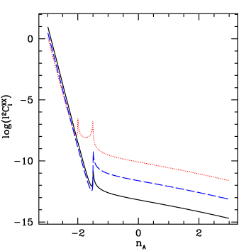
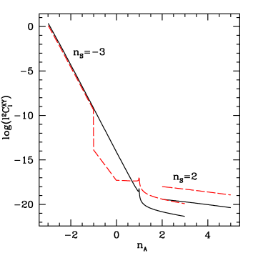
Figure 1: On the top panel we show the amplitudes of the parity even correlators, $\ell^{2}C^{(\theta\theta)}_{(A)\ell}$ (solid, black), $\ell^{2}C^{(EE)}_{(A)\ell}$ (dotted, red) and $\ell^{2}C^{(\theta E)}_{(A)\ell}$ (dashed, blue) as a function of the spectral index $n_{A}$ for $\ell=50$. The logarithm of the absolute value of $\ell^{2}C_{(A)\ell}^{(XY)}$ is shown in units of $(\Omega_{A}/\Omega_{r})^{2}\ln^{2}(z_{\rm in}/z_{\rm eq})$. We do not plot $\ell^{2}C^{(BB)}_{(A)\ell}$ which equals $\ell^{2}C^{(EE)}_{(A)\ell}$ within our approximation. The spikes at $n_{A}=-2$ for $\ell^{2}C^{(EE)}_{\ell}$ and at $n_{A}=-3/2$ are not real. They are artefacts due to the break-down of our approximations at these values.
On the bottom panel we show the corresponding parity odd correlators, $\ell^{2}C^{(\theta B)}_{(A)\ell}$ (solid, black), $\ell^{2}C^{(EB)}_{(A)\ell}$ (dashed, red) in units of $(\Omega_{A}\Omega_{S}/\Omega_{r}^{2})\ln^{2}(z_{\rm in}/z_{\rm eq})$ for $n_{S}=-2.99$ and $n_{S}=2$. In this last case, only the allowed range $n_{A}\geq n_{S}=2$ is plotted. Again the spike at $n_{A}=1$ for $n_{S}=-2.99$ and the precipitous drop at $n_{A}=-1$ in $\ell^{2}C^{(EB)}_{(A)\ell}$, are due to the limitation of our approximation close to the transition indices.

In Fig. 1, we show $\ell^{2}C_{(A)\ell}^{(XY)}$ at $\ell=50$ for the different quantities (temperature anisotropy, $E$ and $B$ polarization and correlators) as a function of $n_{A}$ with $n_{S}$ fixed to $2$ and $-2.99$. We show the absolute value of the correlator in units of

$$\ \left({\Omega_{A}\over\Omega_{r}}\right)^{2}\ln^{2}\left({z_{\rm in}\over z_{\rm eq}}\right)\simeq 10^{-10}\left({{\cal B}_{k_{D}}\over 10^{-9}{\rm Gauss}}\right)^{4}~{},$$

and

$${\Omega_{A}\Omega_{S}\over\Omega_{r}^{2}}\ln^{2}\left({z_{\rm in}\over z_{\rm eq}}\right)\simeq 10^{-10}\left({{\cal B}_{k_{D}}\over 10^{-9}{\rm Gauss}}\right)^{2}\left({B_{k_{D}}\over 10^{-9}{\rm Gauss}}\right)^{2}~{}.$$

Note that the correlators $C^{(XX)}_{A}$ and $C^{(\theta E)}_{A}$ are always negative and have to be subtracted from $C_{(S)}^{(XY)}$ which is of the same order of magnitude or larger since $\Omega_{S}\geq\Omega_{A}$ and $n_{S}\leq n_{A}$. For the limiting case, $\Omega_{S}\simeq\Omega_{A}$ and $n_{S}\simeq n_{A}$, the presence of an helical component in the magnetic field spectrum can in principle cancel the effect of the symmetric part on the CMB. In that very particular case, the signature of the presence of a magnetic field will appear only through the parity odd correlators.

From Fig. 1 it is clear that only for $n_{A,S}\lesssim-2$ and $\Omega_{A}\simeq\Omega_{S}\sim 10^{-5}$, the effect on the CMB will be of the order of a percent or more. In Ref. caprini02 it has been shown that for $n_{S}>-2$, magnetic fields with $B_{\lambda}\gtrsim 10^{-10}$Gauss over-produce gravity waves on small scales which is incompatible with the nucleosynthesis bound, for $\lambda\sim 1$ Mpc. Here we require $B_{k_{D}}\lesssim 10^{-8}$ Gauss so that $\Omega_{B}$ remains a small fraction of the radiation density throughout. Then $B_{\lambda}=B_{k_{D}}(\lambda k_{D})^{-(n+3)}\ll B_{k_{D}}$ for $n>-2$. Therefore, by keeping $B_{k_{D}}$ sufficiently small, we automatically satisfy the bound derived in Ref. caprini02 . The result is most interesting for the window of $-3<n_{S}\lesssim n_{A}\lesssim-2$ and $\Omega_{A}\simeq\Omega_{S}\sim 10^{-5}$, which requires ${\cal B}_{k_{D}}\simeq B_{k_{D}}\sim 10^{-10}$Gauss. Especially, if magnetic field helicity is causally produced which implies $n_{S}=2$ and $n_{A}=3$, this effect cannot be observed in the CMB since the parity violating terms are suppressed by about 15 orders of magnitude (see lines in the lower right corner of the bottom panel of Fig. 1).

In Fig. 2 we show the ratio $C_{(A)\ell}^{\theta B}/C_{(A)\ell}^{\theta E}$ for $n_{S}=-3$ as function of $n_{A}$. Again, we are mainly interested in the part of the graph with $-3<n_{A}<-2$, where this ratio raises from the order unity to about $10^{5}$. Hence if a close to maximal helical magnetic field, with a spectrum not too far from scale invariant, $-3<n_{S}<n_{A}<-2$ is produced in the early universe, it is more promising to search for its parity violating terms than for the parity even contributions.

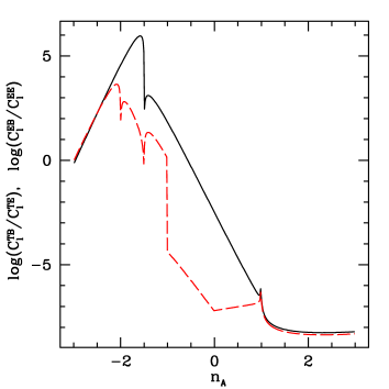
Figure 2: We show the ratio of the correlators, $C^{(\theta B)}_{\ell}/C^{(\theta E)}_{\ell}$ (solid, black), and $C^{(EB)}_{\ell}/C^{(EE)}_{\ell}$ for $n_{S}=-3$ as functions of the spectral index $n_{A}$ for $\ell=50$. The logarithm of the absolute value is shown in units of $\Omega_{A}/\Omega_{S}\leq 1$. The spikes visible at certain values of the spectral index $n_{A}$ are mainly due to our relatively crude approximations.

We can conclude that helical magnetic fields with a spectrum close to the scale invariant value, $-3<n_{S}\simeq n_{A}\lesssim-2$ and close to maximal amplitudes on small scales, $B_{k_{D}}\gtrsim 10^{-10}$ Gauss can lead to observable parity violating terms $C^{\theta B}$ and $C^{EB}$ in the CMB. Such magnetic fields might in principle be produced during some inflationary epoch where the photon is not minimally coupled or via its coupling to the dilaton (see inflat ; stringcos for various proposal of magnetic field production during an inflationary phase). However, so far no concrete proposal has led to $n_{S,A}\simeq-3$, nor to the creation of a helical term. As we have shown, the effect is largely suppressed and clearly unobservable for causally produced magnetic fields, e.g. , during the electroweak phase transition or even later.

Nevertheless, our calculation also demonstrates the effect of parity violating processes during inflation which may lead to a non-vanishing helical component of gravity waves, ${\cal H}\neq 0$, see Eq. (61). In this case the above calculation can be trivially repeated and will result in non-vanishing parity violating CMB correlators, $C^{\theta B}\neq 0$ and $C^{EB}\neq 0$. We think that already this remark, together with our knowledge that at least at low energies, nature does violate parity, should be sufficient motivation to derive experimental limits on these correlators.

Appendix A The source for gravity waves

In this appendix we present some details on how to compute the gravity waves source functions $f(k)$ and $g(k)$. The first step is to evaluate the two point correlator of the magnetic field stress-energy tensor (25): using Wick’s theorem (26) and definition (1), after a longish but simple calculation we obtain

$$\langle\tau_{ij}({\mathbf{k}})\tau^{*}_{lm}({\mathbf{k}^{\prime}})\rangle = \frac{1}{4}{1\over(4\pi)^{2}}\delta({\mathbf{k}}-{\mathbf{k}}^{\prime})\int d^{3}p\left(\right.S(p)S(|{\mathbf{k}}-{\mathbf{p}}|)[(\delta_{il}-\hat{p}_{i}\hat{p}_{l})(\delta_{jm}-(\widehat{{\mathbf{k}}-{\mathbf{p}}})_{j}(\widehat{{\mathbf{k}}-{\mathbf{p}}})_{m})$$ (113)

$$+(\delta_{im}-\hat{p}_{i}\hat{p}_{m})(\delta_{jl}-(\widehat{{\mathbf{k}}-{\mathbf{p}}})_{j}(\widehat{{\mathbf{k}}-{\mathbf{p}}})_{l})]$$

$$-A(p)A(|{\mathbf{k}}-{\mathbf{p}}|)[\epsilon_{ilt}\epsilon_{jmr}{\hat{p}}_{t}(\widehat{{\mathbf{k}}-{\mathbf{p}}})_{r}+\epsilon_{imf}\epsilon_{jlg}{\hat{p}}_{f}(\widehat{{\mathbf{k}}-{\mathbf{p}}})_{g}]$$

$$+iS(p)A(|{\mathbf{k}}-{\mathbf{p}}|)[\epsilon_{jmr}(\delta_{il}-{\hat{p}}_{i}{\hat{p}}_{l})(\widehat{{\mathbf{k}}-{\mathbf{p}}})_{r}+\epsilon_{jlg}(\delta_{im}-{\hat{p}}_{i}{\hat{p}}_{m})(\widehat{{\mathbf{k}}-{\mathbf{p}}})_{g}]$$

$$+iA(p)S(|{\mathbf{k}}-{\mathbf{p}}|)[\epsilon_{ilt}(\delta_{jm}-{\widehat{\bf(k-p)}}_{j}{\widehat{\bf(k-p)}}_{m}){\hat{p}}_{t}+\epsilon_{imf}(\delta_{jl}-{\widehat{\bf(k-p)}}_{j}{\widehat{\bf(k-p)}}_{l}){\hat{p}}_{f}]\left.\right\}$$

$$+\cdots\delta_{ij}+\cdots\delta_{lm}~{}.$$

The isotropic tensor spectrum in the case of a magnetic field spectrum without helicity term is derived in durrer00 . Here we concentrate on the source terms which contain the helical part of the magnetic field spectrum.

By acting with tensor projector on (113), we find expressions (37) and (38) for the symmetric and helical parts of the source spectrum. Taking into account that the angle $\beta={\hat{\mathbf{k}}}\cdot(\widehat{{\bf k-p}})={{k-p\gamma}\over{\sqrt{k^{2}-2kp\gamma+p^{2}}}}$, we can rewrite the two expressions which contain $A(k)$ in the form

$$f^{A}(k) = {8\over(4\pi)^{5}}\int d^{3}pA(p)A(|{\mathbf{k}}-{\mathbf{p}}|){{\gamma\cdot(k-p\gamma)}\over{\sqrt{k^{2}-2kp\gamma+p^{2}}}}$$ (114)

$$g(k) = {4\over(4\pi)^{5}}\int d^{3}p\left[S(p)A(|{\mathbf{k}}-{\mathbf{p}}|){(k-p\gamma)(1+\gamma^{2})\over\sqrt{k^{2}-2kp\gamma+p^{2}}}+A(p)S(|{\mathbf{k}}-{\mathbf{p}}|)\left(2\gamma-{\gamma p^{2}(1-\gamma^{2})\over k^{2}-2kp\gamma+p^{2}}\right)\right]~{}.$$ (115)

The contribution to $f(k)$ from $S$ alone is computed in Ref.  durrer00 . There one finds

$$f^{S}(k)={2\over(4\pi)^{5}}\int d^{3}pS(p)S(|{\mathbf{k}}-{\mathbf{p}}|)(1+\gamma^{2})\left(1+{(k-p\gamma)^{2}\over k^{2}-2kp\gamma+p^{2}}\right)~{}.$$ (116)

We can now substitute the power law Ansatz  (II,11) for $S$ and $A$ in these expressions and try to calculate the integrals. The integration over $\gamma={\hat{\mathbf{k}}}\cdot{\hat{\mathbf{p}}}$ is elementary, using

$$\int d\gamma\,(k^{2}+p^{2}-2kp\gamma)^{\alpha\over 2} = -\frac{1}{kp(\alpha+2)}(k^{2}+p^{2}-2kp\gamma)^{\alpha+2\over 2}$$

$$\int d\gamma\,\gamma^{m}\,(k^{2}+p^{2}-2kp\gamma)^{\alpha\over 2} = -\frac{\gamma^{m}}{kp(\alpha+2)}(k^{2}+p^{2}-2kp\gamma)^{\alpha+2\over 2}+\frac{m}{kp(\alpha+2)}\int d\gamma\,\gamma^{m-1}\,(k^{2}+p^{2}-2kp\gamma)^{\alpha+2\over 2}~{}.$$ (117)

This last integration by parts has to be performed in the worst cases three times, reducing the power $m$ of $\gamma$ from $3$ down to $0$.

Since we are integrating $\gamma$ over the interval $[-1,1]$, we get a series of $m+1$ terms of the form

$${(k+p)^{\alpha+2n}\pm|k-p|^{\alpha+2n}\over(k\,p)^{n}}~{},$$ (118)

with $n=1,2,...(m+1)$. To evaluate the integral over $p$, we can expand those terms using the binomial decomposition $(1+x)^{\alpha}=1+\alpha x+\alpha(\alpha-1)x^{2}+\cdots$. Since, in general, the value of the exponent $\alpha$ is not an integer, we need to truncate the series somewhere, which is well justified only if $x\ll 1$. To achieve this, we split the integral into two contributions, $\int_{0}^{k_{D}}=\int_{0}^{k}+\int_{k}^{k_{D}}$. In the first term $p/k<1$, while in the second $k/p<1$, which allows us to approximate Eq. (118) truncating the binomial series at the second term,

$$(k+p)^{\alpha}-|k-p|^{\alpha}\simeq\cases{2\alpha k^{\alpha-1}p+{1\over 3}\alpha(\alpha-1)(\alpha-2)k^{\alpha-3}p^{3}&$p<k$\cr 2\alpha p^{\alpha-1}k+{1\over 3}\alpha(\alpha-1)(\alpha-2)p^{\alpha-3}k^{3}&$p>k$\cr}$$ (119)

and

$$(k+p)^{\alpha}+|k-p|^{\alpha}\simeq\cases{2k^{\alpha}+\alpha(\alpha-1)k^{\alpha-2}p^{2}&$p<k$\cr 2p^{\alpha}+\alpha(\alpha-1)p^{\alpha-2}k^{2}&$p>k$ ~{}.\cr}$$ (120)

We then perform the integration over $p$. For each contribution we keep only the terms which, depending on the value of the spectral index, may dominate the result. So, we finally obtain, for $k<k_{D}$

$$f(k) \simeq \frac{\lambda^{3}}{2(2n_{S}+3)}\left[\frac{B^{2}_{\lambda}}{2\Gamma\left(\frac{n_{S}+3}{2}\right)}\right]^{2}\left((\lambda k)^{2n_{S}+3}_{D}+\frac{n_{S}}{n_{S}+3}(\lambda k)^{2n_{S}+3}\right)-$$ (121)

$$\mbox{}-\frac{2\lambda^{3}}{3(2n_{A}+3)}\left[\frac{{\cal B}^{2}_{\lambda}}{2\Gamma\left(\frac{n_{A}+4}{2}\right)}\right]^{2}\left((\lambda k)^{2n_{A}+3}_{D}+\frac{n_{A}-1}{n_{A}+4}(\lambda k)^{2n_{A}+3}\right)$$

$$\simeq {\mathcal{A}}_{S}\lambda^{2n_{S}+3}\left(k^{2n_{S}+3}_{D}+\frac{n_{S}}{n_{S}+3}\,k^{2n_{S}+3}\right)-{\cal A}_{A}\lambda^{2n_{A}+3}\left(k^{2n_{A}+3}_{D}+\frac{n_{A}-1}{n_{A}+4}\,k^{2n_{A}+3}\right)$$ (122)

$$g(k) \simeq \frac{4}{3}\frac{\lambda^{4}k}{(n_{S}+n_{A}+2)}\left[\frac{B^{2}_{\lambda}}{2\Gamma\left(\frac{n_{S}+3}{2}\right)}\right]\left[\frac{{\mathcal{B}}^{2}_{\lambda}}{2\Gamma\left(\frac{n_{A}+4}{2}\right)}\right]\left((\lambda k_{D})^{n_{S}+n_{A}+2}+\frac{n_{A}-1}{n_{S}+3}(\lambda k)^{n_{S}+n_{A}+2}\right)$$ (123)

$$\simeq {\cal C}k\lambda\,(\lambda k_{D})^{n_{S}+n_{A}+2}\,\left[1+\frac{n_{A}-1}{n_{S}+3}\left(\frac{k}{k_{D}}\right)^{n_{S}+n_{A}+2}\right]~{},$$ (124)

where the coefficients are given by the magnetic field amplitudes at scale $\lambda$:

$${\cal A}_{S} \simeq \frac{\lambda^{3}}{2(2n_{S}+3)}\left[\frac{B^{2}_{\lambda}}{2\Gamma\left(\frac{n_{S}+3}{2}\right)}\right]^{2}$$ (125)

$${\cal A}_{A} \simeq \frac{2\lambda^{3}}{3(2n_{A}+3)}\left[\frac{{\mathcal{B}}^{2}_{\lambda}}{2\Gamma\left(\frac{n_{A}+4}{2}\right)}\right]^{2}$$ (126)

$${\cal C} \simeq \frac{4}{3}\frac{\lambda^{3}}{(n_{S}+n_{A}+2)}\left[\frac{B^{2}_{\lambda}}{2\Gamma\left(\frac{n_{S}+3}{2}\right)}\right]\left[\frac{{\mathcal{B}}^{2}_{\lambda}}{2\Gamma\left(\frac{n_{A}+4}{2}\right)}\right]~{}.$$ (127)

The first part of $f(k)$, which is the contribution from the symmetric part of the magnetic field power spectrum, has been taken from durrer00 ; mack02 . The singularities at $n_{S},~{}n_{A}=-3/2$ respectively and at $n_{S}+n_{A}=-2$ are removable.

Appendix B useful mathematical relations

B.1 Integrals of Bessel functions

In Section V, we use approximate solutions for the three integrals

$$\int^{x_{0}}_{x_{\text{dec}}}dx\,\frac{j_{2}(x)}{x}\frac{j_{\ell}(x_{0}-x)}{(x_{0}-x)^{2}}~{},~{}~{}~{}~{}~{}~{}~{}~{}~{}~{}\int^{x_{0}}_{x_{\text{dec}}}dx\,\frac{j_{2}(x)}{x}\frac{j_{\ell}(x_{0}-x)}{(x_{0}-x)}~{},~{}~{}~{}~{}~{}~{}~{}~{}~{}~{}\int^{x_{0}}_{x_{\text{dec}}}dx\,\frac{j_{2}(x)}{x}j_{\ell}(x_{0}-x)~{}.$$ (128)

These integrals are solvable only by numerical method. However, the aim of this paper is to give an approximate analytic result. In this appendix we therefore derive and test analytic approximations to the above integrals. To achieve this, we first modify them slightly, in order to make them solvable analytically. Then, we adjust the result obtained in this way by comparing it with the exact numerical integration.

Let us concentrate, as an example, on the first integral. We first perform a variable transform to $y=x_{0}-x$. The integration boundaries then become $0$ and $x_{0}-x_{\text{dec}}$. Below, we derive an approximation for

$$\int_{0}^{x_{0}}\frac{j_{2}(x_{0}-y)}{x_{0}-y}\frac{j_{\ell}(y)}{y^{n}}dy$$

Since Bessel functions change on a scale $\Delta y\sim 1$, this approximation is good for the integrals in Eq. (128) if $x_{\text{dec}}<1$. After the integration over x in Eq.(128) we have to perform an integration over $k$. For $\ell$ fixed, this integral is either dominated by the contribution art $k\eta_{0}=x_{0}=\ell$ or at the upper cutoff, $k_{D}$. For the integrals which are dominated at $x_{0}=k\eta_{0}\sim\ell$, the inequality $x_{\text{dec}}<1$ is equivalent to $\ell\simeq x_{0}\simeq 60x_{\text{dec}}\lesssim 60$. In some cases, however, our integral over $k$ is dominated at the upper cutoff $k_{D}$ with $\eta_{\text{dec}}k_{D}\gg 60$ and of course also $\eta_{0}k_{D}\gg 60$. Since for $\ell\simeq 60$, the dominant contribution to the integral comes from $y\lesssim 60$, our inaccuracy of the boundary will not invalidate the approximation also for this case.

The approximation in the upper boundary of the integral, $x_{0}-x_{\text{dec}}\simeq x_{0}$ makes us miss the characteristic decay of fluctuations on angular scales corresponding to $\ell\gtrsim 60$.

To make the first integral in Eq. (128) solvable analytically, we now modify the powers of $y$ and $x_{0}-y$. Taking into account that the spherical Bessel Function $j_{\nu}(x)$ has its maximum value at $x\simeq\nu$, we make the attempt:

$$\int^{x_{0}}_{0}dx\,\frac{j_{2}(x)}{x}\frac{j_{\ell}(x_{0}-x)}{(x_{0}-x)^{2}} = \frac{\pi}{2}\int^{x_{0}}_{0}dx\,\frac{J_{5/2}(x)}{x^{3/2}}\frac{J_{\ell+{1\over 2}}(x_{0}-x)}{(x_{0}-x)^{5/2}}$$ (129)

$$\simeq \frac{\pi}{2}\sqrt{\frac{2}{5\,\ell}}\int^{x_{0}}_{0}dx\,\frac{J_{5/2}(x_{0}-y)}{x_{0}-y}\frac{J_{\ell+{1\over 2}}(y)}{y^{2}}~{}.$$

$$\simeq {\pi\over 5}\sqrt{\frac{2}{5\,\ell}}{J_{\ell+3}(x_{0})\over x_{0}^{2}}~{}.$$ (130)

For the last equality, we have used 6.581.2 of gradshteyn94  ,

$$\int^{a}_{0}dx\,x^{b-1}(a-x)^{-1}J_{p}(x)J_{q}(a-x) = \frac{2^{b}}{aq}\sum^{\infty}_{m=0}\frac{(-1)^{m}\,\Gamma(b+p+m)\,\Gamma(b+m)}{m!\,\Gamma(b)\,\Gamma(p+m+1)}\,(b+p+q+2m)\,J_{b+p+q+2m}(a)~{},$$ (131)

$$\mbox{}(\text{Re}\,(b+p)>0,\,\text{Re}\,q>0)$$

and the recurrence relation $J_{\nu-1}(x)+J_{\nu+1}(x)=\frac{2\nu}{x}J_{\nu}$ (9.1.27 of abramowitz72 ), keeping only the highest order terms in $\ell$. We can now compare this approximated analytic result with an exact numerical integration. Since the analytic result is again a Bessel function divided by a power law, it has a maximum at $x_{0}\simeq\ell$, and its envelope has a power law decay for $x_{0}>\ell$. This two characteristics are very well reproduced by the numerical result, which however decays somewhat faster; it turns out that a better approximation is

$$\int^{x_{0}}_{0}dx\,\frac{j_{2}(x)}{x}\frac{j_{\ell}(x_{0}-x)}{(x_{0}-x)^{2}}\simeq\frac{1}{3}\sqrt{\frac{3\,\ell}{2}}\,\frac{J_{\ell+3}(x_{0})}{x_{0}^{3}}~{}.$$ (132)

To estimate the goodness of our approximation, let us now take into account the integration over $k$, as in Eq. (67). What we are finally interested in is (Eq. (75))

$$\int_{0}^{x_{D}}dx_{0}\,x_{0}^{2}\,{J^{2}_{\ell+3}(x_{0})\over x_{0}^{6}}\left[1+\frac{n_{A}-1}{n_{A}+4}\,\left({x_{0}\over x_{D}}\right)^{2n_{A}+3}\right]~{}.$$ (133)

As already discussed in the main text, this integral is always convergent and dominated by the contribution around $x_{0}\simeq\ell$ : we should therefore make sure that our approximation is good around that value. We have that for $\ell=30$, our approximation underestimates the numerical result by about factor of two; for $\ell=40$, the error reduces to $15\%$, and is always smaller for larger values of $\ell$.

Fig. 3 shows the numerical result for the integral in (132) (green, dotted line), together with its analytical approximation (the right hand side of Eq. (132), blue and long dashed) and a numerical evaluation of the same integral when $x_{\rm dec}$ is not set to zero (red, solid). For small values of $\ell$ (in the left hand panel of Fig. 3, $\ell=50$), Eq. (132) is a good approximation in the region $x_{0}\simeq\ell$. However, if $\ell>60$ setting $x_{\rm dec}\rightarrow 0$ causes a large overestimation of the result. In the right hand panel of Fig. 3 it is shown that, for $\ell=100$, the difference between the integral with lower bound $0$ and the one with lower bound $x_{\rm dec}$ is of more than a factor of ten. Consequently, as already stated before, we can rely on all our approximations only for $\ell\lesssim 60$.

We proceed now to evaluate integral (133). Since $x_{D}=k_{D}\eta_{0}\gtrsim 10^{6}$, for $\ell\lesssim 60$, integral (133) can be calculated in the limit $x_{D}\rightarrow\infty$, using formula 6.574.2 of gradshteyn94 :

$$\int^{\infty}_{0}dx\,J_{p}(x)J_{q}(x)x^{-b} = \frac{\Gamma(b)\Gamma\left(\frac{p+q-b+1}{2}\right)}{2^{b}\Gamma\left(\frac{-p+q+b+1}{2}\right)\Gamma\left(\frac{p+q+b+1}{2}\right)\Gamma\left(\frac{p-q+b+1}{2}\right)}$$

$$\mbox{}(\text{Re}\,(p+q+1)>\text{Re}\,b>0)~{}.$$

This approximation is used for example in Eqs. (V.1, V.1).

With the same procedure we can approximate the second integral of Eq. (128), for which we find ($\ell\lesssim 60$)

$$\int^{x_{0}}_{x_{\rm dec}}dx\,\frac{j_{2}(x)}{x}\frac{j_{\ell}(x_{0}-x)}{(x_{0}-x)}\simeq\frac{1}{3}\sqrt{\frac{3\,\ell}{2}}\frac{J_{\ell+3}(x_{0})}{x_{0}^{2}}~{}.$$ (135)

This approximation underestimates the numerical result with an error of about $40\%$ for $\ell=30$, which reduces to $20\%$ at $\ell=60$. In this case also, the integral over $x_{0}$ is convergent, and we can proceed as before.

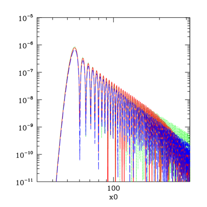
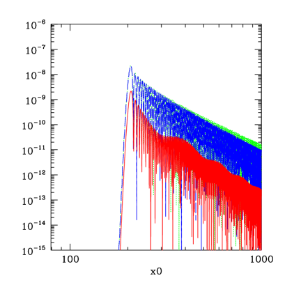
Figure 3: In both panels, as a function of $x_{0}$: the green dotted line shows the numerical value of the integral in (132), the blue, long dashed line shows the analytic approximation (right hand side of Eq. (132)), and the red, solid line shows the numerical value of integral (132) if $x_{\rm dec}$ is not put to zero. All these functions are squared, and multiplied by $x_{0}^{3}$: this gives us an indication of the result, after the integration over $x_{0}$, as stated in Eq. (133). In the left panel $\ell=50$, in the right panel $\ell=200$. First of all, we note that it appears clearly that the value of the integrals is dominated at $x_{0}\simeq\ell$, and that the function goes to zero quicker than $x_{0}^{-3}$, which justifies our approximation $x_{D}\rightarrow\infty$ and the use of formula B.1. Secondly, we note that for $\ell=50$ and $x_{0}\sim\ell$, our approximation (blue, long-dashed) is good for both the integrals. However, if $\ell=200$, the approximation overestimate the correct numerical result by about a factor of ten.

The situation is different for the third integral of Eq. (128). In this case, the numerical result is approximated by the following function ($\ell\lesssim 60$):

$$\int^{x_{0}}_{x_{\rm dec}}dx\,\frac{j_{2}(x)}{x}j_{\ell}(x_{0}-x)\simeq\frac{1}{3}\sqrt{\frac{2}{5}}\,\frac{J_{\ell+3}(x_{0})}{\sqrt{x_{0}}}~{}.$$ (136)

It is clear that if we insert this function in an integral like (133) we cannot perform the limit $x_{D}\rightarrow\infty$ since this integral is dominated at the upper cutoff. Consequently, we need a good approximation for the behavior of the integral for large values of $x_{0}\rightarrow x_{D}$. In this case, we no longer require our approximation to be accurate at $x_{0}\simeq\ell$, but we concentrate on its behavior for high values of $x_{0}$, which will dominate in the integral over $x_{0}$. Fig. 4 shows the approximation for $\ell=30$, which overestimate the numerical result by an error within $1\%$.

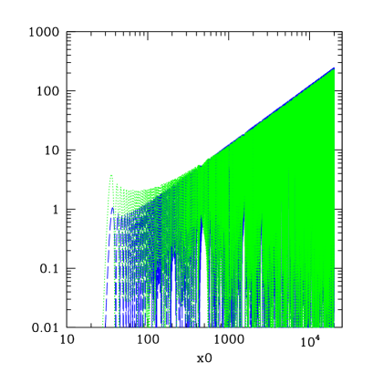
Figure 4: We plot the value of integral (136) squared and multiplied by $x_{0}^{3}$ as function of $x_{0}$, for $\ell=30$. The green, dotted line represents again the numerical result ($x_{\rm dec}\rightarrow 0$), and the blue, long dashed line is the analytic approximation. In this case the slope is positive, and hence the integral $dx_{0}/x_{0}$ of this function is dominated by the upper cutoff.

We also have to evaluate the integral over $x_{0}^{2}\,dx_{0}$ of the square of (136), which we encounter in two different cases. The first (see Section V.2) is of the kind $\int^{x_{D}}_{0}dx\,x^{p}J^{2}_{\ell}(x)$. For $p<0$ this integral converges and we may evaluate it in the limit $x_{D}\rightarrow\infty$, in which it is of the form (131). For $p>0$ and $x_{D}\gg\ell^{2}$, the integral can be approximated using the asymptotic expansion of $J_{\ell}(x)$ for large arguments abramowitz72 , $J_{\ell}(x)\sim\sqrt{2/(\pi x)}\cos[x-(2\ell+1)\pi/4]$. Approximating the oscillations by a factor of $1/2$, we obtain

$$\int^{x_{D}}_{0}dx\,x^{p}J^{2}_{\ell}(x)\simeq\int^{x_{D}}_{\ell^{2}}dx\,x^{p}J^{2}_{\ell}(x)\simeq\cases{\frac{x^{p}_{D}}{p\pi},&$p>0$\cr\frac{1}{\pi}\ln\left(\frac{x_{D}}{\ell^{2}}\right),&$p=0$~{}.\cr}$$ (137)

For the second case, $\int_{0}^{x_{D}}dx\,x^{p}J_{\ell}(x)J_{\ell+1}(x)$, which we encounter in Section VI, we use again the large argument approximation for the Bessel functions, for $x\gg\ell^{2}$,

$$J_{\ell}(x)J_{\ell+1}(x) \simeq {2\over\pi x}\cos\left(x-(2\ell+1){\pi\over 4}\right)\cos\left(x-(2\ell+3){\pi\over 4}\right)={2\over\pi x}\cos\left(x-(2\ell+1){\pi\over 4}\right)\sin\left(x-(2\ell+1){\pi\over 4}\right)$$ (138)

$$= {1\over\pi x}\sin\left(2x-\left(\ell+{1\over 2}\right)\pi\right)={(-1)^{\ell+1}\over\pi x}\cos(2x)~{},$$

so that for $p>0$

$$\int_{0}^{x_{D}}dx\,x^{p}J_{\ell}(x)J_{\ell+1}(x)\simeq{(-1)^{\ell+1}\over\pi}\int^{x_{D}}_{\ell^{2}}dx\,x^{p-1}\cos\left(2x\right)\simeq{(-1)^{\ell+1}\over 2\pi}\left(x_{D}^{p-1}\sin(2x_{D})-\ell^{2p-2}\sin(2\ell^{2})\right)~{}.$$ (139)

In the limits to which we have restricted ourselves, we always have $x_{D}\gg\ell^{2}$. Consequently, the dominant contribution in the last expression can be given either by the first term in the bracket, if $p>1$, or by the second term, if $p<1$. Numerical checks show that the approximation is good for $p>1$, but it is rather poor in the second case, $p<1$. Since we shall not be very much interested in this case, we do not go any further in this work.

When evaluating expression (B.1), we often also use

$$\Gamma(2x) = \frac{2^{2x-1}}{\sqrt{\pi}}\Gamma(x)\Gamma\left(x+\frac{1}{2}\right)$$

$$\frac{\Gamma(x+a)}{\Gamma(x+b)} \sim x^{a-b}+\mathcal{O}(x^{a-b-1})\>\>\>\>\>\>\>\mbox{for $x\gg 1$}$$ (140)

(see Eqs. (6.1.18) and (6.1.47) of abramowitz72 ).

B.2 Recurrent Relations for spherical Bessel Functions

We use several recurrence relations for spherical Bessel functions in our derivations, most notably

$$\frac{\ell+1}{x}j_{\ell}(x)+j^{\prime}_{\ell}(x)=j_{\ell-1}(x)$$ (141)

and

$$\frac{\ell}{x}j_{\ell}(x)-j^{\prime}_{\ell}(x)=j_{\ell+1}(x)~{}.$$ (142)

References

(1) T. Vachaspati, Phys. Rev. Lett. 87
251302 (2001).
(2) A. Brandenburg, and E. Blackman,
astro-ph/0212019.
(3) K. Jedamzik, V. Katalinić, and A.V. Olinto,
Phys. Rev. D 57, 3264 (1998).
(4) R. Durrer, P.G. Ferreira, and T. Kahniashvili,
Phys. Rev. D 61, 043001 (2000).
(5) D. Grasso and H.R. Rubinstein,
Phys. Rep. 348, 163 (2001).
(6) A. Mack, T. Kahniashvili, and A. Kosowsky,
Phys. Rev. D 65, 123004 (2002).
(7) L. Pogosian, T. Vachaspati, S. Winitzki,
Phys. Rev. D 65, 3264 (2002).
(8) J. Ahonen and K. Enqvist,
Phys. Lett. B 382, 40 (1996).
(9) K. Subramanian and J.D. Barrow,
Phys. Rev. Lett. 81, 3575 (1998).
(10) K. Subramanian and J.D. Barrow,
Phys. Rev. D 58, 083502 (1998).
(11) W. Hu and M. White,
Phys. Rev. D 56, 596 (1997).
(12) C. Caprini and R. Durrer,
Phys. Rev. D 65, 023517 (2002).
(13)R. Durrer and C. Caprini, JCAP in print (2003)
[astro-ph/0305059 ].
(14) J.D. Jackson, Classical Electrodynamics
(Wiley, New York, 1975).
(15) R. Durrer and M. Kunz, Phys. Rev. D 57, R3199
(1998).
(16) D.N. Spergel et al, astro-ph/0302209.
(17)M. Christensson, M. Hindmarsh and
A. Brandenburg, Phys. Rev. E 64, 056405 (2001).
(18) R. Durrer and T. Kahniashvili,
Helv. Phys. Acta, 71, 445 (1998).
(19) M. Abramowitz and I. Stegun,
Handbook of Mathematical Functions, Dover, New York (1972).
(20) R. Durrer, Fundam. Cosm. Phys. 15, 209 (1994).
(21) M. Zaldarriaga and U. Seljak,
Phys. Rev. D 55, 1830 (1997).
(22) M. Kamionkowski, A. Kosowsky, and
A. Stebbins, Phys. Rev. D 55, 7368 (1997).
(23) A. Kosowsky and A. Loeb,
Astrophys. J. 469, 1 (1996).
(24)M.S.Turner and L.M. Widrow, Phys. Rev. D 37,
2743 (1988);
B. Ratra, Astrophys. J. Lett. 391 L1 (1992);
W.D.Garretson, G.B. Field and S.M.Carroll, Phys. Rev. D
46 5346 (1992);
O.Bertolami and D.F.Mota, Phys. Lett. B 455, 96 (1999);
A. Davis, K. Dimopoulos, T. Prokopec and O. Törnkvist,
Phys. Lett. B501, 165 (2001).
(25) M. Gasperini, M. Giovannini and G. Veneziano,
Phys. Rev. Lett. 75, 3796 (1995);
D. Lemoine and M. Lemoine, Phys. Rev. D 52, 1955 (1995).
(26) I.S. Gradshteyn and I.M. Ryzhik,
Table of Integrals, Series, and Products, Academic Press, New
York and London (1965).