Modelling the two point correlation function of galaxy clusters in the Sloan Digital Sky Survey

Abstract

We study the clustering properties of the recently compiled SDSS cluster catalog using the two point correlation function in redshift space. We divide the total SDSS sample into two richness subsamples, roughly corresponding to Abell $R\geq 0$ and APM clusters, respectively. If the two point correlations are modeled as a power law, $\xi(r)=(r_{\circ}/r)^{\gamma}$, then the best-fitting parameters for the two subsamples are $r_{\circ}=20.7^{+4.0}_{-3.8}\;h^{-1}$ Mpc with $\gamma=1.6^{+0.4}_{-0.4}$ and $r_{\circ}=9.7^{+1.2}_{-1.2}$ with $\gamma=2.0^{+0.7}_{-0.5}\;h^{-1}$ Mpc, respectively. Our results are consistent with the dependence of cluster richness to the cluster correlation length.

Finally, comparing the SDSS cluster correlation function with that predictions from three flat cosmological models ($\Omega_{\rm m}=0.3$) with dark energy (quintessence), we estimate the cluster redshift space distortion parameter $\beta\simeq\Omega_{\rm m}^{0.6}/b_{\circ}$ and the cluster bias at the present time. For the $\Lambda$CDM case we find $\beta=0.2^{+0.029}_{-0.016}$, which is in agreement with the results based on the large scale cluster motions.

Keywords: galaxies: clusters: general - cosmology: theory - large-scale structure of universe

1 Introduction

Galaxy clusters occupy a special position in the hierarchy of cosmic structure formation, being the largest gravitationally collapsed objects in the universe. Therefore, they appear to be ideal tools for testing theories of structure formation as well as studying large-scale structure. The traditional indicator of clustering, the cluster two-point correlation function, is a fundamental statistical test for the study of the cluster distribution and is relatively straightforward to measure from observational data.

Indeed, many authors based on optical and X-ray data have shown that the large scale clustering pattern of galaxy clusters is well described by a power law, $\xi(r)=(r_{\circ}/r)^{\gamma}$, with $\gamma=1.6-2$. The correlation length $r_{\circ}$ lies in the interval $r_{\circ}=13-25h^{-1}$Mpc, depending on the cluster richness as well as the analyzed sample (cf. Bahcall & Soneira 1983; Klypin & Kopylov 1983; Lahav et al. 1989; Bahcall & West 1992; Peacock & West 1992; Dalton et al. 1994; Nichol, Briel & Henry 1994; Croft et al. 1997; Abadi, Lambas & Muriel 1998; Borgani, Plionis & Kolokotronis 1999; Collins et al. 2000; Tago et al. 2002; Moscardini, Matarrese & Mo 2001; Gonzalez, Zaritsky & Wechsler 2002). However, a serious issue here is how the galaxy clusters trace the underlying mass distribution. The cluster distribution traces scales that have not yet undergone the non-linear phase of gravitationally clustering and thus simplifying their connection to the initial conditions of cosmic structure formation. Galaxy clusters is strong biased with respect to the matter distribution (e.g. Peacock & Dodds 1994 and references therein).

In this paper we utilize the recently completed SDSS CE cluster catalog (Goto et al. 2002) in order: (i) to study the two point correlation function in redshift space and (ii) to calculate the relative cluster bias at the present time comparing the observational results with those derived from three flat cosmological models with dark energy (quintessence). The structure of the paper is as follows. The observed dataset and its measured correlation function are presented in section 2. In section 3 we give a brief account of the method used to estimate the predicted correlation function in different CDM spatially flat cosmologies. The linear growth rate of clustering in quintessence cosmological models can be found in section 4, while in section 5 we fit the SDSS cluster clustering to different cosmological and biasing models. Finally, we draw our conclusions in section 6.

2 Estimation of the SDSS cluster correlation function

2.1 Cluster catalogue

In this work we use the recent SDSS CE cluster catalog (Goto et al. 2002), which contains 2770 and 1868 galaxy clusters in the North ($145.1^{\circ}<\alpha<236.0^{\circ}$, $-1.25^{\circ}<\delta<1.25^{\circ}$) and South ($350.5^{\circ}<\alpha<56.61^{\circ}$, $-1.25^{\circ}<\delta<1.25^{\circ}$) slices respectively, covering an area of $\sim 400$deg² in the sky. Redshifts are converted to proper distances using a spatially flat cosmology with $H_{\circ}=100h\,$km s${}^{-1}\,$Mpc^-1 and $\Omega_{\rm m}=0.3$. The cluster redshifts are estimated using the color information by identifying the bin in $g-r$ which has the largest number of galaxies around the color prediction of elliptical galaxies (Fukugita, Shimasaku, Ichikawa 1995) at different redshifts (which define the different $g-r$ bins). Due to the fact that the true and estimated redshifts are better correlated for $z<0.3$ (Goto et al. 2002), we will limit our analysis within this redshift range, corresponding to a limiting distance of $r_{\rm max}\leq 836h^{-1}\,$Mpc.

In Fig. 1, we present the estimated (histogram) and the expected for a volume limited sample (solid line), number of the SDSS clusters as a function of redshift. It is evident that the number of SDSS clusters appears to follow the equal-volume $\propto r^{3}$ law out to $z\sim 0.23$, a fact corroborated also from the standard Kolmogorov-Smirnov (KS) test which gives probability of consistency between model and observations (up to $z\leq 0.23$) of ${\cal P}_{\rm KS}\simeq 0.43$. Therefore, this SDSS cluster sample is the only to-date sample that is volume limited to such a large distance and can thus play an important role in large scale structure studies.

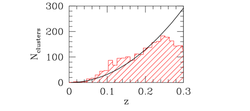
Figure 1: The estimated (histogram) and the expected (line) number of the SDSS clusters as a function of redshift.

We apply the cluster correlation function analysis using clusters of two richness class: (a) $N_{\rm gal}\geq 30$ members (roughly corresponding to Abell $R\geq 0$; hereafter $S_{1}$ sample) and (b) $N_{\rm gal}\geq 20$ members (roughly corresponding to APM clusters; hereafter $S_{2}$ sample). These two subsamples contains 200 and 524 entries with corresponding mean densities of $n_{\rm S_{1}}(\leq z_{\rm max})\simeq 8.42(\pm 0.06)\times 10^{-6}h^{3}\,$Mpc^-3 and $n_{\rm S_{2}}(\leq z_{\rm max})\simeq 2.20(\pm 0.10)\times 10^{-5}h^{3}\,$Mpc^-3, giving rise to inter-cluster separations of the order of $d_{\rm S_{1}}\sim 49.15\pm 2.56$ $h^{-1}$Mpc and $d_{\rm S_{2}}\sim 35.66\pm 2.18$ $h^{-1}$Mpc, respectively.

2.2 SDSS cluster correlations

We estimate the redshift space correlation function using the estimator described by Hamilton (1993):

$$\xi_{\rm S_{j}}(r)=4\frac{N_{DD}\langle N_{RR}\rangle}{\langle N_{DR}\rangle^{2}}-1$$ (1)

where $j=1,2$ and $N_{DD}$ is the number of cluster pairs in the interval $[r-\Delta r,r+\Delta r]$. While, $\langle N_{RR}\rangle$ and $\langle N_{DR}\rangle$ is the average, over 10000 random simulations with the same properties as the real data (boundaries and redshift selection function), cluster-random and random-random pairs, respectively. The random catalogues were constructed by randomly reshuffling the angular coordinates of the clusters (within the limits of the catalogue), while keeping the same redshifts and thus exactly the same redshift selection function as the real data.

Note that in order to take into account the possible systematic effects (eg. fraction of high-$z$ clusters missed by the finding algorithm due to SDSS magnitude limit) in the different cluster subsamples we generate random catalogs, utilized the individual distance distribution of each subsample and not the overall SDSS cluster selection function. We compute the errors on $\xi_{\rm S_{j}}(r)$ from 100 bootstrap re-samplings of the data (Mo, Jing & B$\ddot{\rm o}$rner 1992).

Figure 2: The spatial two-point correlation function (points) in redshift space for the $\rm S_{1}$ (Abell R=0 richness-right panel) and $\rm S_{2}$ (APM richness-left panel) samples. The error bars are estimated using the bootstrap procedure. The dashed lines represent the best-fitting power low $\xi_{\rm S_{j}}(r)=(r_{\circ}/r)^{\gamma}$ (see parameters in table 1).

Table 1: Results of the correlation function analysis for clusters of the two richness class (${\rm S}_{1}$ and $\rm S_{2}$ samples). Errors of the fitted parameters represent $2\sigma$ uncertainties. Finally, the $r_{\circ}$ has units of $h^{-1}\,$Mpc.

Sample	No. of clusters	$r_{\circ}$	$\gamma$	$r_{\circ}(\gamma=1.8)$
$\rm S_{1}$	200	$20.7^{+4.0}_{-3.8}$	$\gamma=1.6^{+0.4}_{-0.4}$	$r_{\circ}=19.8^{+2.9}_{-3.2}$
$\rm S_{2}$	524	$9.7^{+1.2}_{-1.2}$	$\gamma=2.0^{+0.7}_{-0.5}$	$r_{\circ}=9.8^{+1.2}_{-1.3}$

We apply the correlation analysis to the $\rm S_{1}$ and $\rm S_{2}$ subsamples evaluating $\xi_{\rm S_{j}}(r)$ in logarithmic intervals. In Fig. 2, we present the estimated two point redshift correlation function (dots), divided according to richness class; strong clustering is evident. The dashed lines correspond to the best-fitting power law model $\xi_{\rm S_{j}}(r)=(r_{\circ}/r)^{\gamma}$, which is determined by the standard $\chi^{2}$ minimization procedure in which each correlation point is weighted by its error^-1. The fit has been performed taking into account bins with $r\geq 5\;h^{-1}$Mpc in order to avoid the signal from small, non-linear, scales while we have used no upper $r$ cut-off (due to our $\sigma^{-1}$ weighting scheme, our results remain robust by varying the upper $r$ limit within the 25 to 100 $h^{-1}$ Mpc range).

In Fig. 3 we present the iso-$\Delta\chi^{2}$ contours (where $\Delta\chi^{2}=\chi^{2}-\chi_{\rm min}^{2}$) in the $\gamma-r_{\circ}$ plane. The $\chi_{\rm min}^{2}$ is the absolute minimum value of the $\chi^{2}$. The contours correspond to $1\sigma$ ($\Delta\chi^{2}=2.30$) and $2\sigma$ ($\Delta\chi^{2}=6.17$) uncertainties, respectively. In the insert of Fig. 3 we show the variation of $\Delta\chi^{2}$ around the best fit, once we marginalize with respect to the other parameter, while in Table 1, we list all the relevant information. For the $\rm S_{1}$ cluster subsample (Abell $R\geq 0$ richness) the best fitted clustering parameters are $r_{\circ}=20.7^{+4.0}_{-3.8}h^{-1}$Mpc and $\gamma=1.6^{+0.4}_{-0.4}$ which are in very good agreement with the values $r_{\circ}=20.6\pm 1.5h^{-1}$Mpc and $1.5\pm 0.2$ derived by Peacock & West (1992). Results for the $\rm S_{2}$ subsample (APM richness) $r_{\circ}=9.7^{+1.2}_{-1.2}h^{-1}$Mpc and $\gamma=2.0^{+0.7}_{-0.5}$ can be compared with those obtained by Dalton et al (1994); Bahcall & West (1992) and recently, from Plionis & Basilakos (2002), based on the APM cluster catalog. They found a somewhat greater correlation length $r_{\circ}\simeq 12-13\;h^{-1}$ Mpc. We can further estimate an upper limit of the correlation length using the expression between the $r_{\circ}$ and the mean cluster separation of Bachall & Burgett (1986), as modified by Bahcall & West (1992): $r_{\circ,{\rm S_{2}}}\simeq 0.4d_{\rm S_{2}}\simeq 14.2\;h^{-1}$ Mpc (see also Dalton et al. 1994 and Croft et al 1997).

Figure 3: Iso-$\Delta\chi^{2}$ contours in the $\gamma$-$r_{\circ}$ parameter space for the $\rm S_{1}$ (continuous line) and $\rm S_{2}$ (dashed line) samples. In the insert we show the variation of $\Delta\chi^{2}$ around the best fit once we marginalize with respect to the other parameter.

In order to directly compare the correlation lengths of the two subsamples, we fixed the correlation function slope to its nominal value of $\gamma=1.8$ and we found $r_{\circ}=19.8^{+2.9}_{-3.2}$ and $r_{\circ}=9.8^{+1.2}_{-1.3}$ respectively (see last column of Table 1.). It is clear that the correlation length increases with cluster richness, as expected from the well-known richness dependence of the correlation strength.

Figure 4: The radial and tangential anisotropy of the two point correlation function of the $S_{1}$ SDSS cluster subsample (while in the insert we show the results of the $S_{2}$ subsample). The transitions between different shadings correspond to fixed values of $\xi(\sigma,\pi)=1,0.75,0.5$. The lines corresponds to the expected contours, using $\xi(\sigma,\pi)=\left(r_{0}/(\sigma^{2}+\pi^{2})\right)^{\gamma}$.

Finally, we have investigated the isotropy of the clustering signal for both subsamples, by examining the radial and tangential component of the SDSS correlation function $\xi(\sigma,\pi)$, with $\pi$ the line-of-sight separation and $\sigma$ the perpendicular component of the cluster separation $r$ (cf. Efstathiou et al. 1992). We have used bins of 20 $h^{-1}$ Mpc width and in Fig. 4 we present the $\xi(\sigma,\pi)$ for both subsamples. It is evident that the $\xi(\sigma,\pi)$ contours are elongated along the line-of-sight direction, $\pi$, up to $\sim 40\;h^{-1}$ Mpc. However, we suspect that this is not an indication of systematic effects related to line-of-sight projections but rather due to the extremely small width of the survey area ($2.4$ degrees in the declination direction which corresponds to $\sim 25\;h^{-1}$ Mpc at a redshift of $\sim 0.25$), a fact that gives predominance to superclusters elongated along the line-of-sight with respect to those in the perpendicular direction (see Jing, Plionis & Valdarnini 1992 for the effects of superclusters elongated along the line-of-sight). Below we investiate our suspesion using the Hubble volume $\Lambda$CDM simulation (cf. Frenk et al 2000).

2.3 Testing the robustness of the SDSS cluster correlations

In order to test whether it is possible to recover the true underline cluster correlations from a survey with the geometrical characteristics, selection function and richness of the SDSS, we have used the $\Lambda$CDM Hubble volume cluster catalogues (Colberg et al 2000). As an example, we present in Fig.5 the underline $S_{1}$-like cluster correlation function, estimated from the whole volume (continuous line) and the mean of 6 mock $S_{1}$ SDSS cluster samples (which contain around 200 clusters each). The mean clustering length of the SDSS mock samples is $r_{\circ}\simeq 18.5\;h^{-1}$ Mpc while that of the underline cluster population is $r_{\circ}\simeq 19.2\;h^{-1}$ Mpc. It is evident that the SDSS survey is adequate to recover the underline clustering signal, albeit with a scatter of $\sigma(\xi)/\xi\simeq 0.3$ at separations, for example of, $r\simeq 15\;h^{-1}$ Mpc.

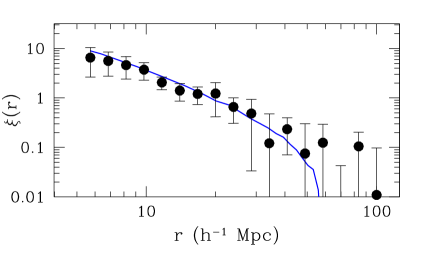
Figure 5: Comaprison of the underline $\Lambda$CDM $S_{1}$-like cluster correlation function (continuous line) with the mean of 6 SDSS mock samples.

Furthermore, we address the issue of the observed anisotropies along the line of sight (see Fig. 4) by searching whether mock obervers show similar $S_{1}$-like clustering elongations along either their $\pi$ or $\sigma$ directions. We quantify this anisotropy by the ratio, ${\cal R}$, of the $\xi(\sigma,\pi)$ in the bins $(\pi,\sigma)=(0-20,20-40)\;h^{-1}$ Mpc (hereafter $\xi_{1,2}$) and $(\pi,\sigma)=(20-40,0-20)\;h^{-1}$ Mpc (hereafter $\xi_{2,1}$).

We have selected 114 independent mock SDSS surveys (by spanning the $z$ coordinate axis of the simulation) and we have found that in the majority of the cases ($\sim$ 60%) the value of ${\cal R}$ is larger than unity, indicating a predominance of anisotropies along the $\pi$ direction, while only $\sim$40% of the cases it is less than one, indicating anisotropies along the $\sigma$ direction.

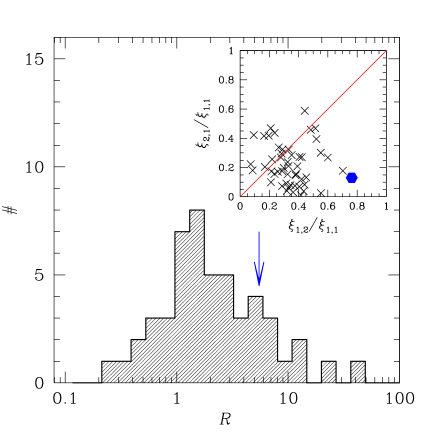
Figure 6: The ${\cal R}=\xi_{1,2}/\xi_{2,1}$ for 50 mock $S_{1}$ like SDSS surveys for which $\xi_{1,2}$ or $\xi_{2,1}$ is larger than 0.4. Note that ${\cal R}>1$ values indicate anisotropies along the $\pi$ direction, while the arrow shows the observed SDSS ${\cal R}$ value. The insert plot shows the amplitude of the anisotropies, with respect to the central value ($\xi_{1,1}$). Note that the continuous line divides anisotropies along the $\pi$ direction (right of the line) and anisotropies along the $\sigma$ direction (left of the line).

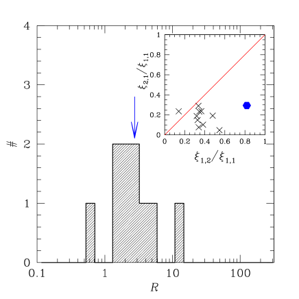
Figure 7: As in Fig.6 but for the $S_{2}$ sample.

We then investigated the amplitude of these $S_{1}$ clustering anisotropies by deriving the distribution of the ${\cal R}$ values for those observers that see relatively high correlation values; $\xi_{1,2}>0.4$ and $\xi_{2,1}>0.4$ (Fig. 6). In total we find 50 such observers out of which 37 (74%) show elongation along their line-of-sight. Therefore, it is evident, also due to the tail towards large ${\cal R}$ values, that there are systematic anisotropies along the line-of-sight, which of course could be only due to the geometric characteristics of the mock cluster distribution. Furthermore in the insert of figure 6 we plot a scatter diagram between the normalized, by the value of $\xi(\sigma,\pi)$ at the first bin (ie., $0<\sigma,\pi<20\;h^{-1}$ Mpc), values of $\xi_{1,2}$ and $\xi_{2,1}$. It is apparent that the observed SDSS value (filled point) is roughly consistent with of the simulation derived values, although it appears to be an extremum. This indicates that the major part of the observed anisotropy is indeed due to the geometrical characteristics of the survey, as we have anticipated in the previous subsection, however we cannot exclude that some small contribution from intrinsic systematics effects, like projection effects (cf. Sutherland 1988), could be present.

A similar analysis of the $S_{2}$ richness cluster correlations has shown that the percentage of mock observers having significant clustering anisotropies along the $\pi$ direction is significantly higher than those seeing anisotropies along the $\sigma$ direction (9 out of 10), however the amplitude of these anisotropies appear to be lower than in the observed case. In Fig. 7 we show the corresponding ${\cal R}$ distribution and the scatter plot, in which it is evident that the amplitude of the true SDSS clustering anisotropy in the $\pi$ direction is quite larger than what expected due to the survey geometrical characteristics.

Therefore, we conclude that in the case of the $S_{1}$ cluster correlations there is no significant evidence for contamination by projection effects, while in the case of the $S_{2}$ correlations we do have such indications. However, in order to perform an a posteriori correction of $\xi(r)$ (cf. Efstathiou 1992), for projection effects it would be necessary to disentangle first the effects of the survey geometry, a task which at the present time is out of the scope of this work. Therefore, we caution the reader that all results based on the $S_{2}$ cluster sample could be affected by the above mentioned systematic effect.

3 Model cluster correlations

It is well known (cf. Kaiser 1984; Benson et al. 2000) that assuming linear biasing the mass-tracer and dark-matter correlations, at some redshift $z$, are related by:

$$\xi_{\rm model}(r,z)=\xi_{\rm DM}(r,z)b^{2}(z)\;\;,$$ (2)

where $b(z)$ is the bias redshift evolution function. In the present work we have used the so called test particle bias model described by Nusser & Davis (1994), Fry (1996) and Tegmark & Peebles (1998). In this case the evolution of the correlation bias is developed assuming that only the test particle fluctuation field is related proportionally to that of the underling mass. Therefore, the bias factor as a function of redshift is

$$b(z)=1+\frac{(b_{\circ}-1)}{D(z)}\;\;,$$ (3)

with $b_{\circ}$ being the bias at the present time and $D(z)$ the linear growth rate of clustering (described in section 4). It has been found (Bagla 1998) that, in the interval $0\leq z\leq 1$, the above formula represents well the evolution of bias. Furthermore, the more accurate linear bias evolution model given by Basilakos & Plionis (2001; 2003) is also very similar to the model of eq.(3) within $z\leq 1$.

We quantify the evolution of clustering with epoch presenting the spatial correlation function of the mass $\xi_{\rm DM}(r,z)$ as the Fourier transform of the spatial power spectrum $P(k)$:

$$\xi_{\rm DM}(r,z)=D^{2}(z)\frac{1}{2\pi^{2}}\int_{0}^{\infty}k^{2}P(k)\frac{{\rm sin}(kr)}{kr}{\rm d}k\;\;,$$ (4)

where $k$ is the comoving wavenumber.

As for the power spectrum, we consider that of CDM models, where $P(k)\approx k^{n}T^{2}(k)$ with scale-invariant ($n=1$) primeval inflationary fluctuations. We utilize the transfer function parameterization as in Bardeen et al. (1986), with the approximate corrections given by Sugiyama’s (1995) formula:

$$T(k)=\frac{{\rm ln}(1+2.34q)}{2.34q}[1+3.89q+(16.1q)^{2}+$$

$$(5.46q)^{3}+(6.71q)^{4}]^{-1/4}\;\;.$$

with

$$q=\frac{k}{\Omega_{\circ}h^{2}{\rm exp}[-\Omega_{b}-(2h)^{1/2}\Omega_{b}/\Omega_{\circ}]}$$ (5)

where $k=2\pi/\lambda$ is the wavenumber in units of $h$ Mpc^-1 and $\Omega_{b}$ is the baryon density.

In the present analysis we consider flat models with cosmological parameters that fit the majority of observations, ie., $\Omega_{\rm m}+\Omega_{Q}=1$, $H_{\circ}=100h$km s^-1 Mpc^-1 with $h\simeq 0.7$ (cf. Freedman et al. 2001; Plionis 2002; Peebles and Ratra 2002 and references therein), baryonic density parameter $\Omega_{\rm b}h^{2}\simeq 0.02$ (e.g. Olive, Steigman & Walker 2000; Kirkman et al 2003) and a CDM shape parameter $\Gamma=0.17$. In particular, we investigate 3 spatially flat low-$\Omega_{\rm m}=0.3$ cosmological models with negative pressure and values of $w=-1$ ($\Lambda$CDM), $w=-2/3$ (QCDM1) and $w=-1/3$ (QCDM2). Note that all the cosmological models are normalized to have fluctuation amplitude, in a sphere of 8 $h^{-1}$Mpc radius, of $\sigma_{8}=0.50(\pm 0.1)\Omega_{\rm m}^{-\gamma}$ (Wang & Steinhardt 1998) with $\gamma=0.21-0.22w+0.33\Omega_{\rm m}$.

4 The linear growth rate of clustering

For homogeneous and isotropic flat cosmologies, driven by non relativistic matter and an exotic fluid (quintessence models) with equation of state, $p_{Q}=w\rho_{Q}$ and $-1\leq w<0$, the Friedmann field equations can be written as:

$$H^{2}=\left(\frac{\dot{\alpha}}{\alpha}\right)^{2}=\frac{8\pi G}{3}(\rho_{\rm m}+\rho_{Q})$$ (6)

and

$$\frac{\ddot{\alpha}}{\alpha}=-4\pi G[(w+\frac{1}{3})\rho_{Q}+\frac{1}{3}\rho_{\rm m}]\;\;,$$ (7)

where $\alpha(t)$ is the scale factor, $\rho_{\rm m}\propto\alpha(t)^{-3}$ is the matter density and $\rho_{Q}\propto\alpha(t)^{-3(1+w)}$ is the dark energy density.

The time evolution equation for the mass density contrast, modeled as a pressureless fluid has general solution of the growing mode (Peebles 1993):

$$\ddot{D}+2H(t)\dot{D}=4\pi G\rho_{\rm m}D\;\;,$$ (8)

where dots denote derivatives with respect to time. From the equations describing the Friedmann model, it follows that $\dot{H}+H^{2}=-4\pi G[(w+1/3)\rho_{Q}+(1/3)\rho_{\rm m}]$. Differentiating this relation and using $\dot{\rho_{\rm m}}=-3H\rho_{\rm m}$ $\dot{\rho_{Q}}=-3(1+w)H\rho_{Q}$ we obtain

$$\ddot{H}+2H\dot{H}=4\pi G(1+w)(w+\frac{1}{3})\rho_{Q}H+4\pi G\rho_{\rm m}H\;.$$ (9)

Therefore, it turns out that if $w=-1$ ($\Lambda$CDM) or $w=-1/3$ (QCDM2) then $H(t)$ is a decaying mode of eq.(8). In that case, the growing solution (Peebles 1993) as a function of redshift is:

$$D(z)=\frac{5\Omega_{\rm m}E(z)}{2}\int^{\infty}_{z}\frac{(1+x)}{E^{3}(x)}{\rm d}x\;\;.$$ (10)

where we have used the following expressions:

$$E(z)=\left[\Omega_{\rm m}(1+z)^{3}+\Omega_{Q}(1+z)^{3(1+w)}\right]^{1/2}$$ (11)

$$\frac{dt}{dz}=-\frac{1}{H_{\circ}E(z)(1+z)}\;\;.$$ (12)

The Hubble parameter is given by: $H(z)=H_{\circ}E(z)$, while $\Omega_{\rm m}=8\pi G\rho_{o}/3H_{o}^{2}$ (density parameter), $\Omega_{Q}=8\pi G\rho_{Q}/3H_{o}^{2}$ (dark energy parameter) at the present time, which satisfy $\Omega_{\rm m}+\Omega_{Q}=1$ and finally $H_{\circ}$ is the Hubble constant. In addition to $\Omega_{m}(z)$ also $\Omega_{Q}(z)$ could evolve with redshift as

$$\Omega_{\rm m}(z)=\frac{\Omega_{\rm m}(1+z)^{3}}{E^{2}(z)}$$ (13)

and

$$\Omega_{Q}(z)=\frac{\Omega_{Q}(1+z)^{3(1+w)}}{E^{2}(z)}\;\;.$$ (14)

It is interesting to mention that in a flat low-$\Omega_{\rm m}$ with $w=-1/3$ model, the equation of state $p_{Q}=-(1/3)\rho_{Q}$ leads to the same growing mode as in an open universe, despite the fact that this quintessence model has a spatially flat geometry! Therefore, as the time evolves with redshift, utilizing equations (12), (11) and the relation

$$4\pi G\rho_{\rm m}=\frac{3H_{\circ}^{2}}{2}\Omega_{\rm m}(1+z)^{3}\;,$$ (15)

then the basic differential equation for the evolution of the linear growing mode takes the following form:

$$\frac{{\rm d}^{2}D}{{\rm d}z^{2}}+P(z)\frac{{\rm d}D}{{\rm d}z}+Q(z)D=0\;\;$$ (16)

with basic factors,

$$P(z)=-\frac{1}{1+z}+\frac{1}{E(z)}\frac{{\rm d}E(z)}{{\rm d}z}$$ (17)

and

$$Q(z)=\frac{3\Omega_{\rm m}(1+z)}{2E^{2}(z)}\;\;.$$ (18)

We find that eq.(16) has a decaying solution of the form $D_{1}(z)=(1+z)^{n}$ only for $w=-2/3$, with $n=3/2$. The second independent solution of eq.(16) can be found easily from the following expression:

$$D(z)=D_{1}(z)\int_{z}^{\infty}\frac{{\rm d}x}{D_{1}^{2}(x)}\;{\rm exp}\left[-\int^{x}P(t){\rm d}t\right]$$ (19)

which finally leads to the following growing mode:

$$D(z)=(1+z)^{3/2}\int_{z}^{\infty}\frac{{\rm d}x}{(1+x)^{2}E(x)}\;\;.$$ (20)

Figure 8: The variance $\Delta\chi^{2}$ around the best fit $b_{\circ}$ value for various cosmological models. The left and the right panel correspond to the $\rm S_{2}$ and $\rm S_{1}$ samples, respectively.

Table 2: List of the theoretical clustering model fitting analysis. Note that the errors of the fitted parameters represent $2\sigma$ uncertainties.

Index	$b_{\circ}$	$\beta$	$K(\beta)$
$\Lambda$CDM-$\rm S_{1}$	$2.4^{+0.2}_{-0.3}$	$0.20^{+0.029}_{-0.016}$	$1.14^{+0.02}_{-0.01}$
QCDM1-$\rm S_{1}$	$2.6^{+0.3}_{-0.2}$	$0.19^{+0.016}_{-0.020}$	$1.13^{+0.01}_{-0.01}$
QCDM2-$\rm S_{1}$	$2.7^{+0.2}_{-0.3}$	$0.18^{+0.023}_{-0.013}$	$1.12^{+0.02}_{-0.01}$
$\Lambda$CDM-$\rm S_{2}$	$1.4^{+0.1}_{-0.1}$	$0.35^{+0.027}_{-0.023}$	$1.26^{+0.02}_{-0.02}$
QCDM1-$\rm S_{2}$	$1.7^{+0.1}_{-0.1}$	$0.29^{+0.019}_{-0.019}$	$1.21^{+0.01}_{-0.01}$
QCDM2-$\rm S_{2}$	$1.7^{+0.1}_{-0.1}$	$0.30^{+0.019}_{-0.016}$	$1.22^{+0.01}_{-0.01}$

5 The SDSS cluster biasing

In order to quantify the cluster bias at the present time we perform a standard $\chi^{2}$ minimization procedure (described before) between the measured correlation function of the SDSS galaxy clusters with those expected in our spatially flat cosmological models

$$\chi^{2}(b_{\circ})=\sum_{i=1}^{n}\left[\frac{\xi_{\rm S_{j}}^{i}(r)-\xi_{\rm model}^{i}(r,b_{\circ})}{\sigma^{i}}\right]^{2}\;\;,$$ (21)

where $\sigma^{i}$ is the observed correlation function (bootstrap) uncertainty.

In Fig. 5 we present, for various cosmological models, the variation of $\Delta\chi^{2}=\chi^{2}(b_{\circ})-\chi^{2}_{\rm min}(b_{\circ})$ around the best $b_{\circ}$ fit, for the different richness class (left panel for $\rm S_{2}$ and right panel for $\rm S_{1}$).

Figure 9: Comparison of the observed and model SDSS cluster correlation function: Left panel, $\rm S_{2}$ sample; right panel, $\rm S_{1}$ sample. The observational data are represented by filled symbols.

To this end, owing to the fact that the observational data are analyzed in redshift space, the correlations should be amplified by the factor $K(\beta)=1+2\beta/3+\beta^{2}/5$ (Hamilton 1992) where $\beta\simeq\Omega_{\rm m}^{\cal{\alpha}}/b_{\circ}$. We utilize the generic expression for ${\cal\alpha}$, defined by the Wang & Steinhardt (1998):

$${\cal\alpha}\simeq\frac{3}{5-w/(1-w)}+\frac{3}{125}\frac{(1-w)(1-3w/2)}{(1-6w/5)^{3}}(1-\Omega_{\rm m})\;\;.$$ (22)

In Table 2 we list the results of the fits for our two cluster catalogs, ie., the cosmological models and the value of the cluster optical bias, $b_{\circ}$, at the present time, as well as the redshift distortion $\beta$ parameter and a measure of the $K(\beta)$ correction. We find that the redshift space distortions effect increases $\xi_{\rm S_{j}}(r)$ by a factor of $\sim 12-26\%$.

In Fig. 6, we plot the measured $\xi_{\rm S_{j}}(r)$ (filled symbols) of our two samples with the estimated two point correlation function for all three cosmological models. We should conclude that the behavior of the observed two point correlation function of the galaxy clusters is sensitive to the different cosmologies with a strong dependence on the present time bias. By separating between low and high richness regimes, we obtain results being consistent with the hierarchical clustering scenario, in which the rich clusters are more biased tracers of the underlying matter distribution with respect to the low richness clusters.

We can put some further cosmological constraints, comparing our clustering results with those based on large-scale dynamics. For example Branchini & Plionis (1996) using the cluster dipole after reconstructing the spatial distribution of Abell/ACO $R\geq 0$ clusters found $\beta_{\rm Abell}=0.21\pm 0.03$. Also, Branchini at al. (2000) comparing the density and velocity fields of the Abell/ACO cluster distribution with the corresponding POTENT fields (using the MARK III galaxy velocity sample), obtained $\beta_{\rm POTENT}=0.22\pm 0.08$. Comparing the latter $\beta$-results with our clustering predictions (Table 2) we can conclude that for the $\rm S_{1}$ sample (Abell $R\geq 0$ richness) the only model which fails (although marginally) to reproduce the large-scale dynamical results is QCDM2 ($w=-1/3$).

6 Conclusions

We have studied the clustering properties of the SDSS galaxy clusters in redshift space. We have divided the total sample in two richness subsamples; roughly corresponding to Abell $R\geq 0$ ($N_{\rm gal}\geq 30$ members) and to APM ($N_{\rm gal}\geq 20$ members) clusters. We find that if the two point cluster correlation function is modeled as a power law, $\xi(r)=(r_{\circ}/r)^{\gamma}$, then the best-fitting parameters are (a) $r_{\circ}=20.7^{+4.0}_{-3.8}\;h^{-1}$ Mpc with $\gamma=1.6^{+0.4}_{-0.4}$ and (b) $r_{\circ}=9.7^{+1.2}_{-1.2}\;h^{-1}$ Mpc with $\gamma=2.0^{+0.7}_{-0.5}$ respectively. We have also found that the Abell-like sample is not significantly affected by projection effects, and its apparent clustering elongation along the line-of-sight is due to the survey geometry. However, the APM-like sample appears to be somewhat affected by projection effects, showing a clustering elongation along the line-of-sight larger than what expected from the survey geometry.

Comparing the cluster correlation function with the predictions of 3 spatially flat quintessence models (having $\Omega_{\rm m}=0.3$), we estimate the cluster redshift space distortion parameter $K(\beta)$ and we conclude that the amplitude of the cluster redshift correlation function increases by a factor of $\sim 12-26\%$ (depending on the richness class). Finally, comparing our clustering results with those of dynamical analysis, based on the large scale motions, we find that the flat cosmological models with $w\leq-0.6$ are consistent with the observational results.

References

- [] Abadi, M. G., Lambas, D. G., Muriel, H., 1998, ApJ, 507, 526
- [] Bardeen, J.M., Bond, J.R., Kaiser, N. & Szalay, A.S., 1986, ApJ, 304, 15
- [] Bagla J. S. 1998, MNRAS, 417, 424
- [] Bahcall, N., &, Soneira, R. M., 1983, ApJ, 270, 20
- [] Bahcall, N., &, Burgett, W. S., 1986, ApJ, 300, L35
- [] Bahcall, N., &, West, M. J., 1992, ApJ, 392, 419
- [] Basilakos, S. & Plionis, M., 2001, ApJ, 550, 522
- [] Basilakos, S. & Plionis, M., 2003, ApJ, 593, L61
- [] Benson A. J., Cole S., Frenk S. C., Baugh M. C., & Lacey G. C., 2000, MNRAS, 311, 793
- [] Borgani, S., Plionis, M., Kolokotronis, V., 1999, MNRAS, 305, 866
- [] Branchini, E., &, Plionis. M., 1996, ApJ, 460, 569
- [] Branchini, E., Zehavi, I., Plionis. M., & Dekel, A., 2000, MNRAS, 313, 491
- [] Colberg, J.M., et al., 2000, MNRAS, 319 209
- [] Collins, C. A., et al., 2000, MNRAS, 319, 939
- [] Croft, R., A., C., Dalton, B., Efstathiou, G., Sutherland, W., J., Maddox, S., J., 1997, MNRAS, 291, 305
- [] Dalton, B. G., Croft, R. A. C., Efstathiou, G., Sutherland, W. J., Maddox, S. J., Davis, M., 1994, MNRAS, 271, L47
- [] Efstathiou, G., Dalton, B. G., Sutherland, W. J., Maddox, S. J., 1992, MNRAS, 257, 125
- [] Freedman, W., L., et al., 2001, ApJ, 553, 47
- [] Frenk, C.S., et al, 2000, astro-ph:0007362
- [] Fry J.N., 1996, ApJ, 461, 65
- [] Fukugita, M., Shimasaku, K., Ichikawa, T. 1995, PASP, 107, 945
- [] Gonzalez, A. H., Zaritsky, D., Wechsler, R. H., 2002, ApJ, 571, 129
- [] Goto, T., et al., 2002, AJ, 123, 1825
- [] Hamilton, A. J. S., 1992, ApJ, 385, L5
- [] Hamilton, A. J. S., 1993, ApJ, 417, 19
- [] Jing, Y.P., Plionis, M., Valdarnini, R., 1992, ApJ, 389, 499
- [] Kaiser N., 1984, ApJ, 284, L9
- [] Kirkman, D., Tytler, D., Suzuki, N., O’Meara, J.M., Lubin, D., 2003, ApJS submitted, astro-ph/0302006
- [] Klypin, A. A. & Kopylov, A. I., 1983, Sov.Astr.Let., 9, 41
- [] Lahav O., Edge, A. C., Fabian, A. C., Putney, A., 1989, MNRAS, 238, 881
- [] Mo, H. J., Jing, Y. P., Brner, G., 1992, ApJ, 392, 452
- [] Moscardini, L., Matarrese, S., Mo, H. J., 2001, MNRAS, 327, 422
- [] Nichol, R. C., Briel, O. G., Henry, P. J., 1994, ApJ, 267, 771
- [] Nusser & Davis, 1994, ApJ, 421, L1
- [] Olive, K.A., Steigman, G., Walker, T.P., Phys.Rep., 333, 389
- [] Peacock, A. J., &, West, M., 1992, MNRAS, 259, 494
- [] Peacock, A. J., &, Dodds, S. J., 1994, MNRAS, 267, 1020
- [] Peebles P.J.E., 1993. Principles of Physical Cosmology, Princeton University Press, Princeton New Jersey
- [] Peebles P.J.E., Ratra, B., 2003, astro-ph/0207347
- [] Plionis, M., &, Basilakos, S., 2002, MNRAS, 329, L47
- [] Plionis, M., in Cosmological Crossroads, Springer LNP, 592, p.147 (eds. Cotsakis & Papandonopoulos)
- [] Sugiyama, N., 1995, ApJS, 100, 281
- [] Tago, E., Saar, E., Einasto, J., Einasto, M., Müller, V., Andernach, H., AJ, 123, 37
- [] Tegmark M. & Peebles P.J.E, 1998, ApJL, 500, L79
- [] Wang, L. & Steinhardt, P.J., 1998, ApJ, 508, 483