THE SPATIAL DISTRIBUTION OF FLUORESCENT H₂ EMISSION NEAR T TAU

Abstract

New subarcsecond FUV observations of T Tau with HST/STIS show spatially resolved structures in the 2”$\times$2” area around the star. The structures show in multiline emission of fluorescent H₂ pumped by Lyman $\alpha$. One emission structure follows the cavity walls observed around T Tau N in scattered light in the optical. A temperature of $\geq$ 1000K is required to have enough population in the H₂ to produce the observed fluorescent lines; in the cool environment of the T Tau system, shock heating is required to achieve this temperature at distances of a few tens of AU. Fluorescent H₂ along the cavity wall represents the best evidence to date for the action of low-density, wide-opening-angle outflows driving cavities into the molecular medium at scales $\leq 100$ AU. A southern region of emission consists of two arcs, with shape and orientation similar to the arcs of H₂ 2.12 $\mu m$ and forbidden line emission crossing the outflow associated with the embedded system T Tau S. This region is located near the centroid of forbidden line emission at the blueshifted lobe of the N-S outflow.

1 Introduction

T Tau is a multiple system of pre-main sequence stars, composed of an optically-visible K0 star, T Tau N, and a heavily-extincted system, T Tau S (Dyck et al., 1982), which is itself binary (Koresko, 2000; Köhler et al., 2000; Duchêne et al., 2002). The T Tau system is surrounded by an infalling envelope of a few thousand AU (Calvet et al., 1994), which is in the process of being disrupted by powerful outflows (Momose et al., 1996). Two bipolar outflows have been identified in the system (Solf, Böhm, & Raga, 1988; Böhm & Solf, 1994). One of the outflows runs NW-SE and has been associated with the embedded pair T Tau S. Analysis of the forbidden line emission indicates that this outflow is poorly collimated (Böhm & Solf, 1994; Solf & Böhm, 1999). Bright arcs of forbidden line emission (Robberto et al., 1995) and near infrared H₂ line emission (Herbst et al., 1996, 1997) are found crossing this outflow at scales of $\sim$ 2” - 14” ($\sim$ 280 - 2000 AU at the distance of Taurus, 140 pc, Kenyon et al. 1994). Burnham nebula, $\sim$ 8” south of the system, is associated with the blueshifted lobe of this outflow; it continues in jets detected out to $\sim$ 0.7 pc (Reipurth et al., 1997). The other outflow runs E-W and is associated with T Tau N. It is less bright in the optical, although high velocity forbidden line emission is detected towards the west, ending in Herbig Haro object HH155 located at the edge of the reflection nebulosity NGC 1555 (Hind’s nebula), $\sim$ 35” west from the star. ¹²CO emission associated with the E-W outflow shows blue and redshifted lobes of moderately high velocity (Schuster et al. 1994), surrounded by rings of ¹³CO emission at lower velocity; these rings have been interpreted as arising at the wall of the cavity in the envelope opened by the E-W outflow (Momose et al. 1996).

The structure of the outflows and molecular gas and dust very near T Tau (inner 2”x2”) is uncertain. Observations in the V, R, and I filters with the WFPC2 camera on the Hubble Space Telescope ($HST$) by Stapelfeldt (1998, S98) showed a scattered light structure whose morphology suggests an illuminated outflow cavity in the circumsystem envelope. Spectroscopic mapping in the K (2.01-2.42 $\mu$m) and H (1.5-1.8 $\mu$m) bands by Kasper et al. (2001) probed the inner 2”$\times$2” of the T Tau system; unresolved Br$\gamma$ emission at the positions of T Tau N and S was observed, but no infrared H₂ emission was detected.

In contrast, space-based observations in the UV of molecular hydrogen have indicated structure on small scales near T Tau. Brown et al. (1981) detected extended H₂ fluorescent emission in T Tau N and its adjacent nebula in a low resolution large aperture spectrum from the IUE satellite. Valenti et al. (2000) refined the location of the H₂ emission by comparing data from the Goddard High Resolution Spectrograph (GHRS) on $HST$ in G140L mode with all the available IUE spectra of T Tau. The H₂ line fluxes were found to be larger in the IUE spectra suggesting that the molecular hydrogen emission extended beyond 0.2” from the star, the size of the Small Science Aperture in GHRS. In this paper, we present new data from the Space Telescope Imaging Spectrograph (STIS) on board $HST$ which illustrate the spatial distribution of fluorescent H₂ emission in the T Tau system, with important implications for the interaction of outflows and circumstellar matter.

2 Observations

T Tauri was observed with $HST$ on 2000 February 7 in program GO8317, using the STIS MAMA detector with the G140L grating. A 2” long slit with a PA=$30^{\circ}$ was employed, and the data were taken in binned pixels mode with an exposure time of 1622 s. The spectral range covered from 1118 to 1715 Å with a dispersion of 0.58 Å per pixel resulting in a resolution of $\sim$1 Å at 1500 Å, and a plate scale of 0.024” per pixel. Standard CALSTIS pipeline procedures were used to reduce the data.

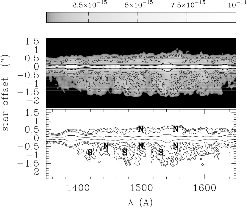
Figure 1: Position-dispersion image of T Tau N between 1350 and 1650 Å. The upper panel shows the observed spectrum. The isocontours have values of 0.65e-15, 0.8e-15 1.0e-15 and 3.0e-15 erg cm^-2 s^-1 Å^-1 pix^-1. The extended emission is evident, specially at negative offsets from the star. The lower panel shows the same isocontours, identifying some the features described in the text. Note the groups of periodic features, one close to the stellar spectrum, marked N, and another to the south, marked S, displaced redwards respect to the first. The location of the extraction boxes used to obtain the envelope spectra in indicated in the upper panel.

Figure 1 shows the position-dispersion image. Faint emission is seen extending roughly 1.6” $\sim$ 240 AU southward from the ultraviolet image of T Tau N. Some extended emission is seen to the north, but to a much smaller extent. The spectra of the extended emission were extracted using standard IRAF/STSDAS/X1D tasks, although the extraction was difficult because the spectra have low signal-to-noise ($\sim$ 8 for the strongest lines) and because extended structures fill the large aperture in the dispersion direction. For the extraction, the position of the background was taken outside of the range corresponding to the geocoronal Lyman $\alpha$ and O I lines and far from the extended emission; the background was the same for all the spectra, averaged over 10 pixels. The signal along the extended emission is weak, roughly 20 times weaker than the stellar spectrum. Line emission accounts for about 50% of the total signal. We attempt to identify the strongest emission features, recognizing that there may be weaker, more diffuse emission that we cannot trace.

Figure 2 shows the spectrum of T Tau N, scaled by a factor of 0.2, and spectra extracted in 10 pixel = 0.24” boxes at various offsets from the star along the slit orientation. Lines from the highly-ionized species Si IV 1393/1402, C IV 1458/1550, and He II 1640 are present in the stellar spectrum; the corresponding emission features in the spectra offset at $\pm$ 0.39” are consistent with the expected wings of the instrumental point spread function for the stellar emission. The other line features in the extended nebulosity are consistent with fluorescent H₂ emission. As shown in Figure 2, the strongest lines arising from de-excitation of the rotational-vibrational level (v’,J’=1,4) of the electronic state ${}^{1}\Sigma_{u}^{+}$ populated by the (1-2)P(5) transition can be identified. There is also a suggestion that the strongest lines of the de-excitation of the (v’,J’=1,7) level, populated by the (1-2)R(6) transition are present.

Table 1 shows the observed fluxes of the fluorescent lines due to the (1-2)P(5) transition in several offset spectra. The fluxes are measured above the estimated continuum. The last column shows the ratios of the line fluxes at $\lambda 1446$ and $\lambda 1504$ Å, where the fluxes have been corrected for reddening with A_V=2.2 using the HD29647 extinction law (Calvet et al., 2003). The ratios are consistent with the optically thin ratio (0.73), within the uncertainties given by their low S/N.

3 Spatial distribution

To make the line identifications shown in Figure 2, it is necessary to impose wavelength shifts to the spectra of the extended emission. If these shifts were interpreted as velocities, they would require motions of $\sim$ 2000 km s^-1 or more, much larger than the velocities previously reported in the region ($\sim$ 45 km s^-1; (Böhm & Solf, 1994; Eislöffel & Mundt, 1998). A more likely explanation for the wavelength shifts is that they are due to spatial shifts of the emission regions relative to the star within the large (2”) aperture. In this case, the wavelength shift $\Delta\lambda$ would imply a displacement $x=s\Delta\lambda/m$ from the axis of the slit, where $s$ is the plate scale and $m$ is the dispersion. All the offsets are measured from the position of T Tau N.

Figure 2 indicates at the right the offsets $x$ required to fit the H₂ lines at each $y$ offset from the star. Two spatially-distinct regions of H₂ emission can be identified. One region extending to $y\sim 0.7$” southwest from the star, which is shifted slightly westwards, and a region covering $0.7"<y<1.6"$ from the star, which has an eastward displacement. These regions can be discerned in Figure 1. The northern region, labeled by N in the sketch below the spectrum in Figure 1, can be seen as three features extending to a distance of about 0.7” southward from the star, at PA $\sim 210^{\circ}$, corresponding to the H₂ line pairs at 1490/1505 Å, 1431/1446 Å, and 1547/1562 Å, although in the latter case the structure near the star is difficult to see due to the strong stellar C IV 1550 Å emission. Further south, these emission features seem to disappear; however, similar pairs of emission lines can be seen shifted roughly 25 Å blueward, extending nearly vertically in the image to about 1.6” south. This region of emission is labeled S in Figure 1. The N region extends to the north of the star as well, but it is difficult to identify spectral features in it. After taking into account the position angle of the slit, we find that the spatial location of the upper N emission region appears to correspond to the the brightest part of the southern optical scattered light structure imaged by S98, while the lower emission region roughly follows the outer border of the scattered light nebula, although displaced from it.

To obtain more information about the spatial distribution of the emission, we constructed a model and compare the predicted emission with the observed spectrum. If the spatial distribution of the emission at a given offset $y$ is given by w(x,y), and the intrinsic emission at each point is $G_{\lambda}$, then the observed flux at wavelength $\lambda$ is given by the convolution of w(x,y) and $G_{\lambda}$,

$${\it F}_{\lambda}(y)=a\sum_{i=1}^{N}G_{\lambda-\Delta\lambda_{i}}w(x(i),y)$$ (1)

where $a$ is a scaling constant, x(i) is the spatial shift across the slit from its axis, $\Delta\lambda_{i}$ is the wavelength shift corresponding to $x(i)$, and $N$ is the number of pixels across the slit.

We used as template $G_{\lambda}$ the spectrum of HH 43, a low-excitation Herbig-Haro object, which clearly shows the fluorescent lines we have identified (Schwartz, 1983). The spectrum is an average of the three IUE large aperture spectra with the highest exposure times, SWP31828, SWP23881, and SWP24924, taken from the Multimission Archive at the Space Telescope Science Institute, which have been processed under the NEWSIPS extraction pipeline. The combined signal to noise of the resultant HH spectrum is 8-13. Since we are interested in the relative distribution of the H₂ intensity, we normalized $w(x,y)$ to 1 and scaled $G_{\lambda}$ with the constant a to fit the observed spectrum of the extended emission at offset $y$ = -0.39”.

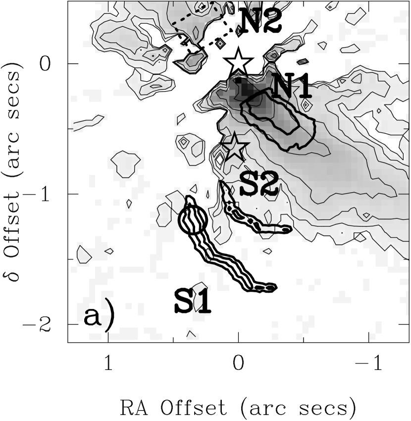
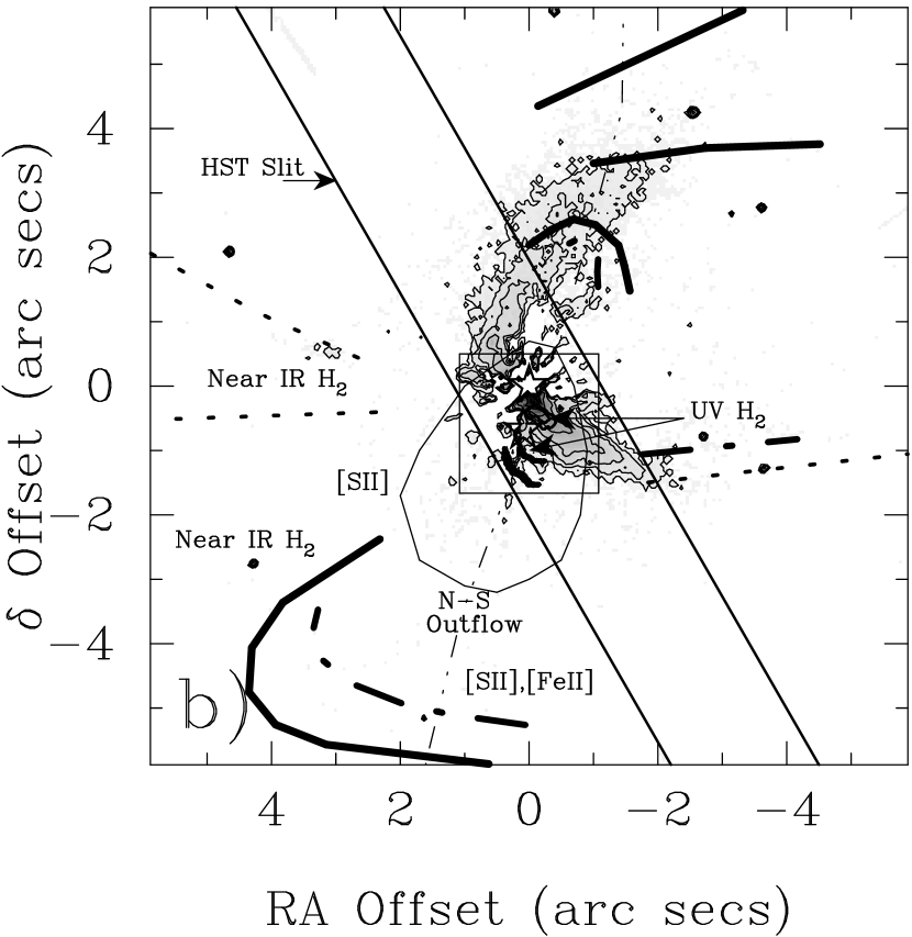
Figure 4: Spatial distribution of the H₂ emission. a): Isocontours of fluorescent H₂ emission (thick solid lines) superimposed on magnitude isocontours of 0.55 $\mu$m emission from Stapelfeldt et al. (1998) (relative intensity grayscale/thin lines). The isocontours for the fluorescent features show relative intensity, with steps of 1 magnitude, corresponding to values of 1, 0.398 and 0.158. The regions discussed in the text, N1, N2, S1, and S2 are indicated. The mean centroid position of component D from Böhm & Solf (1994) is also shown (open circle). The dotted box shows an estimate for the location of region N2, since the overextraction of the star in the optical image makes it difficult to obtain a brightness distribution (S98). b): View of a larger area around the region shown in the upper panel (indicated by the box), showing the observing slit and features discussed in the literature: Terminal H₂ shocks (thick lines), [S II] or [Fe II] shocks (dot-dashed line), oblique H₂ shocks (dashed lines), from Herbst et al. (1997), associated to the N-S outflow. The extend of of component D from Böhm & Solf (1994) is also shown (lobe shaped contour).

The predicted spectra at several offsets $y$ from the star are shown in Figure 3 compared to the observed spectra smoothed to the IUE resolution of 6 Å; the corresponding spatial map of the emission $w(x,y)$ is shown in Figure 4.

The H₂ emission in the southern part of region N (N1 in Figure 4) appears to follow the brightness and spatial distribution of the scattered light image of S98, with some indication that the H₂ is somehow spatially more concentrated than the optical region. The H₂ and optical emission are similar from $\sim$ 0.”45 to $\sim$ 0.”65 from the star, but around $\sim$ 0.”45, the H₂ emission is $\sim$ 30% narrower than the optical scattered light. Consistently, the H₂ emission in the northern part of region N (N2 in Figure 4) is low, since the north part of the optical emission is two magnitudes fainter than the southern portion at the same distance from T Tau N (S98).

The resulting predicted spectra for region N1 are shown at -0.39” and -0.62” offsets in Figure 3. The spectral agreement is reasonable considering the low S/N of the spectra and the contamination by stellar emission at -0.39”. The principal failing of the model is the lack of predicted emission near 1600-1620 Å, which is identified in the spectrum of T Tau N as a mix of CII an Fe II by Valenti et al. (2000). Fe II emission may arise from the $\sim$40 $\rm km~{}s^{-1}$ J-shocks discussed below as sources of Lyman $\alpha$ photons for the lower emission region. It is also likely that the broad Lyman $\alpha$ emission profile of T Tau produces some of the fluorescent sequences observed in Mira (Wood, Karovska, & Raymond, 2002) but not in low excitation HH objects. Some of these sequences include emission near 1610 Å.

For region S, $y\leq-0.85"$, the observed line profiles are too narrow to resolve the emitting regions; we found the best fits by introducing two narrow structures at slightly different positions, labeled S1 and S2 in Figure 4. The agreement between predicted and observed spectra in Figure 3 is reasonably satisfactory except for a feature near 1600-1620 Å in the $y=-0.62"$ offset spectrum. We should also emphasize again that it would be difficult for us to detect very spatially-extended H₂ emission in our large aperture data.

4 Physical conditions

4.1 Estimates of Lyman $\alpha$ luminosities

The total observed flux in the strongest H₂ line we observe, (1-7)P(5), $\lambda$= 1504.8 Å, can be written as (cf. Jordan et al. 1978)

$$F_{H_{2}}=3\times 10^{-16}\,N(2,5)A_{H_{2}}\,\bar{J}_{\nu}\,{\rm\;erg\;cm^{-2}\;s^{-1}},$$ (2)

where $N$(2,5) is the column density in the vibrational-rotational level (v”,J”=2,5) of H₂, $A_{H_{2}}$ is the H₂ emitting area projected in the sky in arcsec², and $\bar{J}_{\nu}$ is the mean intensity of the Lyman $\alpha$ radiation capable of exciting the (1-2)P(5) transition, in ${\rm\;erg\;cm^{-2}\;s^{-1}\;Hz^{-1}}$. We have used the line parameters $B_{(2,5\to 1,4)}=1.976\times 10^{8}$ erg^-1 cm² s^-1, $A_{(1,4\to 7,5)}=1.969\times 10^{8}$ s^-1 and $\Sigma_{j}A_{(1,4\to j)}=1.7125\times 10^{9}$ s^-1 from Abgrall et al. (2000).

If we assume that the H₂ emission region N is irradiated by stellar Lyman $\alpha$ and that there is no extinction between the star and the region, then the mean intensity $\bar{J}_{\nu}$ reaching the region is related to the specific intensity $\bar{I}_{\nu}$ leaving the star by

$$\bar{J}_{\nu}\approx{1\over 4\pi}{{\bar{I}_{\nu}A_{Ly\alpha}}\over d^{2}},$$ (3)

where $A_{Ly\alpha}$ is the area of the Lyman $\alpha$ emitting region on the star and $d$ the distance between the star and the site where the H₂ molecules are pumped. In turn, $\bar{I}_{\nu}$ can be expressed in terms of the flux $\bar{F}^{obs}_{Ly\alpha}$ of Lyman $\alpha$ observed at Earth, as $\bar{I}_{\nu}=\bar{F}^{obs}_{Ly\alpha}D^{2}/A_{Ly\alpha}$ (assuming isotropic emission) where $D$ is the distance to the star. Combining these expressions, we can write

$$\bar{J}_{\nu}\approx 3.3\,\times 10^{9}{\bar{F}^{obs}_{Ly\alpha}\over\theta^{2}}{\rm erg\;cm^{-2}\;s^{-1}\;Hz^{-1}\;sr^{-1}},$$ (4)

where $d/D$ has been approximated by the apparent angular separation between the star and the H₂ emitting region on the sky, $\theta$, in units of arcsec in eq.(4).

Inserting in eq. (2) we obtain

$$F_{H_{2}}\approx 10^{-6}{A_{H_{2}}\over\theta^{2}}N(2,5)\bar{F}^{obs}_{Ly\alpha}{\rm\;erg\;cm^{-2}\;s^{-1}}$$ (5)

We estimate a lower limit for $N$(2,5) by taking the column density of the outermost layers of the cavity where radiation of Lyman $\alpha$ can penetrate, to a depth where $\tau_{\nu}\sim 1$. The actual column density producing the emission may be larger than this if the emitting region is not seen face-on. This may be indeed the case, given the low inclination to the line of sight, $\sim 10^{\circ}$, of the E-W outflow estimated by Momose et al. (1996). The optical depth for a transition line from an upper level j to a lower level i can be written as $\tau_{\nu}=N_{i}B_{ij}h\nu_{ij}\phi_{\nu}(1-exp(-h\nu_{ij}/kT))/4\pi\sim N_{i}B_{ij}h\nu_{ij}\phi_{\nu}/4\pi$, for a temperature of a few thousand K, with $\nu_{ij}$ the frequency of the transition. We assume that the H₂ line is Gaussian in shape, with a Doppler width $\Delta\nu_{D}=\nu_{ij}\sqrt{v_{th}^{2}+v_{tur}^{2}}/c$. The agreement with the spectrum of HH43 (§3) suggests a low excitation situation, so we adopt a temperature T$\sim$1000 K to determine the thermal velocity $v_{th}$, and assume a turbulent velocity $v_{tur}\sim$10 km s^-1 as expected from an oblique shock interface (§5.1). Assuming the line profile is given by $\phi_{\nu}\approx 1/\pi^{1/2}\Delta\nu_{D}$, we get a column density $N(2,5)\approx 7\times 10^{14}$ cm^-2 from the condition $\tau_{\nu}\sim 1$ for the (1-2)P(5) transition.

Let $Q$ be the ratio between $\bar{F}^{obs}_{Ly\alpha}$ and the total observed flux $F_{Ly\alpha}$. We cannot use the stellar Lyman $\alpha$ line profile in the spectrum because it has been heavily absorbed by circumstellar and interstellar extinction. So, we estimate the value of $Q$ assuming that the Lyman $\alpha$ profile is similar to that of Mg II 2800 Å, since both are resonant lines with extended wings formed by partial redistribution. We use the high resolution line profile of Mg II k $\lambda$ 2796.3 in T Tau N, obtained with STIS/NUV-MAMA and echelle grating E230M in our $HST$ program GO8627 (Fig. 5, Saucedo et al., in preparation). At $\Delta v$= 98 km s^-1 from the center of the Mg II 2796.3 Å line, we determine $Q\sim 1.4\times 10^{-12}$ Hz^-1. As illustration, we show in Figure 5 the H₂ line profile $\phi_{\nu}$ at $\Delta v$= 98 km s^-1 used for the calculation of $\bar{F}^{obs}_{Ly\alpha}$.

The emitting area $A_{H_{2}}$ can be estimated from the height of the extraction box used to obtain the spectra and the width of the relative intensity map w(x,y) as $\sim$ 0.2$\times$0.24 arcsec². Taking the distance $\theta$ between the star and the H₂ region as $\sim$ 0.5”, an average flux of H₂ 1504.8 Å $\sim 2.5\times 10^{-15}$ ${\rm erg\;cm^{-2}\;s^{-1}}$ in region N (cf. Table 1), the estimated values of $N(2,5)$ and $Q$, and eq. (5), we can write for the luminosity of the stellar Lyman $\alpha$ line

$$8\times 10^{-3}L_{\odot}\leq L_{Ly\alpha}\leq 2.1L_{\odot}$$ (6)

where the limits arise from the uncertainty in the reddening correction appropiate to the H₂ lines, since the extinction along the line of sight of the nebulosity may not be the same as the extinction of the star; the lower limit comes from taking the observed H₂ flux and the upper limit from dereddening this flux by the extinction to T Tau N, $A_{v}=2.2$ (Calvet et al., 2003). In addition, as discussed above, the actual value of $N(2,5)$ is likely to be higher because of projection effects, making the required Lyman $\alpha$ luminosity lower than estimates in eq.(6). These limits for the Lyman $\alpha$ luminosity are consistent with those obtained by scaling by a factor of 30 the dereddened flux of the CIV 1548 line in our stellar spectra, as suggested by Ardila et al. (2002). With F${}_{\rm CIV}\sim 9.2\times 10^{-12}$ $\rm erg\;cm^{-2}\;s^{-1}$, the scaled Lyman $\alpha$ luminosity would be $\sim$ 0.35 L_⊙.

The estimated maximum Lyman $\alpha$ luminosity (eq. [6]) is $\leq$ 60 % of the accretion luminosity of T Tau N estimated from the NUV spectrum obtained simultaneously with the FUV spectrum, ${\rm L_{acc}=3.2L_{\odot}}$ (Calvet et al., 2003), so it can be accounted for by accretion energy. We thus conclude that the H₂ emission in region N is consistent with stellar Lyman $\alpha$ pumping.

While the bright rims seen in region N are clearly illuminated by T Tau N, the southern arcs S1 and S2 appear to be located (in projection) well inside the envelope, roughly tracing the outer edge of the extended emission of S98. Lyman $\alpha$ from the visible star will be absorbed by dust in the envelope so it cannot penetrate more than one dust mean free path, $l\sim 3-4$ AU, estimated from models of infalling envelopes (Whitney & Hartmann, 1993) with typical envelope parameters from Calvet et al. (1994) ($\rm\dot{M}=3\times 10^{-6}\;M_{\odot}\;yr^{-1},\;r_{c}=100\;AU,\;M=2\;M_{\odot}$) and a dust opacity at the Lyman $\alpha$ wavelength of 1538 cm² g^-1 (Osorio et al., 2002). It is therefore more likely that the required Lyman $\alpha$ emission comes from the shocks themselves, as in the case of low excitation HH objects (Curiel et al., 1995).

If Lyman $\alpha$ is locally produced, then $\bar{J}_{\nu}=\bar{I}_{\nu}/2$, so we can write

$$L_{H_{2}}=6.8\times 10^{-6}N(2,5)QL_{Ly\alpha}$$ (7)

where $L_{H_{2}}=4\pi D^{2}F$ is the H₂ luminosity. Using similar values of $N(2,5)$ and $Q$ as in region N, we get that the luminosity in Lyman $\alpha$ required to excite the H₂ fluorescence in region S is

$$3.4\times 10^{-4}L_{\odot}\leq L_{Ly\alpha}\leq 0.1L_{\odot},$$ (8)

where again, the lower limit is given by the observed values of the H₂ flux, and the upper limit by assuming that the extinction is the same as towards T Tau N, although there is no argument to support the assumption of an homogeneous extinction in the whole region. These limits are consistent with values of the Lyman $\alpha$ luminosity in low excitation HH objects; for instance, Curiel et al. (1995) find $L_{Ly\alpha}\sim 0.13L_{\odot}$ in HH 47A.

4.2 Estimates of temperature and Hydrogen column density

Fluorescence requires a significant population in excited levels which also can lead to infrared H₂ emission lines. Thus, the observed upper limits to the infrared emission line fluxes in observations covering region N (Kasper et al., 2001) can provide an additional constraint on molecular column densities.

An upper limit for the 2.12 $\mu$m H₂ line can be estimated from the equivalent width of 0.15 Å, which is the detection threshold for features in the Kasper et al. (2001) observations. Using the continuum flux of $\sim 3.1\times 10^{-9}{\rm erg\;cm^{-2}\;s^{-1}\mu m^{-1}}$, we obtain that the flux at the 2.12 $\mu$m H₂ line needed for a 2 $\sigma$ detection would be $9.3\times 10^{-14}$ $\rm erg\;cm^{-2}\;s^{-1}$.

The flux at 2.12 $\mu$m H₂ in the optically thin limit is given by $F_{2.12}=I_{2.12}A_{H_{2}}/D^{2}=N(1,3)A_{31}h\nu_{31}/4\pi A_{H_{2}}/D^{2}$, where $N(1,3)$ is the column density of the upper level of the transition. With the Einstein value $A_{31}=3.66\times 10^{-7}s^{-1}$ (Gautier et al., 1976) and the upper limit for the flux, we obtain $N(1,3)\leq 2.24\times 10^{18}{\rm\;cm^{-2}}$.

As mentioned before, we have only a lower limit to the actual N(2,5). With this lower limit and the upper limit for N(1,3), we can obtain a lower limit to the excitation temperature in region N through the Boltzmann relation $N(1,3)/N(2,5)=1/1.57exp(-E_{(1,3\to 2,5)}/kT)$, with $E_{(1,3\to 2,5)}/k\approx 6840$ (Herzberg, 1950). Using our estimates, we obtain $T\geq$ 800 K, consistent with a low velocity shock. From Figures 6 and 7 in Jordan et al. (1978), the population of the levels with (v”J”=2,5) in this temperature range is $\sim$ 12% of the populations with v”=2 and any J”, and in turn, the population with v”=2 is $\sim$ 0.001% of the total population. So, with $N(2,5)>$7$\times 10^{14}$ cm^-2, the column density of the H₂ molecule is N(H₂)$>5.8\times 10^{20}$ cm^-2.

We have no measurements of H₂ 2.12 $\mu$m in region S to help constrain the temperature and total H₂ density. Information on regions S1 and S2 can be obtained from the [O I], [N II] and [S II] PV diagrams in Böhm & Solf (1994). From their Figure 5, regions S1 and S2 are located within one of the multiple components identified in their work, component D, which corresponds to the blueshifted lobe of the N-S outflow. The line ratios [O I]/[S II], [N II]/[O I] and [N II]/[S II] around the location of region S are 1.25, 0.35 and 0.28, respectively. Comparison with shock model predictions Hartigan et al. (1987) indicate a shock of velocity v=40 km s^-1. For this shock velocity, the ratio of Lyman $\alpha$/[O I] can be obtained from these models, yielding a value of $\sim$ 73; so, a rough estimate of the [O I] luminosity is $4.6\times 10^{-6}L_{\odot}\leq L_{[OI]}\leq 3.5\times 10^{-4}L_{\odot}$. Unfortunately, measurement of absolute fluxes for [O I] to compare with this prediction are not available (Solf 2002, private communication). Inspection of the relative intensities of [O I] along the slit with PA=0^∘ centered on the star in Böhm & Solf (1994) indicates that the region at $\sim$ 2 arcsec south is $\sim$ 4-5 times fainter than the star. We can estimate the [O I] stellar luminosity from the mass loss rate $\dot{\rm M_{w}}$, using the relationship log $\dot{\rm M_{w}}=-4.3+{\rm log}(L_{[O\;I]}/L_{\odot})$ (Hartigan et al., 1995), assuming that outflow rate scales as $\sim$ 0.1 the accretion rate (Calvet, 1998), and obtaining the mass accretion rate from the accretion luminosity. This finally leads us to an estimate of $\rm L_{[OI]}\sim 2\times 10^{-4}L_{\odot}$ for the region, which is consistent with our expected limits of the [O I] luminosity.

5 Discussion

5.1 The northern H₂ emitting region

Region N appears to be aligned along the bright rims of the reflection nebulosity around T Tau N, §3; which was plausibly interpreted by S98 as the walls of a cavity driven into the surrounding medium by the outflow from this star. The H₂ emission requires some heating to excite molecules into the level which can fluoresce with Lyman $\alpha$. At distances of $\leq 50$ AU where the fluorescent emission is observed, local dust temperatures resulting from heating by the central star(s) are predicted to be $\sim 100$ K (Calvet et al., 1994), whereas excitation temperatures must be $\geq 800$ K by the argument of the previous section. The most likely explanation is that shock heating is responsible for the excitation of H₂ in these regions, as also suggested by the consistency of the observed spectrum with that of a low-excitation Herbig-Haro object (§3).

The impact of the wind emanating from T Tau N on the molecular medium can naturally explain the needed excitation of H₂, and it has already being suggested as a possible explanation for the near infrared H₂ bright rims that seem to coincide with the scattered light image at larger scales (Herbst et al., 1997). Böhm & Solf (1994) argued that the E-W outflow is a highly collimated, high velocity $\sim$ 200 ${\rm kms^{-1}}$ jet at 0.3” $\sim$ 40 AU from the star from analysis of the forbidden line emission. Alternatively, as proposed previously by Shu et al. (1995), Shang et al. (1998), and more recently by Shang et al. (2002), the jet results from a density enhancement along the outflow axis in a wide-angle wind. Our observations support the second hypothesis in that a wide-angle wind is required to produce the excitation along the walls of the cavity. Moreover, we expect that an oblique shock would be formed at the interaction of the wide-angle wind and the molecular environment, as envisoned by Cantó (1980). Only the normal component of the velocity would be thermalized, reducing the effective pre-shock velocity. The velocities required to produce a low excitation spectrum as that emitted along the cavity (§3) are $\leq$ 60 km s^-1 (Hartigan et al., 1987); higher velocities would result in high ionization UV lines, such as CIV and Si IV, which are clearly absent in our data. Thus, the observed H₂ fluorescent emission at the cavity walls may be the clearest (though indirect) evidence to date for the presence of low-density, wide-opening-angle outflows driving cavities into the molecular medium in star-forming regions.

Observations of other shock-excited features close to T Tau N are needed to help constrain wide-angle wind properties.

5.2 The southern H₂ emitting regions

The double arcs of region S are located as close as 0”.3 (49 AU) to T Tau S. The shape and orientation of this double arc are very similar to the arcs of H₂ 2.12 $\mu m$ and optical forbidden line emission described by Herbst et al. (1996, 1997), interpreted as terminal shocks of H₂, [S II] and [Fe II] (Herbst et al., 1997; Robberto et al., 1995) in the N-S outflow. Figure 4b shows an enlarged view of the region around the T Tau system, indicating the positions of regions N and S and the shocked structures described by Herbst et al. (1997), as well as the scattered light image of S98. As mentioned in §4, the arcs of region S are located inside the region of forbidden line emission labeled D by Böhm & Solf (1994), very near the centroid. The outlines of this region as well as the position of the centroid are indicated in Figure 4b. The mean velocity of region D is v = -44 km s^-1, enough to have a J-shock which could excite the fluorescence as in other low excitation HH objects (Curiel et al., 1995). In the case of HH47A, Curiel et al. (1995) find that 90 % of the UV line emission comes from a postshock distance of $\sim 2\times 10^{14}{\rm cm}\sim$ 13 AU, which we could not resolve. Therefore, the coincidence of the H₂ UV emission with the centroid of the [S II] emission of component D in Böhm & Solf (1994) is to be expected. More sensitive near-infrared observations to constrain the 2.12 $\mu$m emission would provide better constraints on column densities in these regions.

6 Summary

We describe the spatial distribution of the H₂ fluorescent emission in the inner 2”x2” region around the T Tau system. A northern region of emission coincides with the walls of the cavity of the envelope seen in scattered light. Lyman $\alpha$ from T Tau N appears to be strong enough to excite the fluorescence, but local temperatures $\sim$ 1000 K are required to mantain the fluorescence; shock heating is requred since stellar heating is not sufficient. The required temperatures and the spectrum of the nebulosity, which resembles that of a low excitation HH object, indicate a low velocity shock. The shock may be produced by the interaction of a wide-angle wind emanating from T Tau N and the molecular material around it. This represents the clearest evidence for the presence of wide-angle winds at scales $<$ 100 AU from the star. A southern region of emission consists of two arcs, with shape and orientation similar to the arcs of H₂ 2.12 $\mu m$ and forbidden line emission crossing the outflow associated with the T Tau S system. The arcs are near the centroid of the forbidden line emission in the blueshifted lobe of the outflow. The velocity of the outflow around the arcs are consistent with J-shocks, which could power the fluorescence as in low excitation Herbig-Haro objects.

Acknowledgments. We wish to thank K. Stapelfeldt for providing us the optical image of T Tau, M. Kasper for the infrared images and spectra of T Tau N, and K. Böhm and J. Solf for the original long slit spectrograms of T Tau N and its surroundings. We also thank H. Abgrall, for the updated tables of Einstein coefficients and wavelengths for the UV H₂ transitions. This work was supported by NASA through grants GO-08206.01-97A and GO-08317.01-97A from the Space Telescope Science Institute, and by NASA Origins of Solar Systems grant NAG5-9670. The non HST ultraviolet data used in this paper were obtained from the Multimission Archive at the Space Telescope Science Institute (MAST). STScI is operated by the Association of Universities for Research in Astronomy, Inc., under NASA contract NAS5-26555. Support for MAST for non-HST data is provided by the NASA Office of Space Science via grant NAG5-7584, and by other grants and contracts.

Table 1: Integrated Observed UV Fluxes coming from de-excitation of (1-2)P(5)

y offset	Flux ($\times 10^{-15}$ erg s-1 cm-2 ) by transition
”	(1-6)R(3)	(1-6)P(5)	(1-7)R(3)	(1-7)P(5)	(1-8)R(3)	(1-8)P(5)	$\frac{F_{(1-6)P(5)}}{F_{(1-7)P(5)}}\tablenotemark{a}$
	1431.01 Å	1446.12 Å	1489.56 Å	1504.75 Å	1547.33 Å	1562.39 Å
0.39	0.4	1.4	1.1	2.5	1.0	2.0	0.75
-0.39	0.2	1.0	1.1	1.8	1.2	0.6	0.81
-0.63	0.5	2.0	0.6	3.4	1.5	2.6	0.78
-0.86	1.2	0.6	1.1	1.3	1.6	1.5	0.74
-1.10	0.5	1.0	1.7	1.8	1.2	0.5	0.78
-1.33	0.4	1.4	0.2	2.6	0.7	0.4	0.75
-1.57	0.6	0.4	0.6	0.8	0.3	0.7	0.85

Figure 2: Spectra of T Tau N and of the extended emission at several offsets from the star, indicated in Figure 1. The y offset is the position along the slit where the spectrum was extracted. Lines of Si IV, C IV and He II can be identified in the spectrum of T Tau N, as well as in offsets y=+0.39”, -0.39” and -0.62”; the emission from these ionized elements in the nebulosity is due to the stellar PSF wings. Several H₂ fluorescent lines are present in the stellar spectrum and in the spectra from the nebulosity, with a much higher flux than expected from the stellar PSF, indicating local emission. The solid lines indicate fluorescent lines arising from the (1-2)P(5) transition, while the dot-dashed lines indicate lines from the (1-2)R(6) transition. The spectra of the offsets need to be shifted in order to make the identifications, resulting in a spatial shift given by x offset (see §2). It can be seen that there are two different loci for the emission, one at positive and the other at negative offsets. All offsets are measured relative to the position of T Tau N.

Figure 3: De-reddened spectra and model predictions for offsets along the slit south of T Tau N, following the extended nebulosity. The thin line corresponds to the observations, and the thick line to the best fit for the simulated emission, using the spectrum of HH 43 as template. The first three boxes show the contribution of the fluorescence following the optical envelope (region N in Figure 4). The emission at the wavelengths of CIV 1548+1550 Å, SiIV 1396+1402 Å, and HeII 1640 Å correspond to the stellar PSF. The last four boxes show the contribution of the double arc-like structure (region S in Figure 4).

Figure 5: De-reddened high resolution line profile of Mg II k $\lambda$ 2796.3 in T Tau N, obtained with STIS/NUV-MAMA and echelle grating E230M in $HST$ program GO8627 (solid heavy line). The vertical light solid line indicates the central velocity of the radiation pumping transition (1-2) P(5). The H₂ line profile $\phi_{\nu}$ is indicated (dashed line).

References

- Abgrall et al. (2000) Abgrall, H., Roueff, E., & Drira, I., 2000 A & A. Sup. 141, 297
- Ardila et al. (2002) Ardila, D., Basri, G., Walter, F., Valenti, J., &Johns-Krull, C., 2002, ApJ, 566, 1100
- Böhm & Solf (1994) Böhm, K., & Solf., J., 1994, ApJ 430, 277-290
- Brown et al. (1981) Brown, A., Jordan, C, Millar, T. J., & Gondhalekar, P., Wilson, R., 1981, Nature, 290,34
- Calvet et al. (1994) Calvet, N., Hartmann, L., Kenyon, S. J., & Whitney, B. A., 1994, ApJ 434,330
- Calvet (1998) Calvet, N., 1998, Eight Astroph. Conf., Accretion Processes in Astrophysical Systems: Some Like it Hot!, 431, 495-504
- Calvet et al. (2003) Calvet, N. et al., in preparation.
- Cantó (1980) Cantó, J. 1980, A & A, 86, 327
- Curiel et al. (1995) Curiel, S., Raymond, J., Wolfire, M., Hartigan, P., Schwartz, R., & Nosenson, P., 1995, ApJ, 453, 322-331
- Dyck et al. (1982) Dyck, H., Simon, T., Zuckerman, B., 1982, ApJ 255, L103-106
- Duchêne et al. (2002) Duchêne, G., Ghez, A., & McCabe, C., 2002, ApJ 568, 771
- Eislöffel & Mundt (1998) Eislöffel, J., & Mundt, R., 1998, AJ 115, 1554
- Gautier et al. (1976) Gautier III, T. N., Fink, U., Treffers, R., & Larson, H.P., 1976, ApJ 207, L219-L133
- Gullbring et al. (2000) Gullbring, E., Calvet, N., Muzerolle, J., Hartmann, L., 2000, ApJ 544, 927
- Hartigan et al. (1987) Hartigan, P., Raymond, J., & Hartmann, L., 1987, ApJ, 316, 323
- Hartigan et al. (1995) Hartigan, P., Edwards, S., & Ghandour, L., 1995, ApJ, 452, 736
- Herbst et al. (1996) Herbst, T., Beckwith, S., & Krabbe, A., 1996, AJ 111,2403
- Herbst et al. (1997) Herbst, T., Robberto, M., & Beckwith, 1997 AJ 114, 744
- Herzberg (1950) Herzberg, G., 1950, in Spectra of Diatomic Molecules, Second Edition, Ed. Van Nostrand Reinhold Company
- Jordan et al. (1978) Jordan, C., Brueckner, G. E., Bartoe, J.-D. F., Sandlin, G. D., & van Hoosier, M. E., 1978 ApJ 226, 687-697
- Kasper et al. (2001) Kasper, M. E., Feldt, M., Herbst, T. M., & Hippler, S., 2001, astro.ph.12042K, to appear in ApJ, March 2002
- Kenyon et al. (1994) Kenyon, S. J., Dobrzycka, D., & Hartmann, L., 1994, AJ, 108,1872
- Köhler et al. (2000) Köhler, R., Kasper, M., & Herbst, T., 2000, Poster Proceedings of IAU Symp. 200 on The Formation of Binary Stars, eds. B. Reipurth & H. Zinnecker, p. 63
- Koresko (2000) Koresko, C., 2000, ApJ 531, L147
- Li and Shu (1996) Li, Z.-Y., & Shu, F., 1996, ApJ, 468, 261-268
- Momose et al. (1996) Momose, M., Nagayoshi, O., Kawabe, R., Masahiko, H., & Nakano, T., 1996, ApJ, 470, 1001-1014
- Osorio et al. (2002) Osorio, M., D’Alessio, P., Calvet, N., & Hartmann, L., 2002, ApJ, submitted
- Reipurth et al. (1997) Reipurth, B., Bally, J., & Devine, D. 1997, AJ, 114, 2708
- Robberto et al. (1995) Robberto, M., Clampin, M., Ligori, S., Paresce, F., Saccá, V., & Staude, 1995 A & A, 296, 431
- Schwartz (1983) Schwartz, R., 1983, RMAA, 7,27-54
- Shang et al. (1998) Shang, H., Shu, F., & Glassgold, A., 1998, ApJ, 493, L91-94
- Shang et al. (2002) Shang, H., Glassgold, A., Shu, F., & Lizano, S., 2002, ApJ 564, 853
- Shu et al. (1995) Shu, F. H., Najita, J., Ostriker, E. C., & Shang, H. 1995, ApJ, 455, L155
- Solf, Böhm, & Raga (1988) Solf, J., Bohm, K. H., & Raga, A., 1988, ApJ, 334, 229
- Solf & Böhm (1999) Solf, J., & Böhm, K. H., 1999, ApJ 523,709
- Stapelfeldt et al. (1998) Stapelfeldt, K., Burrows, C., Krist, J., Watson, A., Ballester, G., Clarke, J., Crisp., D., Evans, R., Gallagher, J., Griffiths, R., Hester, J., Hoessel, J., Holtzman, J., Mould, J., Scowen, P., Trauger, J., & Westpal, J., 1998, ApJ 508, 74
- Valenti et al. (2000) Valenti, J., Johns-Krull, C.M., & Linsky, J., 2000, ApJS, 129,399
- Whitney & Hartmann (1993) Whitney, B. A., & Hartmann, L., 1993, ApJ 402, 605-622
- Wood, Karovska, & Raymond (2002) Wood, B. E., Karovska, M., & Raymond, J. C. 2002, ApJ, 575, 1057