The cosmological constant and the paradigm of adiabaticity

Abstract

We discuss the value of the cosmological constant as recovered from CMB and LSS data and the robustness of the results when general isocurvature initial conditions are allowed for, as opposed to purely adiabatic perturbations. The Bayesian and frequentist statistical approaches are compared. It is shown that pre-WMAP CMB and LSS data tend to be incompatible with a non-zero cosmological constant, regardless of the type of initial conditions and of the statistical approach. The non-adiabatic contribution is constrained to be $\leq 40\%$ ($2\sigma$ c.l.).

url]http://theory.physics.unige.ch/$\sim$trotta

1 Introduction

There are now at least 5 completely independent observations which consistently point toward a majority of the energy-density of the Universe being in the form of a “cosmological constant”, $\Omega_{\Lambda}$. Those observations are: cosmic microwave background anisotropies (CMB), large scale structure (LSS), supernovae typ IA, strong and weak gravitational lensing. The very nature of this mysterious component remains unknown, and the so called “smallness problem” (i.e. why ${\mathcal{O}}({\Omega_{\Lambda}})\sim 1$ and not $\Omega_{\Lambda}\raise 1.72218pt\hbox{$>$}\kern-6.99997pt\lower 2.6694pt\hbox{$\sim$}10^{58}$ as expected from particle physics arguments) is still unsolved. It is therefore important to test the robustness of results indicating a non-vanishing cosmological constant with respect to non-standard physics. One possibile extension of the “concordance model” is given by non-adiabatic initial conditions for the cosmological perturbations, i.e. isocurvature modes. Another test is the use of a different statistical approach then the usual Bayesian one, namely the frequentist method. We discuss this points in the next section, and present their application to the cosmological constant problem in section 3. Section 4 is dedicated to our conclusions.

2 Testing the assumption of adiabaticity

2.1 Statistics

Most of the recent literature on cosmological parameters estimation uses Bayesian inference: the Maximum Likelihood (ML) principle states that the best estimate for the unknown parameters is the one which maximizes the likelihood function. Therefore, in the grid-based method, one usually minimizes the $\chi^{2}$ over the parameters which one is not interested in. Then one defines $1\sigma$, $2\sigma$ and $3\sigma$ likelihood contours around the best fit point, as the locus of models within $\Delta\equiv\chi^{2}-\chi^{2}_{\rm ML}=2.30$, $6.18$, $11.83$ away from the ML value for the joint likelihood in two parameters, $\Delta=1$, $4$, $9$ for the likelihood in only one parameter. Based on Bayes’ Theorem, likelihood intervals measure our degree of belief that the particular set of observations used in the analysis is generated by a parameter set belonging to the specified interval statistics . Since Bayesian likelihood contours are drawn with respect to the ML point, if the best fit value for the $\chi^{2}$ is much lower then what one would expect statistically for Gaussian variables (i.e. $\chi^{2}/F\approx 1$, were $F$ denotes the number of degrees of freedom, dof), Bayesian contours will underestimate the real errors.

The grid-based parameter estimation method can however be used for a determination of true exclusion region (frequentist approach). The Bayesian and frequentist methods can give quite different errors on the parameters, since the meaning of the confidence intervals is different. The frequentist approach answers the question: What is the probability of obtaining the experimental data at hand, if the Universe has some given cosmological parameters? To the extent to which the $C_{\ell}$’s can be approximated as Gaussian variables, the quantity $\chi^{2}$ is distributed according to a chi-square probability distribution with $F=N-M$ dof, where $N$ is the number of independent (uncorrelated) experimental data points and $M$ is the number of fitted parameters. Since the chi-square distribution, $P^{(F)}$, is well known, one can readily estimate confidence intervals, by finding the quantile of $P^{(F)}$ for the chosen (1 tail) confidence level. The so obtained exclusion regions do not rely on the ML point. On the other hand, they are rigorously correct only if the assumption of Gaussianity holds, and the number of dof is precisely known. In general one should keep in mind that frequentist contours are less stringent than likelihood (Bayesian) contours.

2.2 Dependence on initial conditions

CMB anisotropies are sensitive not only to the matter-energy content of the universe, but also to the type of initial conditions (IC) for cosmological perturbations. Initial conditions are set at very early times, and determining them gives precious hints on the type of physical process which produced them. In the context of the inflationary scenario, the type of IC is related to the number of scalar fields in the very early universe and to their masses. For instance, the simplest inflationary model, namely with only one scalar field, predicts adiabatic (AD) initial conditions. In this case, the initial density contrast for all components (baryons, CDM, photons and neutrinos) is the same, up to a constant:

$$\frac{\delta\rho_{b}}{\rho_{b}}=\frac{\delta\rho_{c}}{\rho_{c}}=\frac{3}{4}\frac{\delta\rho_{\gamma}}{\rho_{\gamma}}=\frac{3}{4}\frac{\delta\rho_{\nu}}{\rho_{\nu}}\equiv\Delta_{AD}\qquad\text{(AD).}$$

This excites a cosine oscillatory mode in the photon-baryon fluid, which induces a first peak at $\ell\approx 220$ in the angular power spectrum for a flat universe. Another possibility are CDM isocurvature initial conditions. Then the total energy-density perturbation vanishes (setting $\frac{\delta\rho_{b}}{\rho_{b}}=\frac{\delta\rho_{\nu}}{\rho_{\nu}}=0$ without loss of generality):

$$\frac{\delta\rho_{{\rm tot}}}{\rho_{{\rm tot}}}=\frac{\delta\rho_{c}}{\rho_{c}}+\frac{\delta\rho_{\gamma}}{\rho_{\gamma}}=0\qquad\text{(CDM ISO)}$$

and therefore the gravitational potential $\Psi$ is approximately zero as well (“isocurvature”). CDM isocurvature IC excite a sine oscillation, and the resulting first peak in the power spectrum is displaced to $\ell\approx 330$. Generation of isocurvature initial conditions requires the presence of (at least) a second light scalar field during inflation. The observation of the first peak at $\ell=220.1\pm 0.8$ Page03 has ruled out the possibility of pure CDM isocurvature initial conditions. However, a subdominant isocurvature contribution to the prevalent adiabatic mode cannot be excluded.

Beside AD and CDM isocurvature, the complete set of IC for a fluid consisting of photons, neutrinos, baryons and dark matter in general relativity consists of three more modes BMT . These are the baryon isocurvature mode (BI), the neutrino isocurvature density (NID) and neutrino isocurvature velocity (NIV) modes. Those five modes are the only regular ones, i.e. they do not diverge at early times. The NID mode can be understood as a neutrino entropy mode, while the NIV consists of vanishing density perturbations for all fluids but non-zero velocity perturbations between fluids. The CDM and BI modes are identical, and therefore it suffices to consider only one of them. In the most general scenario, one would expect all four modes to be present with arbitrary initial amplitude and arbitrary correlation or anti-correlation, with the restriction that their superposition must be a positive quantity. For simplicity we consider the case where all modes have the same spectral index, $n_{\rm S}$. The most general initial conditions are then described by the spectral index $n_{\rm S}$ and a positive semi-definite $4\times 4$ matrix, which amounts to eleven parameters instead of two in the case of pure AD initial conditions. More details can be found in Refs. TRD1 ; TRD2 . The CMB and matter power spectra for the different types of initial conditions are plotted in Fig.  2.

2.3 The matter power spectrum

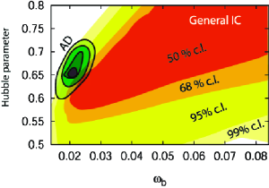
Figure 1: Joint Bayesian likelihood contours for the baryon density $\omega_{b}$ and the Hubble parameter $h$, using pre-WMAP CMB data only. The tighter contours (shades of green) assume purely AD initial conditions, the wider contours (yellow/shades of red) include general isocurvature IC (from Ref. TRD1 ).

Inclusion of general initial conditions in the analysis can lead to very important degeneracies in the IC parameter space, which spoil the accuracy with which other cosmological parameters can be measured by CMB alone. This has been demonstrated in a striking way for the case of the Hubble parameter and the baryon density in Ref TRD1 , cf Fig.  1. An effective way to break this degeneracy is achieved by the inclusion of large scale structure (LSS) data. The key point is that, once the corresponding CMB power spectrum amplitude has been COBE-normalized, the amplitude of the AD matter power spectrum is nearly two orders of magnitude larger than any of the isocurvature contribution (cf Fig.  2). Therefore the matter power spectrum essentially measures the adiabatic part, and is nearly insensitive to isocurvature contributions. The argument holds true for observations of the matter spectrum on all scales, ranging from large scale structure to weak lensing and Lyman $\alpha$-clouds. In view of optimally constraining the isocurvature content, it is therefore essential to combine those observations with CMB data, in order to break the strong degeneracy among initial conditions which is present in the CMB power spectrum alone Tprep .

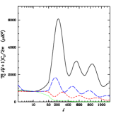
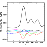
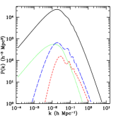
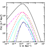
Figure 2: CMB (left) and matter (right) power spectra of the different auto- (odd panels) and cross-correlators (even panels) for the standard $\Lambda$CDM concordance model. The CMB power spectrum is COBE-normalized. The color and line style codes are as follows: in the odd panels, AD: solid/black line, CI: dotted/green line, NID: short-dashed/red line, NIV: long-dashed/blue line; in the even panels, AD: solid/black line (for comparison), $<{\rm AD},{\rm CI}>$: long-dashed/magenta line, $<{\rm AD},{\rm NID}>$: dotted/green line, $<{\rm AD},{\rm NIV}>$: short-dashed/red line, $<{\rm CI},{\rm NID}>$: dot-short dashed/blue line, $<{\rm CI},{\rm NIV}>$: dot-long dashed/light-blue line, and $<{\rm NID},{\rm NIV}>$: dot-short dashed/black line.

3 The cosmological constant and isocurvature IC

We apply the above statistical (Bayesian or frequentist) and physical (general initial conditions, matter power spectrum) considerations to the study of the cosmological constant problem from pre-WMAP data. We outline the method and the main results below (see Ref. TRD2 for more details) and comment at the end on the qualitative impact of the new WMAP data on those findings.

Our analysis makes use of the COBE, BOOMERanG and Archeops data CMBdata , covering the range $3\leq\ell\leq 1000$ in the CMB power spectrum. For the matter power spectrum, we use the galaxy-galaxy linear power spectrum from the 2dF data 2dFdata , and we assume that light traces mass up to a (scale independent) bias factor $b$, over which we maximise. The main focus being on the type of initial conditions, we restrict our analysis to only 3 cosmological parameters: the scalar spectral index, $n_{S}$, the cosmological constant $\Omega_{\Lambda}$ in units of the critical density and the Hubble parameter, $H_{0}=100\,h{\;\mathrm{km}}{\;\mathrm{s}^{-1}}{\;\mathrm{Mpc}^{-1}}$. We consider flat universes only and neglect gravitational waves.

When we set to zero the isocurvature modes, we recover the well-known results for purely AD perturbations. Because of the “geometrical degeneracy”, CMB alone cannot put very tight lower limits on $\Omega_{\Lambda}$ even if we allow only for flat universes. The degeneracy can be broken either by putting an external prior on $h$ or via the LSS spectrum, since $P_{\rm m}$ is mainly sensitive to the shape parameter $\Gamma\equiv\Omega_{\rm m}h$. Combination of CMB and LSS data yields the following likelihood (Bayesian) intervals for $\Omega_{\Lambda}$:

$$\Omega_{\Lambda}=0.70_{-0.05}^{+0.05}\mbox{ at $1\sigma$ $\quad$ and $\quad$}_{-0.27}^{+0.15}\mbox{ at $3\sigma$}.$$ (1)

From the Bayesian analysis, one concludes that CMB and LSS together with purely AD initial conditions require a non-zero cosmological constant at very high significance, more than $7\sigma$ for the points in our grid! However, our best fit has a reduced chi-square $\chi/F=0.59$, significantly less than $1$. This leads to artificially tight likelihood regions: the observationally excluded part of parameter space is less extended, and is given by the frequentist analysis. From the frequentist approach, we obtain instead the following confidence intervals:

$$0.15<\Omega_{\Lambda}<0.90\mbox{ at $1\sigma$ $\quad$ and $\quad$}\Omega_{\Lambda}<0.92\mbox{ at $3\sigma$}.$$ (2)

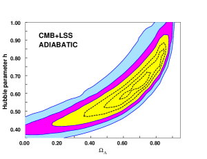
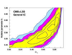
Figure 3: Bayesian (dashed lines) and frequentist (solid, filled) joint $1\sigma$, $2\sigma$, $3\sigma$ contours using pre-WMAP CMB and 2dF data. The left panel assumes purely adiabatic IC, the right panel includes general isocurvature IC.

When we enlarge the space of models by including all possible isocurvature modes, likelihood (Bayesian) and confidence (frequentist) contours widen up along the $\Omega_{\Lambda}$, $h$ degeneracy, and this produces a considerable worsening of the likelihood limits. For general initial conditions we now find (Bayesian, CMB and LSS together):

$$\Omega_{\Lambda}=0.70_{-0.10}^{+0.15}\mbox{ at $1\sigma$ $\quad$ and $\quad$}_{-0.48}^{+0.25}\mbox{ at $3\sigma$}.$$ (3)

Again, the frequentist statistics give less tight bounds:

$$\Omega_{\Lambda}<0.90\mbox{ at $1\sigma$ $\quad$ and $\quad$}\Omega_{\Lambda}<0.95\mbox{ at $3\sigma$},$$ (4)

and in particular we cannot place any lower limit on the value of the cosmological constant. A complete discussion can be found in Ref. TRD2 . Joint likelihood contours for $\Omega_{\Lambda}$, $h$ with AD and general isocurvature initial conditions are plotted in Fig. 3 for both statistical approaches.

From the frequentist point of view, the region in the $\Omega_{\Lambda},h$ plane which is incompatible with data at more than $3\sigma$ is nearly independent on the choice of initial conditions (compare left and right panel of Fig. 3). Enlarging the space of initial conditions seemingly does not have a relevant benefit on fitting pre-WMAP data with or without a cosmological constant. In Fig. 4 we plot the best fit model (which has $\chi/F=0.67$) with general initial conditions and $\Omega_{\Lambda}=0$. As a consequence of the red spectral index ($n_{S}=0.80$) and of the absence of the early Integrated Sachs-Wolfe effect (since $\Omega_{\Lambda}=0$), the best fit model has a very low first acoustic peak, even in the presence of isocurvature modes. This is compatible with the BOOMERanG and Archeops data only if the absolute calibration of the experiments is reduced by $28\%$ and $12\%$, respectively. Furthermore, this best fit model has a rather low value of the Hubble parameter, $h=0.35$, which is many sigmas away from the value obtained by the HST Key Project, namely $h=0.72\pm 0.08$ HST . We conclude that a good fit to the pre-WMAP CMB data combined with LSS measurements can only be obtained at the price of pushing hard the other parameters, even when general initial conditions are allowed for.

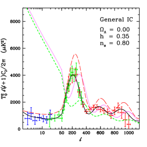
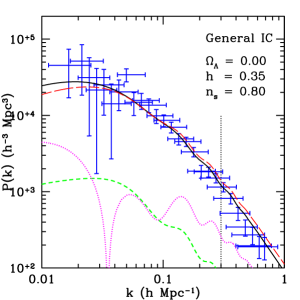
Figure 4: Best fit with general IC and $\Omega_{\Lambda}=0$, combining pre-WMAP CMB (left) and 2dF (right) data. In both panels solid/black is the total spectrum, long-dashed/red the purely AD contribution, short-dashed/green the sum of the pure isocurvature modes, dotted/magenta the sum of the correlators (multiplied by $-1$ in the left panel and in absolute value in the right panel).

Finally, in order to constrain deviations from perfect adiabaticity, it is interesting to limit quantitatively the isocurvature contribution. To this end, one can phenomenologically quantify the isocurvature contribution to the CMB power by a parameter $0\leq\beta\leq 1$, defined in Ref. TRD2 , so that purely AD IC are characterized by $\beta=0$, while purely isocurvature IC correspond to $\beta=1$. In Fig. 5 we plot the value of $\beta$ for the best fit models, with the frequentist exclusion regions superimposed. Within $2\sigma$ c.l. (frequentist), the isocurvature contribution to the IC is bounded to be less then $40\%$.

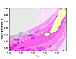
Figure 5: Isocurvature content $0.0\leq\beta\leq 1.0$ of best fit models with pre-WMAP CMB and 2dF data. The contours are for $\beta=0.20,0.40,0.60,0.80$ from the center to the outside. Shaded regions represents 1 to 3 $\sigma$ c.l..

Although a quantitative analysis using the more precise WMAP data has not yet been carried out, some qualitative features of the expected results can be discussed. In particular, the first peak has been measured by WMAP to be 10% higher then in previous observations WMAP . On the other hand, our work indicates that the first peak is very suppressed even in the presence of general IC for $\Omega_{\Lambda}=0$. Therefore one expects that WMAP data will exclude with much higher confidence a vanishing cosmological constant. In fact, our pre-WMAP best fit $\Omega_{\Lambda}=0$ model, when compared to the WMAP data WMAP , has $\chi^{2}_{WMAP}/F\approx 4.4$, and is therefore found to be totally incompatible with the new data. Furthermore, the constraints on non-adiabatic contributions should improve considerably, especially in view of the inclusion of polarization data BMTpol .

4 Conclusions

We have shown that the statistical approach (Bayesian or frequentist) can have an important impact in the determination of errors from CMB and LSS data. We found that structure formation data tend to prefer a non-zero cosmological constant even if general isocurvature initial conditions are allowed for. The isocurvature contribution is constrained to be $\leq 40\%$ at $2\sigma$ c.l. (frequentist).

Aknowledgments

It is a pleasure to thank Alessandro Melchiorri and all the organizers of the workshop. I am also grateful to Alain Riazuelo and Ruth Durrer for a most pleasant collaboration. RT is partially supported by the Schmidheiny Foundation, the Swiss National Science Foundation and the European Network CMBNET.

References

- (1) G.J. Feldman and R.D. Cousins, Phys. Rev. D 57, 3873-3889 (1998); A.G. Frodesen, O. Skjeggestad and H. Tofte, Probability and Statistics in Particle Physics (Universitetsforlaget, Bergen-Oslo-Tromso 1979); M.G. Kendall, and A. Stuart, The advanced theory of statistics, Vol. 2, 4th ed. (High Wycombe, London, 1977).
- (2) L. Page et al., preprint astro-ph/0302220 (2003).
- (3) M. Bucher, K. Moodley, and N. Turok, Phys. Rev. D 62, 083508 (2000).
- (4) R. Trotta, A. Riazuelo, and R. Durrer, Phys. Rev. Lett. 87, 231301 (2001).
- (5) R. Trotta, A. Riazuelo, and R. Durrer, Phys. Rev. D 67, 063520 (2003).
- (6) R. Trotta et al., in preparation.
- (7) G.F. Smoot et al., ApJ 396, L1 (1992); C.L. Bennett et al., ApJ 430, 423 (1994); M. Tegmark and A.J.S. Hamilton, in 18th Texas Symposium on relativistic astrophysics and cosmology, edited by A.V. Olinto et al., pp 270 (World Scientific, Singapore, 1997); C.B. Netterfield et al., ApJ 571, 604 (2002); A. Benoît et al., preprint astro-ph/0210306.
- (8) M. Tegmark, A. Hamilton and Y. Xu, Month. Not. R. Astron. Soc. (accepted), preprint astro-ph/0111575 (2001).
- (9) W. Freedman et al., ApJ 553, 47 (2001).
- (10) G. Hinshaw et al., preprint astro-ph/0302217 (2003); L. Verde et al., preprint astro-ph/0302218 (2003); A. Kogut et al., preprint astro-ph/0302213 (2003).
- (11) M. Bucher, K. Moodley, and N. Turok, Phys. Rev. Lett. 87, 191301 (2001); M. Bucher, K. Moodley, and N. Turok, Phys. Rev. D 66, 023528 (2002).