A VLT spectroscopic study of the ultracompact H ii region G29.96$-$0.02

A high quality, medium-resolution K-band spectrum has been obtained of the ultracompact H ii region G29.96$-$0.02 with the Very Large Telescope (VLT). The slit was positioned along the symmetry axis of the cometary shaped nebula. Besides the spectrum of the embedded ionizing O star, the long-slit observation revealed the rich emission-line spectrum produced by the ionized nebula with sub-arcsec spatial resolution. The nebular spectrum includes Br$\gamma$, several helium emission lines and a molecular hydrogen line. A detailed analysis is presented of the variation in strength, velocity and width of the nebular emission lines along the slit. The results are consistent with previous observations, but the much better spatial resolution allows a critical evaluation of models explaining the cometary shape of the nebula. Our observations support neither the wind bow shock model nor the champagne flow model.
The measured line ratios of the nebular hydrogen and helium lines are compared to predictions from case B recombination-line theory. The results indicate an electron temperature between 6400 and 7500 K, in good agreement with other determinations and the Galactocentric distance of 4.6 kpc. The He⁺/H⁺ ratio is practically constant over the slit; we argue that He is singly ionized throughout the nebula. We review the various observational constraints on the effective temperature of the ionizing star and show that these are in agreement with its K-band spectral type of O5–O6 V.

1 Introduction

H ii regions trace the formation sites of massive stars. The ionizing radiation of the embedded, young OB stars is absorbed by gas and dust in their near surroundings and re-emitted at infrared and radio wavelengths. Their progenitors, the ultracompact H ii (UCHii) regions, represent the earliest recognizable phase of massive-star formation, and are the most luminous sources at 100 $\mu$m, observable throughout the Galaxy (Churchwell, 1990; Garay & Lizano, 1999). The small size and large number of UCHii regions indicate that the lifetime of this phase is significantly longer than the $\sim 10^{4}$ year predicted by models describing the expansion of young H ii regions.

A possible solution for this “confinement problem” is suggested by the observed morphologies of UCHii regions. The frequently seen cometary structures are suggestive of bow shocks. Wood & Churchwell (1989) proposed that these bow shocks might result from the supersonic motion ($v_{\rm sound}\simeq 1$  km s^-1) of the embedded O stars relative to the ambient molecular cloud. The stand-off distance of the shock, and thus the observed “size” of the UCHii regions, is determined by the density of the ambient medium, the velocity of the O star, and the momentum of its stellar wind. These parameters are not expected to vary rapidly with time, thus delaying the apparent expansion rate of the UCHii region (e.g. van Buren et al., 1990; Mac Low et al., 1991; van Buren & Mac Low, 1992).

G29.96$-$0.02, also denominated IRAS 18434$-$0242 (hereafter G29.96), is a well-studied, cometary-shaped UCHii region at a Galactocentric distance of 4.6 kpc (e.g. Pratap et al., 1999). Arguments based on extinction and the spectral type of the ionizing star favour the near heliocentric distance of 6 kpc instead of the far distance of 9 kpc (Pratap et al., 1999). The cometary structure of G29.96 was first observed by Wood & Churchwell (1989) at radio wavelengths. Follow-up radio observations were performed by Wood & Churchwell (1991), Afflerbach et al. (1994), Cesaroni et al. (1994), Fey et al. (1995) and Kim & Koo (2001). The cometary shape is characterized by a sharp, bright, arc-like leading edge and a low-surface brightness tail of emission which trails off away from the edge. Wood & Churchwell (1989) found the bow shock hypothesis consistent with their radio recombination line observations of G29.96. Alternatively, a champagne-flow model, which describes the spherical expansion of an H ii region into a molecular medium with a steep density gradient (Yorke, 1986), has been proposed to explain the morphology and kinematical structure of G29.96 (Lumsden & Hoare, 1996, 1999).

G29.96 is embedded in a molecular cloud that produces $\sim 15$ magnitudes of visual extinction (see Martín-Hernández et al., 2002a). This molecular cloud has been extensively studied at low spatial resolution (Churchwell et al., 1990, 1992). Strong emission from different dense gas tracers indicates the presence of hot, dense gas. Just in front of the edge of the H ii region, at approximately 2″ west of the radio continuum peak, a hot molecular core was discovered in interferometric observations (Cesaroni et al., 1994, 1998; Maxia et al., 2001). Recently, this hot core has been found at mid-infrared wavelengths too (De Buizer et al., 2002). The observed offset between the hot core and the H ii region and the detection of masers towards the core (Pratap et al., 1994; Hofner & Churchwell, 1996; Walsh et al., 1998) suggest that the hot core is not heated by the ionizing star of G29.96, but by another young, deeply embedded massive star.

G29.96 seems to be associated with a small cluster of stars (Fey et al., 1995; Lumsden & Hoare, 1996; Watson et al., 1997; Pratap et al., 1999). The main ionizing star is located in the focus of the bright arc. Watson & Hanson (1997) obtained a K-band spectrum of the embedded ionizing star, the first ionizing star of an UCHii region ever detected. Based upon the presence and strength of photospheric lines of C iv and N iii, they deduced a main sequence spectral type between O5 and O8.

G29.96 provides an excellent laboratory to test models describing the ionization structure of an UCHii region. The ionization structure can be traced by the nebular hydrogen and helium recombination lines. The comparison between observations and model provides an important constraint on the stellar parameters of the ionizing star(s), yielding important information on the properties of newly formed massive stars (e.g. Vanzi et al., 1996; Lumsden & Puxley, 1996; Lumsden et al., 2001a; Hanson et al., 2002). Due to the large visual extinction towards H ii regions like G29.96, such a study has only recently become possible thanks to the technological development of near-IR spectrometers.

In this paper we present new, high quality, long-slit K-band spectra of G29.96 (2.07–2.19 ${\rm\,\mu m}$). Besides Br$\gamma$, a large number of He i lines and a H₂ line are covered. The study of the relative strengths of the H i and He i lines as a function of position along the slit allows different lines of investigation. First, it is possible to study the impact of large line opacities on the He i lines. Second, the conditions present in the ionized gas can be determined. Third, the results constrain the effective temperature of the ionizing star, which can be compared with the spectral type implied by its K-band spectrum. Finally, the kinematical structure of the ionized gas can be studied at higher spatial resolution than in previous studies (Wood & Churchwell, 1991; Afflerbach et al., 1994; Lumsden & Hoare, 1996, 1999) and compared with the molecular gas motions. This comparison can be used to test the different models (bow shock, champagne flow, etc.) that have been proposed to explain the cometary morphology of G29.96.

Figure 1: Acquisition image of the UCHii region G29.96–0.02 obtained through a narrow-band H₂ 1–0 S(1) filter (central wavelength 2.13 ${\rm\,\mu m}$). Coordinates are relative to the position of the ionizing star: $\alpha(2000)=18^{\rm h}46^{\rm m}4\aas@@fstack{s}075,\delta(2000)=-2\degr 39\arcmin 21\aas@@fstack{\prime\prime}42$. Contours are 1, 2.5, 5, 10, 25, 50, 75 and 90% the peak flux. The cometary structure of the H ii region is clearly revealed. The position of the slit is marked by a dashed line. The ionizing star and the bright arc are indicated. At a distance of 6 kpc, 1 arcsec corresponds to 0.029 pc.

This paper is structured as follows. Section 2 describes the observations and the data reduction. Section 3 presents the resulting spectra and the variations and kinematics of the lines across G29.96. Section 4 describes the H i and He i recombination theory and shows the different applications of these lines. Section 5 reviews the various observational constraints on the effective temperature of the ionizing star. Section 6 discusses the dynamics of G29.96. Finally, Sect. 7 summarizes the results of the paper.

2 Observations

Long-slit (120″) K-band spectra were obtained of the UCHii region G29.96 with ISAAC mounted on Antu (UT1) of ESO’s Very Large Telescope (VLT), Paranal, Chile. The observations were carried out on 19 March 2000. A slit-width of 0$\aas@@fstack{\prime\prime}$3 was used, resulting in a spectral resolving power R$\sim 8000$ ($=$c/$\Delta$v). The slit was positioned along the symmetry axis of the object (116.2 degrees with respect to the north-south axis). Figure 1 shows the location of the slit in the (acquisition) image of G29.96 obtained through a narrow-band H₂ filter (central wavelength 2.13 ${\rm\,\mu m}$).

The observing conditions at Paranal Observatory were excellent (humidity less than 10% and seeing of 0$\aas@@fstack{\prime\prime}$6). In order to correct for the sky background, the object was “nodded” between two positions on the slit (A and B) such that the background emission registered at position B (when the source is at position A) is subtracted from the source plus sky background observation at position B in the next frame, and vice versa. This strategy has the advantage that observing time is very efficiently used, but it reduces the effective length of the slit by about 50%; for G29.96 this is not a problem.

The electrical ghosts and bias were removed from the frames before flatfielding. Subsequently, the sky background emission was subtracted following the procedure outlined above. Wavelength calibration was performed using the telluric OH lines. The accuracy of the wavelength calibration is 3  km s^-1. To correct for absorption lines due to the Earth’s atmosphere, the target spectra were divided by the spectrum of a telluric standard star. For this purpose, an A-type star was observed under identical sky conditions, which provides a continuous spectrum only containing telluric absorption lines. The hydrogen Br$\gamma$ line in the A-star spectrum was removed by a model fit. The telluric standard was also used to correct for the throughput of telescope and instrument. For a more detailed description of the data reduction procedures we refer to Bik et al. (in preparation).

Spectra were extracted along the slit (1 pixel = 0$\aas@@fstack{\prime\prime}$147) in the spatial direction. The peak positions, equivalent widths and fluxes of the lines were measured by fitting a Voigt profile. A line is defined as being detected if its peak intensity exceeds the rms noise level of the local continuum by at least a factor three. The central wavelength of the line was measured with respect to the local standard of rest, i.e. corrected for the projected velocity of the Earth with respect to the Sun at the time of observation and for the solar motion in the direction of G29.96 ($v_{\rm LSR}=44$  km s^-1).

Figure 2: Nebular spectrum of G29.96–0.02 extracted from a 0$\aas@@fstack{\prime\prime}$3 $\times$ 0$\aas@@fstack{\prime\prime}$882 region around the peak of ionized emission. The lines observed, their identification and their relative flux with respect to Br$\gamma$ are listed in Table 1. Note the logarithmic scale of the flux scale.

Table 1: Emission lines in the nebular K-band spectra of G29.96$-$0.02.

$\lambda^{\dagger}$ (${\rm\,\mu m}$)	Identification	Peak flux◇		$\lambda^{\dagger}$ (${\rm\,\mu m}$)	Identification	Peak flux◇
2.10213♭	?	0.004		2.16147	He 73F–43D	0.024
2.11282	He 43S–33P	0.041		2.16240	He 71F–41D	0.007
2.11371	He 41S–31P	0.011		2.16495	He 71,3G–41,3F	0.046
2.12183	H2 1–0 S(1)	0.005		2.16612	H 7–4 (Br$\gamma$)	1.00
2.14570	[Fe iii] 3G3–3H4	0.009		2.18245	He 73P–43D	0.005
2.15007	He 73S–43P	0.002		2.18483	He 71D–41P	0.001

(^†) Vacuum wavelength. The vaccum rest wavelength for the H₂ line is taken from Bragg et al. (1982) and those of the He i lines from Benjamin et al. (1999). (^◇) Flux with respect to Br$\gamma$ at the position of the arc peak. (^♭) Observed line center wavelength.

Figure 3: Spatial variation of a) Br$\gamma$ , b–e) the strongest He i recombination lines and f) H₂ 1–0 S(1) across the symmetry axis of G29.96 (from left to right in Fig. 1). The normalized He i and H₂ intensity distributions are compared to the Br$\gamma$ profile (dashed line). The origin corresponds to the position of the ionizing star. At a distance of 6 kpc, 1″ corresponds to 0.029 pc. While the He i and H i distributions trace each other very well, the H₂ line peaks 0$\aas@@fstack{\prime\prime}$93 ahead of Br$\gamma$ and shows a different structure in the tail. We note that it was not possible to measure line fluxes close to the position of the ionizing star, which explains the absence of points in between $-1$″ and 0″.

Figure 4: Spatial variation of the velocity centroid (top panel) and line FWHM (bottom panel) of Br$\gamma$ and H₂ along the symmetry axis of G29.96 (from left to right in Fig. 1). Typical error bars are indicated at different positions along the slit. In panels a) and c), the intensity distribution of Br$\gamma$ is plotted (dashed line) for comparison. The dotted lines in panels b) and d) represent the average H₂ centroid velocity and FWHM calculated between positions $-3$″ and $+5$″, and $0$″ and $+5$″, respectively. The zero point along the slit corresponds to the position of the ionizing star. At a distance of 6 kpc, 1″ corresponds to 0.029 pc.

3 Results

Figure 2 shows the nebular spectrum of G29.96 extracted from a 0$\aas@@fstack{\prime\prime}$3 $\times$ 0$\aas@@fstack{\prime\prime}$882 region around the peak of the emission. The strongest line corresponds to Br$\gamma$. The detected He i emission lines are the transitions of 4³S–3³P at 2.1128 ${\rm\,\mu m}$, 4¹S–3¹P at 2.1137 ${\rm\,\mu m}$, 7³S–4³P at 2.1501 ${\rm\,\mu m}$, 7³F–4³D at 2.1615 ${\rm\,\mu m}$, 7¹F–4¹D at 2.1624 ${\rm\,\mu m}$, the 7^1,3G–4^1,3F blend at 2.1649 ${\rm\,\mu m}$ and the transitions of 7³P–4³D and 7¹D–4¹P at 2.1824 and 2.1848 ${\rm\,\mu m}$, respectively. From these He i lines, significant emission along the slit was found for the transitions of 4³S–3³P at 2.1128 ${\rm\,\mu m}$, 4¹S–3¹P at 2.1137 ${\rm\,\mu m}$, 7³F–4³D at 2.1615 ${\rm\,\mu m}$ and the 7^1,3G–4^1,3F blend at 2.1649 ${\rm\,\mu m}$. The 1–0 S(1) transition of H₂ at 2.1218 ${\rm\,\mu m}$ and the forbidden line of [Fe iii] at 2.1457 ${\rm\,\mu m}$ are also evident. Table 1 lists the observed lines with their identifications and their fluxes relative to that of Br$\gamma$ at the peak position. An unidentified feature is present at 2.1022 ${\rm\,\mu m}$. This feature has also been detected in near-infrared spectra of compact planetary nebula (Lumsden et al., 2001b).

We could measure the nebular line emission along $\sim 20$″ of the slit, centered on the position of the ionizing star. Figure 3 illustrates the spatial variation of the strongest lines in this region. Moving from right to left along the slit (see Fig. 1), the Br$\gamma$ flux (Fig. 3 a) slowly increases until the position of the star. After the star, the Br$\gamma$ flux rapidly reaches a maximum and subsequently decreases. This maximum is at 2$\aas@@fstack{\prime\prime}$27 ahead of the star and coincides with the arc observed at radio wavelengths (e.g. Wood & Churchwell, 1989). The peak corresponding to the arc is fitted by a Gaussian profile with a full width at half maximum (FWHM) of 1$\aas@@fstack{\prime\prime}$14. The global structure of the tail to the right of the star can be fitted by a semi-Gaussian centered at the position of the star and with a FWHM of 7$\aas@@fstack{\prime\prime}$1 and a height 0.21 times the peak flux. The following panels (b–f) in Fig. 3 compare the flux distribution of the strongest He i lines and the H₂ 2.1218 ${\rm\,\mu m}$ line to that of Br$\gamma$. The He i and Br$\gamma$ distributions trace each other very well, indicating that the zones of H⁺ and He⁺ are of roughly the same size. This indicates that the central ionizing star must be hot enough to produce ionized helium throughout the H ii region (see Sect. 4.2 for a detailed discussion). The variation in the H₂ line strength resembles the ionized gas profile well, although it displays some significant deviations. It peaks 0$\aas@@fstack{\prime\prime}$93 ahead of the Br$\gamma$ maximum and exhibits a different structure in the tail of G29.96. The H₂ peak corresponding to the arc can be fitted by a Gaussian profile with a FWHM of 0$\aas@@fstack{\prime\prime}$87. Since the spatial profiles of the H i, He i and H₂ lines have been obtained simultaneously in one same setting, the relative separation of the Br$\gamma$ and H₂ peaks is reliable.

The velocity structure of the ionized (as traced by, for instance, Br$\gamma$) and molecular gas (as traced by H₂) along the symmetry axis of G29.96 is shown in Fig. 4. Figure 4 a plots the centroid velocity of the Br$\gamma$ line along the central 20″ of the slit. There is a large variation in radial velocity ($\sim 38$ km s^-1) across the object. The gas in front of the head of the arc has a velocity which increases from 67 (position $-7$″) to 87  km s^-1 (position $-3$″). At the arc, between positions $-3$″ and $-1$″, the velocity increases more rapidly, reaching a value of 99  km s^-1 at the position of the line intensity peak. It continues to increase towards the tail where it reaches 105  km s^-1 at approximately 3″ behind the star. Afterwards, the velocity drops to a value of approximately 94  km s^-1 at $\sim 5$″ behind the star.

Figure 4 c shows the behaviour of the Br$\gamma$ FWHM. As can be seen, there is a very rapid increase of the linewidth ahead of the line intensity peak, which gets up to $\sim 62$  km s^-1 wide. The Br$\gamma$ line is $\sim 42-46$  km s^-1 wide behind the arc.

This behaviour of the Br$\gamma$ line velocity across the symmetry axis of G29.96 agrees well with the radio recombination line studies of Wood & Churchwell (1991) and Afflerbach et al. (1994). Low spatial resolution observations of Br$\gamma$ have been presented by Lumsden & Hoare (1996, 1999). In contrast to their results, we see a larger variation in the peak velocity of the Br$\gamma$ line along the symmetry axis. In particular, the appreciable increase in velocity by more than 30  km s^-1 just ahead of the arc is not apparent from their study. This is likely due to the poorer spatial resolution of this earlier study combined with the steep increase in peak intensity towards the arc, which gets a high weight in their spatial averaging procedure.

Figure 5: Partial Grotrian energy-level diagram of the He i singlet and triplet transitions showing the infrared lines observed in the K-band spectrum of G29.96 (solid arrows), other important infrared lines (dotted arrows) and the strongest optical lines (dashed arrows). Note that the energy levels are not drawn to scale. The wavelengths of the infrared lines are indicated in ${\rm\,\mu m}$; those of the optical lines in Å. The wavelengths of the lines used in the present analysis are marked by a box.

The velocity structure observed for Br$\gamma$ is compared to that of the molecular gas traced by the H₂ 1–0 S(1) line (see Figs. 4 b and 4 d). There is little variation in the peak velocity of the H₂ line, which shows an almost constant value of 100  km s^-1 across G29.96 (calculated between positions $-3$″ and $+5$″, where the H₂ line emission is significant, i.e. above 3$\sigma$). The average velocity of 100  km s^-1 is consistent with the values (around 98  km s^-1) obtained from single dish observations of rotational transitions of CS (e.g. Churchwell et al., 1992; Bronfman et al., 1996; Olmi & Cesaroni, 1999) and NH₃ (e.g. Churchwell et al., 1990; Cesaroni et al., 1992). VLA measurements of ammonia by Cesaroni et al. (1994) resulted in a value of 98.7  km s^-1 towards the hot core detected just in front of the arc of G29.96. Thus, the H₂ gas is practically at rest with respect to the ambient medium. The H₂ FWHM shows a practically constant value of 33  km s^-1 in the interval [0″, $+$7″]. This FWHM is of the order of the spectral resolution, implying that the H₂ line is unresolved between these positions. Similarly to the case of the ionized gas, a significant increase of the FWHM up to $\sim 50$  km s^-1 is observed in front of the star.

The K-band spectral observations of G29.96 by Lumsden & Hoare (1999), although of much lower spatial resolution than ours, have about twice our spectral resolution ($\sim 18$  km s^-1). Their observations of the $1-0$ S(1) H₂ line show, as well, a very rapid increase in linewidth (from $\sim 20$ to 28  km s^-1 in their case) ahead of the arc. They were also able to discern small variations of the H₂ centroid velocity in the same direction as those of the ionized gas. This behaviour is, however, not evident from our data.

Comparing the Br$\gamma$ and H₂ velocity structure, we note that around the position of the ionizing star (between positions $-2$″ and $+3$″), the ionized gas is systematically redshifted relative to the molecular gas by a few (2–5)  km s^-1, whereas in the tail and ahead of the arc it becomes progressively more blueshifted. The increasing blueshift of the ionized gas in front of the arc coincides with the significant increase in the Br$\gamma$ and H₂ FWHM. This pattern has to be due to acceleration of the ionized gas along the line of sight.

4 The recombination lines

The nebular spectrum of G29.96 is dominated by recombination lines of hydrogen and helium. For most of the H i emission lines observed in nebulae, there are no radiative transfer problems; hence, the Case B approximation (Hummer & Storey, 1987), which assumes that the Lyman transitions are optically thick, reproduces well, apart from dust extinction, the observed nebular spectra. The recombination radiation of He i singlets is very similar to that of H i, and can also be approximated by the Case B treatment. In this case, by considering Case B it is assumed that the nebula has a large optical depth in transitions arising from the 1¹S level. However, the recombination cascade of the He i triplets can be modified by the fact that the 2³S level (see Fig. 5) is highly metastable. All recaptures to triplets eventually cascade down to the 2³S level. Depopulation of this level can only occur through photoionization, through collisional transitions to 2¹S and 2¹P, or through the forbidden 2³S–1¹S transition. The rates of these processes are small and hence, the population of the 2³S level is large; in turn, the optical depth of the lower n³P–2³S transitions is substantial. Moreover, the collisional transitions from 2³S to upper levels become significant and the emission from these levels is enhanced with respect to the predictions of a pure recombination model. Because of this interplay of collisional and radiative transfer effects, the triplet lines become sensitive to the density and optical depth.

Recently, Benjamin et al. (2002) have considered the effect of the optical depth of the 2³S level on the recombination spectrum of a spherically symmetric nebula. They used a model atom with individual levels up to $n=20$ and parameterized their calculations in terms of the line center optical depth of the 3³P–2³S 3890 Å line. A FORTRAN program to calculate emissivities of lines arising from levels with $n\leq 10$ over a large range of nebular conditions is available from Benjamin et al.

Figure 6: Optical depth correction factor, $f$, for the 2.1128 ${\rm\,\mu m}$ He i line as a function of the electron temperature for $\tau_{3890}$ between 0 and 100 and an electron density $n_{\rm e}$ = $10^{4}$ ${\rm cm^{-3}}$.

We use this program to estimate the Case B line fluxes of the He i lines observed in the spectrum of G29.96 and their possible enhancement due to collisional excitation from the 2³S level, or as a result of significant opacity in the n³P–2³S series.

Although Benjamin et al. (2002) include the collisional coupling between the triplet and singlet levels, they find that only the triplet lines arising from low levels show a noticeable enhancement in strength with respect to the zero optical depth case. From the triplet lines observed in the spectrum of G29.96, we find that the effect of the finite optical depth of the 2³S level is only evident in the transition of 4³S–3³P at 2.1128 ${\rm\,\mu m}$. Adopting the nomenclature by Benjamin et al. (2002), we define the optical depth correction factor $f_{\rm line}$($n_{\rm e}$,$T_{\rm e}$,$\tau_{3890}$)= $j$($n_{\rm e}$,$T_{\rm e}$,$\tau_{3890}$)/$j$($n_{\rm e}$,$T_{\rm e}$,0), i.e. the ratio of the line emissivity for optical depth $\tau_{3890}$ to the emissivity for zero optical depth. Figure 6 presents the variation of the optical depth correction factor for the 2.1128 ${\rm\,\mu m}$ line as a function of $\tau_{3890}$ and $T_{\rm e}$ for the case of a nebula with $n_{\rm e}$=$10^{4}$ ${\rm cm^{-3}}$.

The optical depth of the 3³P–2³S 3890 Å line in G29.96 can be roughly estimated. We have that $\tau_{3890}=n(2^{3}{\rm S})\sigma_{3890}R$, where $n(2^{3}{\rm S})$ is the density of atoms in the metastable state, $\sigma_{3890}$ is the cross section at the line center of the 3890 Å line and $R$ is the radius of the nebula. The relative population of the $2^{3}{\rm S}$ level depends on the local electron density and temperature, and can be estimated using equation 5 in Kingdon & Ferland (1995). Assuming an electron density of 2$\times 10^{4}$ ${\rm cm^{-3}}$ and an electron temperature of 6500 K (Afflerbach et al., 1994), we find that $n(2^{3}{\rm S})/n({\rm He}^{+})\sim 8\times 10^{-6}$ in the tail of G29.96. Equation 1 in Benjamin et al. (2002) gives that $\sigma_{3890}\sim 7\times 10^{-14}$ cm² for $T_{\rm e}$$=6500$ K and a turbulent velocity of 0 km s^-1. Assuming a helium abundance of 10% by number and a nebular radius of 7″ (see Sect. 3), which at a distance of 6 kpc corresponds to $\sim 0.20$ pc, we obtain $\tau_{3890}\gg 100$. Considering a turbulent velocity of 20  km s^-1 and a filling factor of 0.1, we obtain $\tau_{3890}\sim 80$. Hence, the 2.1128 ${\rm\,\mu m}$ line is expected to be enhanced (see Fig. 6) with respect to the pure recombination model.

It is illustrative at this point to use the relative strengths of the He i recombination lines to (1) determine how closely these lines follow the recombination theory and (2) study their dependence on the local nebular conditions. The ratio between any two He i lines is insensitive to the electron density, but can depend on the electron temperature.

4.1 The electron temperature

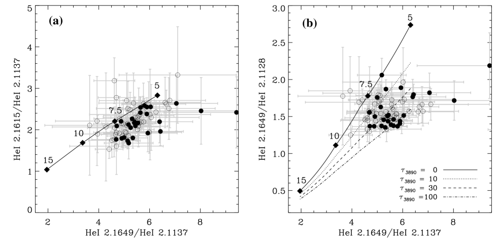
Figure 7: a) Plot of the line ratio 2.1615-7³F–4³D/2.1137-4¹S–3¹P against the ratio 2.1649-7^1,3G–4^1,3F/2.1137-4¹S–3¹P. Note that these line ratios should not depend on radiative transfer effects. b) 2.1649-7^1,3G–4^1,3F/2.1128-4³S–3³P against 2.1649-7^1,3G–4^1,3F/2.1138-4¹S–3¹P. In both figures, the solid line represents the Case B predictions for $T_{\rm e}$ = 5, 7.5, 10 and 15 $\times 10^{3}$ K (indicated by solid diamonds) and $n_{\rm e}$ $=10^{4}$ ${\rm cm^{-3}}$. The data indicate a temperature between 5000 and 7500 K. The non-solid lines in b) represent the calculations by Benjamin et al. (2002) for non-zero optical depth of the 2³S metastable level. Only points located in the interval [$-5$″, $+8$″] are considered. The data points from the tail of G29.96 ($>0$″) are plotted as open circles; those from the arc ($<0$″) are plotted as solid circles. The open and filled circles have very similar distributions.

Figure 7 a shows the relation between the He i line ratios 2.1615-7³F–4³D/2.1137-4¹S–3¹P and 2.1649-7^1,3G–4^1,3F/2.1137-4¹S–3¹P. These ratios show the largest dependence on $T_{\rm e}$. The calculations by Benjamin et al. (2002) show that these ratios are expected to be independent of radiative transfer problems arising from the metastable 2³S level. The solid line represents the theoretical predictions by Benjamin et al. (2002) for $T_{\rm e}$ = 5, 7.5, 10, 15 $\times 10^{3}$ K and $n_{\rm e}$ $=10^{4}$ ${\rm cm^{-3}}$. The model reproduces the trend in the data reasonably well, although there is a slight mismatch between data and theory. The data points are, on average, 20% below the model predictions. The origin of this discrepancy is unclear. It is clear from Fig. 7 a that the electron temperature of the ionized gas is in between 5000 and 7500 K, and that both the points from the tail of G29.96 ($>0$″) and those from the arc ($<0$″) are distributed equally.

Figure 7 b shows the relation between the He i line ratios 2.1649-7^1,3G–4^1,3F/2.1128-4³S–3³P and 2.1649-7^1,3G–4^1,3F/2.1137-4¹S–3¹P. The data show a significant spread in these line ratios, largely exceeding the quoted uncertainties. We conclude that the 2.1649/2.1128 ${\rm\,\mu m}$ line ratio is sensitive to the optical depth and that the 2.1128 ${\rm\,\mu m}$ line is enhanced with respect to the pure recombination case (solid line). A comparison with the model calculations (Benjamin et al., 2002) indicates optical depths, $\tau_{3890}$, in between 0 and 100, as expected (see above).

Figure 8: a) Electron temperature structure along the symmetry axis of G29.96 (from left to right in Fig. 1) as derived from the He i line ratio 2.1649/2.1138 ${\rm\,\mu m}$. The dashed line represents the average $T_{\rm e}$ of 6400 K. b) He⁺/H⁺ structure. The dashed line represents the average value of 0.087. Only points located in the interval [$-5$″, $+8$″] are considered.

A detailed electron temperature profile along the axis of G29.96 can be obtained by using the ratio of any two of the He i recombination lines. Figure 7 a shows that the 2.1649/2.1137 ${\rm\,\mu m}$ and 2.1615/2.1137 ${\rm\,\mu m}$ line ratios are reasonably well reproduced by the Case B approximation and can be used to probe variations in $T_{\rm e}$. Hence, by comparing the observed line ratios at any position with the Case B predictions we can measure the variation of $T_{\rm e}$ along the slit.

Figure 8 a shows the $T_{\rm e}$ profile along the symmetry axis of G29.96 as derived from the 2.1649/2.1137 ${\rm\,\mu m}$ line ratio. We see that the electron temperature is, within the uncertainties, constant along the slit with a mean value of 6400 $\pm$ 150 K. When we use the 2.1615/2.1137 ${\rm\,\mu m}$ line ratio, we also obtain a similarly constant $T_{\rm e}$ structure along the slit, but with a higher average value of 7550 $\pm$ 150 K. The difference between these two determinations comes from the discrepancy between data and theory shown in Fig. 7 a.

Our measurement of $T_{\rm e}$ is in good agreement with previous determinations. The non-LTE analysis of radio recombination line observations by Afflerbach et al. (1994) resulted in electron temperatures in between 6200 and 8600 K. They estimate an average $T_{\rm e}$ of $\sim 6500$ K. The electron temperatures derived by Wood & Churchwell (1991) from H76$\alpha$ recombination line observations towards G29.96 are low, ranging from $\sim 2500$ K in the tail to 4200 K in the arc. However, for this line, deviations from LTE can lead to temperature estimates lower than the true nebular temperature. Their best estimate of the electron temperature using non-LTE models is $\sim 5000$ K throughout the nebula. Finally, Watson et al. (1997) obtained temperatures in between 5000 and 7000 K over the nebula using 2, 6 and 21 cm continuum data.

Our estimate of $T_{\rm e}$ is also consistent with the Galactocentric distance of G29.96. The electron temperature in H ii regions has been shown to increase with the distance to the Galactic Center as a consequence of the decrease in metal content. This $T_{\rm e}$ gradient is approximately given by $T_{\rm e}$=5000+5000$\times$$R_{\rm Gal}$/15 (Shaver et al., 1983; Afflerbach et al., 1996; Deharveng et al., 2000). At the Galactocentric distance of G29.96 (4.6 kpc), the expected $T_{\rm e}$ is 6500 K, consistent with our value. This electron temperature corresponds to an enhancement of the metal content by a factor of $\sim 2$ with respect to that in the solar neighbourhood. This metallicity is in agreement with the analysis based on the infrared fine-structure lines observed towards G29.96 (see Martín-Hernández et al., 2002a).

4.2 He⁺/H⁺

The He⁺/H⁺ structure along the symmetry axis of G29.96 can be determined from the ratio of a singlet He i line to Br$\gamma$ once a specific model for the $T_{\rm e}$ structure of the H ii region has been assumed (such a ratio is insensitive to the electron density). The only singlet line we were able to measure along the slit is the transition of 4¹S–3¹P at 2.1137 ${\rm\,\mu m}$.

Figure 9 shows the relation between this ratio and the $T_{\rm e}$-indicator He i 2.1649/2.1137 ${\rm\,\mu m}$. There is an (anti)correlation between these two line ratios because of the different $T_{\rm e}$ dependence for the He i single/triplet and the H i lines. The observed data points are well matched by He⁺/H⁺ abundances in between 0.08 and 0.10 and electron temperatures in between 5000 and 7500 K. A preponderance of low He⁺/H⁺ abundances in the tail region is evident from this figure. This may reflect a He⁺ zone somewhat smaller than the H⁺ zone. Such a difference would be spatially more prominent in the low density tail.

The detailed He⁺/H⁺ structure along the symmetry axis of G29.96, calculated for $T_{\rm e}$ = 7000 K, is plotted in Fig. 8 b. We find that He⁺/H⁺ is practically constant across the slit. We obtain an average He⁺/H⁺ abundance of $0.087\pm 0.001$. Considering a total helium abundance by number of $\sim 0.1$, this implies that He is practically singly ionized throughout the nebula.

Kim & Koo (2001) estimated the value of He⁺/H⁺ at different positions in G29.96 from the ratio of the ratio of the radio recombination lines He76$\alpha$ and H76$\alpha$. They derived values in between 0.063 and 0.080, slightly lower than our estimate of 0.087. Their lower estimate could be due, however, to non-LTE effects on the radio recombination lines that may not have been taken into account, or to beam smearing.

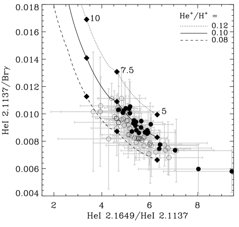
Figure 9: The line ratio He i 2.1649/Br$\gamma$ is plotted against the ratio He i 2.1649/2.1137. The lines represent the theoretical ratios for 3 different He⁺/H⁺ abundances (0.08, 0.10 and 0.12) and an electron density of $10^{4}$ ${\rm cm^{-3}}$. The values corresponding to $T_{\rm e}$ = 5, 7.5 and 10 $\times 10^{3}$ K are indicated by solid diamonds. As in previous figures, only points located in the interval [$-5$″, $+8$″] are considered, the data points in the tail of G29.96 are plotted as open circles and those from the arc as solid circles.

Figure 10: The relative extent of the He⁺ region to that of the H⁺ region, $R_{\rm He^{+}}/R_{\rm H^{+}}$, is plotted against $T_{\rm eff}$, the effective temperature of the ionizing star. For $T_{\rm eff}\geq 40\,000$ K, the He⁺ and H⁺ zones are coincident.

We have already mentioned in Sect. 3 that the central ionizing star in G29.96 must be hot enough to produce ionized helium throughout the H ii region. In order to investigate the dependence of the relative extent of the He⁺ region compared to that of the H⁺ region, $R_{\rm He^{+}}/R_{\rm H^{+}}$, on the effective temperature of the star, we have calculated a set of nebular models with the photoionization code CLOUDY version 94.00 (Ferland 2000) using MICE, the IDL interface for CLOUDY created by H. Spoon. We compute nebular models for a static, spherically symmetric, homogeneous gas distribution with one ionizing star in the center. An inner cavity with a radius equal to 10¹⁷ cm is set. Two different sets of stellar atmosphere models are taken to describe the spectral energy distribution (SED): the CoStar models by Schaerer & de Koter (1997) and the WM-Basic models by Pauldrach et al. (2001). We use stellar models for main sequence (dwarf) stars. The number of hydrogen ionizing photons emitted by the central source is fixed to that of the SED used, the metallicity of the nebula is set to twice solar and the density equal to 10⁴ ${\rm cm^{-3}}$, appropriate for G29.96 (Afflerbach et al., 1994; Wood & Churchwell, 1991).

Figure 10 shows $R_{\rm He^{+}}/R_{\rm H^{+}}$ as a function of the effective temperature of the star, $T_{\rm eff}$. It is seen that for $T_{\rm eff}\geq 40\,000$ K, the He⁺ and H⁺ zones are coincident, and that this result is independent of the SED used. Using the calibration by Vacca et al. (1996), this corresponds to a spectral type earlier than O7.5. This calibration is, however, based on plane-parallel models which do not incorporate stellar winds and line blocking/blanketing. A more recent calibration by Martins et al. (2002), based on non-LTE line blanketed atmosphere models with stellar winds computed with the cmfgen code of Hillier & Miller (1998), yields a spectral type equal to or earlier than O6. This spectral type determination is compared to estimates using other methods in Sect. 5.

5 The ionizing star of G29.96

The opening up of the infrared window has favoured in recent years the use of infrared spectra to infer the spectral type of the ionizing stars in heavily extincted regions. The first spectral classification in the K-band of a star ionizing an UCHii region was that of G29.96 (Watson & Hanson, 1997). The K-band classification (Hanson et al., 1996) is based on the presence and strength of photospheric lines of He i (2.058 and 2.1126 ${\rm\,\mu m}$), C iv (2.078 ${\rm\,\mu m}$), N iii (2.1155 ${\rm\,\mu m}$), H i (2.1661 ${\rm\,\mu m}$) and He ii (2.1885 ${\rm\,\mu m}$). The H i and He i lines, however, are heavily contaminated by nebular emission. Based on the other features, the spectral types that can be determined from the direct observation of the K-band spectrum are: O3–O4 (N iii  emission and He ii  absorption, but no C iv  emission), O5–O6.5 (both N iii  and C iv  emission and He ii  absorption), O7–O8 (N iii  emission and He ii  absorption, and weak C iv  emission), and O9 or later (none of these). Using this classification scheme, Watson & Hanson (1997) restricted the ionizing star in G29.96 to spectral type O5–O6.5.

Figure 11 shows the spectrum of the ionizing star of G29.96 extracted from the slit (Kaper et al. 2002; Bik et al. in prep.). The emission features of C iv  and N iii  are clearly present. The spectral coverage of our observations was not large enough to include the He ii  line at 2.1885 ${\rm\,\mu m}$. The presence and strength of the C iv  and N iii  features is consistent with the estimate by Watson & Hanson (1997), i.e. with an O5–O6.5 star. Watson & Hanson (1997) note that spectral types as late as O7–O8 could also be consistent with the data if the C iv  and N iii  features were enhanced as a consequence of G29.96 being a region with a metallicity twice that of the Sun. However, these late spectral types are ruled out because they are not hot enough to produce a He⁺ zone coincident with that of H⁺ (see Sect. 4.2). Thus, the K-band spectrum of the ionizing star, together with the condition imposed by the extent of the He⁺ zone (equal to or earlier than O6), limits the spectral type to O5–O6.

Table 2: Different estimates of the spectral type of the ionizing star in G29.96.

Method	$T_{\rm eff}$ (kK)	Spectral type△	Reference
Bolometric luminosity	$<49^{\dagger}$	$<$ O3⋆	1, 2
Lyman continuum photon flux	$35-40^{\dagger}$	O8 – O6⋆	3, 4, 5, 6, 7
Near-IR photometry	$\leq 42.5$	$\leq$ O5⋆	2
Nebular IR lines	32 – 38	O9 – O6.5⋆	8
Extent of the He+ zone	$\geq 40^{\sharp}$	$\geq$ O6♯	9
K-band spectrum	38 – 42.5⋆	O6.5 – O5	9,10

(^△) “$>$” means “earlier than”, and “$<$” means “later than”. (^†) Adopting the calibration by Vacca et al. (1996). (^⋆) Adopting the $T_{\rm eff}$ scale by Martins et al. (2002) for dwarf stars. (^♯) See Sect. 4.2. References: (1) Peeters et al. (2002); (2) Watson et al. (1997); (3) Wood & Churchwell (1989); (4) Cesaroni et al. (1994); (5) Becker et al. (1994); (6) Fey et al. (1995); (7) Kim & Koo (2001); (8) Morisset et al. (2002); (9) this work; (10) Watson & Hanson (1997);

Figure 11: Spectrum of the ionizing star in G29.96. The emission features of C iv at 2.080 ${\rm\,\mu m}$ and N iii at 2.116 ${\rm\,\mu m}$ are indicated. These features constitute the base of the K band classification. The lines of H i and He i are contaminated by nebular emission.

Various other estimates of the spectral type of the dominant ionizing star of G29.96 have been obtained from very different observations and methods. We briefly discuss these estimates using up-to-date stellar models and homogeneous assumptions. In particular, all observational constraints are scaled to a distance of 6 kpc and we use the latest temperature scale of O stars by Martins et al. (2002). We assume that the ionizing star is an unevolved zero age main sequence (ZAMS) star, although we note that some authors (Watson et al., 1997; Morisset et al., 2002) suggest that it may be a more evolved star. These estimates are (see also Table 2):

• Bolometric luminosity The total bolometric luminosity obtained from the IRAS fluxes (Peeters et al., 2002) and the overall SED (Watson et al., 1997) in an arcminute-sized region is log$(L/L_{\sun})=5.9$. Since this luminosity is integrated over a large region, it is likely to include contributions from other sources, for instance, the hot core. Hence, it must be considered as an upper limit to the bolometric luminosity of the ionizing star. This upper limit to the luminosity corresponds to a star with an effective temperature lower than 49 000 K (Vacca et al., 1996). Adopting the $T_{\rm eff}$-spectral type calibration by Martins et al. (2002) for dwarf stars, this corresponds to a star later than O3.

• Number of Lyman continuum photons The number of Lyman continuum photons derived for G29.96 from radio continuum observations is in the range log$(N_{\rm Lyc})=48.43-48.93$ s^-1 (Wood & Churchwell, 1989; Cesaroni et al., 1994; Becker et al., 1994; Fey et al., 1995; Kim & Koo, 2001), which corresponds to an effective temperature in between 35 000 and 40 000 K (Vacca et al., 1996). This $T_{\rm eff}$ range corresponds to a star with a spectral type of O8–O6 (Martins et al., 2002).

• Near-infrared photometry Constraints on the K magnitude and the bolometric luminosity allowed Watson et al. (1997) to place limits on the location of the ionizing star in the H-R diagram. They found a 3$\sigma$ upper limit on the effective temperature of 42 500 K. Adopting the $T_{\rm eff}$-spectral type calibration by Martins et al. (2002), this corresponds to a star equal to or later than O5.

• Nebular infrared lines The ratios of nebular fine-structure lines ([Ar iii]/[Ar ii] 9.0/7.0, [S iv]/[S iii] 10.5/18.7, [Ne iii]/[Ne ii]15.5/12.8 and [N iii]/[N ii] 57/128 ${\rm\,\mu m}$) observed by ISO (Peeters et al., 2002) have been used by Morisset et al. (2002) to constraint the properties of the ionizing star in G29.96. They use the most recent non-LTE line blanketed atmospheres with stellar winds and obtain effective temperatures in the range 32 000–38 000 K. Adopting the $T_{\rm eff}$-spectral type calibration by Martins et al. (2002), this corresponds to a star with a spectral type O6.5–O9.

Practically all the indirect methods to derive the spectral type which have been listed above agree well with the spectral type derived from the K-band spectrum. The exception is the method based on the nebular infrared lines, which predicts a slightly later type. In Martín-Hernández et al. (2002b) it was indicated that the infrared fine-structure line ratios such as [Ne iii]/[Ne ii] 15.5/12.8 ${\rm\,\mu m}$ are influenced by the stellar and nebular metallicity. Hence, their diagnostic use as indicator of the degree of ionization of the nebula is conditioned to an adequate treatment of the effect of metallicity on the stellar UV spectrum, i.e, on the line blocking/blanketing and stellar wind.

6 The dynamics of G29.96

Any model for the formation and evolution of the UCHii region G29.96 should be able to explain the following characteristics:

1. The general morphology of the nebula is described by a bright arc with the ionizing star in its focus and a lower surface brightness tail (see the 2 cm radio continuum image of Wood & Churchwell 1991, as well as the K-band image of Lumsden & Hoare 1996).

2. The molecular gas traced by H₂ shows a similar bright arc (see Fig. 1), but with the peak displaced ‘deeper’ into the molecular cloud (by 0$\aas@@fstack{\prime\prime}$93) than the ionized gas.

3. The ionized gas shows a steep gradient (see Fig. 4) which goes from $-31$  km s^-1 (just in front of the bright arc) to $+7$  km s^-1 (just behind the position of the star) relative to the molecular cloud velocity (which is about 98  km s^-1). The velocity then drops again to $-4$  km s^-1 in the tail.

4. In contrast with the large variations in velocity observed for Br$\gamma$ across the symmetry axis of G29.96, the H₂ emission shows no significant velocity gradients. Indeed, it seems to be at the velocity of the molecular cloud.

5. The FWHM of the Br$\gamma$ and H₂ lines are significantly higher in front of the respective bright arcs than in the tail. Specifically, the linewidths observed for Br$\gamma$ range from $42-46$  km s^-1 behind the star to values as high as 62  km s^-1 just in front of the arc. In the case of the H₂ line, the linewidth increases from 33  km s^-1 in the tail to $\sim 50$  km s^-1 in front of the H₂ arc.

Two different models aimed at explaining the formation and evolution of cometary H ii regions and applied to G29.9 appear in the literature: the bow shock model and the champagne flow model. Neither of these two models can account for all the characteristics observed for G29.96. We critically discuss both models.

6.1 The stellar bow shock model

The morphology of cometary H ii regions, in particular their near-parabolic shape, has been interpreted in terms of a bow shock (Wood & Churchwell, 1989). In such a model, an OB star moves with supersonic velocity (of a few  km s^-1) inside a molecular cloud. The interaction of the stellar wind with the ambient medium results in the formation of a bow shock with a cometary morphology. Detailed analytical and numerical models have been developed and applied to the UCHii region G29.96 (van Buren et al., 1990; Mac Low et al., 1991; van Buren & Mac Low, 1992).

The structure proposed by van Buren et al. (1990) of an UCHii region trapped in a bow shock is the following. The fast stellar wind (with a terminal velocity in excess of 2000  km s^-1) rams into the molecular cloud material, which is moving at supersonic velocity with respect to the star, resulting in the formation of a shock wave. The shock occurs at a radius where the momentum flux in the wind equals the ram pressure of the ambient medium. The immediate post-shock gas temperature is $\sim 10^{8}$ K. At this temperature, radiative cooling is not very efficient, but cooling via thermal conduction can lower the temperature very rapidly and consequently, this layer of shocked wind gas is rather thin (Comerón & Kaper, 1998). As the star moves through the ambient molecular medium, the hot bubble of shocked wind gas sweeps up material into a thin parabolic shell. Because of the rapid cooling, the wind only transfers its momentum to the swept-up shell in what is called a “momentum-driven” bow-shock. This shell traps all or part of the ionizing flux of the star, forming a thin layer of dense ionized gas surrounded by shocked molecular gas. The layer of ionized gas has the properties of a typical radiatively excited H ii region at a temperature of $\sim 10^{4}$ K.

In terms of the dynamics, the bow shock models essentially predict a redshift or blueshift of the ionized gas relative to the ambient cloud material depending on whether the star is moving away from the observer and into the molecular cloud, or towards the observer. The material in the bow shock is transported (due to a pressure gradient) from the head to the tail with a velocity that will not exceed the space velocity of the star by much. Note, however, that the material inside the bow shock flows in a direction away from the head to the tail, i.e. at some point it moves in a direction opposite from the stellar motion. The maximum velocity difference is then of the order of $v_{\star}\,{{\rm cos}(i)}$, where $v_{\star}$ is the relative velocity of the star through the ISM and $i$ is the inclination angle. As emphasized by Lumsden & Hoare (1996), the velocity structure observed for the Br$\gamma$ line can only be explained by the bow shock model if the molecular cloud velocity is 67  km s^-1, rather than the 98  km s^-1 obtained from rotational lines (e.g. Churchwell et al., 1990, 1992; Cesaroni et al., 1992; Bronfman et al., 1996; Olmi & Cesaroni, 1999). Moreover, if we attribute the difference of $\simeq 32$  km s^-1 observed in between positions $-7$″and 0″ (see Fig. 4 a) to the star-cloud interaction, then, with the inclination angle estimated from the morphology of $-45$ degrees (van Buren & Mac Low, 1992), this translates into a stellar velocity of $\simeq 45$  km s^-1. This is a very high velocity for a star in a cluster. Now, the difficulty with the stellar velocity might be mitigated if the velocity shoulder from 67 to 87  km s^-1 observed in Fig. 4 a between positions $-7$″ and $-3$″ traces motions in the hot core located just 2″ west of the bright arc. This hot core is known to have an embedded protostellar object with a prominent outflow (A. Gibb, private communication). In that case, the required molecular cloud velocity is 87  km s^-1 and the stellar velocity needed to explain the velocity difference between positions $-3$″and 0″ is only 17  km s^-1. However, still this velocity of 87  km s^-1 is much less than the observed molecular cloud velocity of 98  km s^-1.

The bow shock model provides a natural explanation for the general morphology of cometary H ii regions if the inclination angle is larger than $\pm 30$ degrees (Mac Low et al., 1991; van Buren & Mac Low, 1992). As an aside, we can test whether the morphology observed for G29.96 is consistent with that of an O5–O6 main sequence star (see Sect. 5) developing a bow shock. Van Buren et al. (1990) propose a simple analytical model for bow shocks in molecular clouds. The standoff distance $l_{\rm sd}$, i.e. the distance from the star where the momentum flux in the wind equals the ram pressure of the ambient medium, is given by:

$$l_{\rm sd}({\rm pc})=0.015\left({\dot{m}_{\star}\over{10^{-6}\,{\rm M}_{\sun}/{\rm yr}}}\right)^{1/2}\left({v_{\rm w}\over{10^{8}\,{\rm cm}/{\rm s}}}\right)^{1/2}$$

$$\left({n_{\rm H}\over{10^{5}\,{\rm cm}^{-3}}}\right)^{-1/2}\left({v_{\star}\over{10^{6}\,{\rm cm}/{\rm s}}}\right)^{-1}$$

where $\dot{m}_{\star}$ is the stellar wind mass-loss rate, $v_{\rm w}$ is the terminal velocity of the wind, $n_{\rm H}$ is the number density of hydrogen nuclei in all forms in the ambient gas and $v_{\star}$ is the relative velocity of the star through the ISM. We have adopted a mean mass per particle, $\mu_{\rm H}$, of 1.4 for the molecular gas. We take an O6 star with a metallicity twice solar (see Sect. 4.2) and stellar parameters adopted from Vacca et al. (1996). Following Vink et al. (2001), the corresponding stellar wind parameters are $\dot{m}_{\star}=2.81\times 10^{-6}$ M_☉ yr^-1 and $v_{\rm w}=2951$  km s^-1. A star of these characteristics moving supersonically trough the molecular cloud at a velocity of 17  km s^-1 will develop a bow shock with a standoff distance of 0.025 pc for a typical ambient gas density of $10^{5}$ ${\rm cm^{-3}}$. At a distance of 6 kpc and for an inclination angle of $-45$ degrees, this distance corresponds to a projected separation of 0$\aas@@fstack{\prime\prime}$6. From the observations (see Sect. 3), the projected standoff distance would be the offset between the star and the peak of the Br$\gamma$ arc, i.e. 2$\aas@@fstack{\prime\prime}$27. The observations imply either a much lower stellar velocity (of the order of 5  km s^-1) or a molecular gas density at the stagnation point below $10^{4}$ ${\rm cm^{-3}}$.

6.2 The champagne flow model

G29.96 has also been interpreted in terms of a champagne flow. Champagne flow (blister) models assume that the medium in which a massive star is born is not uniform but has strong density gradients, which can give rise to an H ii region that expands supersonically away from the high-density region in a so-called champagne flow (e.g. Tenorio-Tagle, 1979; Bodenheimer et al., 1979). Theoretical simulations of the expansion of an H ii region in the champagne phase, i.e. when the ionization front of the nebula crosses a region of strong density gradients, such as the edge of the molecular cloud, and expands into the lower density intercloud medium, have been presented by Yorke et al. (1983). During this champagne flow phase, the H ii region is ionization bounded on the high-density side (i.e. towards the molecular cloud) and density bounded on the side of the outward champagne flow.

The morphology of the ionized gas as predicted by these models is characterized by a bright compact component and an extended low brightness component roughly shaped like an opened fan. This compact component is inconsistent with the morphology observed for G29.96. At the same time, the opening of the morphology predicted for the tail region is not evident in G29.96.

In terms of the velocity structure, the numerical calculations (Yorke et al., 1983) show that the ionized gas is accelerated in the direction away from the molecular cloud to a relatively high velocity, which can attain values in excess of 30  km s^-1. On the contrary, very little variations should be observed near the core of the H ii region, where the ionization front should be essentially at the molecular cloud velocity (98  km s^-1 in the case of G29.96). However, we see it at 67  km s^-1 (or 87  km s^-1 if we attribute the velocity shoulder between position $-7$″ and $-3$″ to velocity flows within the hot core, see Sect. 6.1).

6.3 Final remarks

Neither of the two competing models can explain the observed velocity structure for G29.96. Partly, this may reflect the complex structure of this region, where the presence of a hot core with an embedded young stellar object and an associated outflow may obfuscate the dynamics.

Further progress will require the direct determination of the stellar velocity from photospheric absorption lines, for instance, from near-IR spectroscopy at high spectral resolution. We tried to obtain information on the stellar velocity from the C iv and N iii emission lines observed in our K-band spectrum, but it was not possible due to the complexity of these lines together with the limited spectral resolution ($\Delta{\rm v}\sim 33$  km s^-1). Also, a complete mapping of the dynamics of the ionized and molecular gas at both high spectral and spatial resolution will be essential.

A comparison of the observations with alternative models will also be important. Several authors, for instance, have investigated the interaction of a stellar wind and a clumpy molecular cloud material (e.g. Dyson et al., 1995; Redman et al., 1996; Williams et al., 1996). In this mass-loaded model, material from dense neutral clumps of gas is added to the ionized region around a newly formed massive stars; this neutral material soaks up ionizing photons, slowing down the expansion of the UCHii region. This mass-load model can explain cometary regions if the star is located in a density gradient of mass-loading clumps (Redman et al., 1998). G29.96 provides an excellent laboratory to test this model.

7 Summary

We presented a high quality, medium resolution K-band spectrum of the ultracompact region G29.96$-$0.02 obtained with the VLT. The slit was positioned along the symmetry axis of the nebula. Besides the spectrum of the embedded ionizing star, the observations included the emission-line spectrum produced by the ionized gas with sub-arcsec spatial resolution. The nebular spectrum includes Br$\gamma$, several helium emission lines, and a molecular hydrogen line.

The study of the relative strength of the Br$\gamma$ and He i lines as a function of position along the slit allowed us different lines of investigations. First, the observed helium lines in the nebula have been confronted with the He i recombination model. We have shown that the deviations of the transition of 4³S–3³P at 2.1128 ${\rm\,\mu m}$ from the Case B approximation are well described by the current understanding of the collisional and radiative transfer effects on the He i recombination spectrum of nebulae. The Case B approximation reproduces the ratios of He i lines originating from higher quantum states reasonably well. These He i line ratios indicate a constant electron temperature, between 6400 and 7500 K. Second, the relative strength of the Br$\gamma$ and the singlet transition of 4¹S–3¹P at 2.1137 ${\rm\,\mu m}$ indicates that He⁺/H⁺ is practically constant along the slit, with an average abundance of $0.087\pm 0.001$; we argue that He is singly ionized throughout the nebula. This conditions sets a lower limit to the effective temperature of the star.

The K-band spectrum of the ionizing star, together with the constraint imposed by the coincidence of the He⁺ and H⁺ zones, limit its spectral type to O5–O6. The various observational constraints on the effective temperature of the ionizing star are reviewed, and they are shown to be in rather good agreement with the above spectral type.

Finally, the variations in peak velocity and width of the Br$\gamma$ and H₂ lines allowed us to study the kinematical structure of the ionized and molecular gas at higher spatial resolution than in previous studies. We find that neither the wind bow shock model nor the champagne flow model are supported by the observations. A firm constraint on the velocity of the star and a complete mapping of the dynamics of the ionized and molecular gas at both high spectral and spatial resolution will be essential to understand the formation and evolution of G29.96.