Effects of Systematic Uncertainties on the Supernova Determination of Cosmological Parameters

Abstract

Mapping the recent expansion history of the universe offers the best hope for uncovering the characteristics of the dark energy believed to be responsible for the acceleration of the expansion. In determining cosmological and dark-energy parameters to the percent level, systematic uncertainties impose a floor on the accuracy more severe than the statistical measurement precision. We delineate the categorization, simulation, and understanding required to bound systematics for the specific case of the Type Ia supernova method. Using simulated data of forthcoming ground-based surveys and the proposed space-based SNAP mission we present Monte Carlo results for the residual uncertainties on the cosmological parameter determination. The tight systematics control with optical and near-infrared observations and the extended redshift reach allow a space survey to bound the systematics below 0.02 magnitudes at $z=1.7$. For a typical SNAP-like supernova survey, this keeps total errors within 15% of the statistical values and provides estimation of $\Omega_{m}$ to 0.03, $w_{0}$ to 0.07, and $w^{\prime}$ to 0.3; these can be further improved by incorporating complementary data.

1 Introduction

With the great increase in observational capabilities in the past and next few years, we can look forward to cosmological data of unprecedented volume and quality. These will be brought to bear on the outstanding questions of our “preposterous universe” [Carroll 2001] –what new forms of matter and energy constitute 95% of the universe? what is the underlying nature of the mysterious dark energy causing the observed acceleration of the expansion of the universe yet without an explanation within the standard model of particle physics? But more photons of any given observational method will not teach us the properties of the cosmological model before we understand the sources and intervening medium. Systematic uncertainties, rather than statistical errors, will bound our progress at the level where we fail to correct for astrophysical interference to our inference.

This applies to each one of the promising cosmological probes. Use of the cosmic microwave background radiation has been dramatically successful in fitting certain cosmological properties [Spergel et al. 2003], but others are tied up in degeneracies, insensitivities (e.g. to the dark energy equation of state behavior), and astrophysical foregrounds. Structure growth and evolution measures such as cluster counts by the Sunyaev-Zel’dovich effect or $X$-ray surveys and galaxy halo-density and velocity distributions through redshift surveys need to translate and disentangle observed quantities from theoretical ones, through problematic relations such as the mass-temperature law and the nonlinear matter power spectrum. Asphericities, clumpiness, bias, and foregrounds all play roles. Similar difficulties also apply to weak and strong gravitational lensing, Sunyaev-Zel’dovich measures of the angular diameter distance, peculiar velocity measurements, Alcock-Paczyński redshift distortions, etc. Certainly the Type Ia supernova method that discovered the acceleration of the universe [Perlmuter et al. 1999, Riess et al. 1998] is not exempt.

Type Ia supernova measurements have an advantage in a long track record of observations pushing the systematics to lower levels by understanding the astrophysical effects, making supplementary measurements, and correcting for the intervening quantities, reducing them to smaller residual uncertainties [Perlmutter & Schmidt 2003]. The quest for accurate cosmological parameter estimation at the percent level requires a well designed experiment dedicated to obtaining a systematics-bounded dataset. As we seek to pursue the supernova distance-redshift measurements to higher redshifts we gain from the increased discrimination between model parameters and from degeneracy breaking, but also require more stringent understanding and correction of systematics.

The level of accuracy required goes beyond treatment by simple analytic and Fisher matrix methods. While a rigorous treatment of the complexity of astrophysical observations –from detector pixel response to light-curve fitting to non-Gaussian and correlated errors– requires a well crafted end-to-end Monte Carlo simulation of the survey, this is perhaps overly detailed and model dependent to draw general conclusions.

In this paper we apply a more illustrative Monte Carlo method to broadly investigate the effects on cosmological parameter estimation –both errors and biases– due to systematic uncertainties and biases in the supernova magnitudes used in the Hubble diagram, or distance-redshift relation. Section 2 reviews the Hubble diagram. Section 3 considers the effect of an irreducible uncertainty in the form of both constant and redshift dependent magnitude systematics, while Section 4 examines the effect of a magnitude offset bias. The next three sections trace specific systematics through the supernova observations to the Hubble diagram and the cosmology fitting: Section 5 discusses calibration error, Section 6 selection effects (Malmquist bias), and Section 7 the magnitude de/amplification from gravitational lensing. Section 8 addresses methods for countering “evolution”, or population drift, through comprehensive use of spectral and flux time-series data.

For the Type Ia supernova method, this paper presents the basic analysis of the role of systematic errors and corrective measures in obtaining accurate as well as precise determinations of the cosmological parameters. Any cosmological probe or similar supernova survey must carry out such studies in order to quote parameter fitting capabilities with rigor. In the end, however, we will have a broad network of results, complementary and cross checking and thus synergistically powerful, that test the cosmological model and lead us toward understanding the fundamental physics responsible for our accelerating universe.

2 Tracing Cosmology with Supernovae

Type Ia supernovae have long been recognized as a powerful probe of cosmological dynamics, particularly in the measurement of its rate of expansion. In the SN Ia Hubble diagram, a plot of supernova peak magnitude versus redshift, the supernova brightness serves as a proxy for the supernova distance. The redshift $z=a^{-1}-1$ measures the scale factor $a$, the size of the universe when the supernova light was emitted relative to its current size. At low redshift, the data provide confirmation of a linear relationship between redshift and distance, the Hubble law. The dispersion of the data around the Hubble law measures how well supernova brightnesses serve as a proxy to distance. Studies of Type Ia Hubble diagrams have provided convincing evidence that SNe Ia can serve as standardizable candles, being able to determine luminosity distances to 5–10% [Phillips et al. 1999, Tripp & Branch 1999, Riess, Press & Kirshner 1996]. Models for SNe Ia must and do provide a simple theoretical explanation for this observational homogeneity [Höflich et al. 2003].

When considering distant supernovae, one should recognize that cosmological distances translate into a lookback time $t$ to when the supernova explosion occurred. Thus the distance-redshift measurement is also a mapping of the cosmic expansion history $a(t)$. At further lookback times (larger distances), secular deviations from the linear Hubble law, which represents a constant expansion rate, measure the acceleration or deceleration of the expansion of the universe. Fitting a set of cosmological parameters to the data in the Hubble diagram allows precise discrimination of different cosmological models, together with error estimation and confidence levels. This paper uses Monte Carlo and a flexible $\chi^{2}$-based cosmology fitter to simulate data from various distributions of supernovae, add statistical and systematic errors, and derive joint probability contours for the cosmological parameters.

The critical ingredients are the background cosmology model (§2.1), the supernova survey characteristics (§2.2), and the observational and astrophysical errors (§3–§7). Details of the fitting procedure are given in §2.3.

2.1 Cosmology

The luminosity distance to an object at redshift $z$ is given in terms of its comoving distance $r(z)$ by $d(z)=(1+z)\,r(z)$. Astronomers use magnitudes, a logarithmic measure of flux, which neglecting astrophysical effects like dust absorption, can be written as

$$m(z) = 5\log_{10}d(z)$$ (1)

$$+ \left[M+25-5\log_{10}\left(H_{0}/\left(100{\rm km/s/Mpc}\right)\right)\right]\ ,$$

where the distance $d(z)$ is made dimensionless by removing the Hubble scale $H_{0}^{-1}$, $M$ is the absolute magnitude of a supernova, and the constant in brackets is often notated $\cal M$. The influence of the cosmology resides in $d(z)$, or equivalently $r(z)$.

The comoving distance follows directly from the metric by

$$r(z)=\Omega_{k}^{-1/2}\sinh\left[\Omega_{k}^{1/2}\int_{0}^{z}dz^{\prime}/\left[H(z^{\prime})/H_{0}\right]\right],$$ (2)

where $\Omega_{k}=1-\Omega_{\rm tot}$, $\Omega_{\rm tot}$ is the total dimensionless energy density of the universe, $\sinh$ is analytically continued to $\sin$ for imaginary arguments, and $H(z)$ is the Hubble parameter. Since cosmic microwave background data strongly suggests our universe is flat, $\Omega_{k}=0$, we employ in the rest of this paper the appropriate limit,

$$r(z) = \int_{0}^{z}dz^{\prime}/\left[H(z^{\prime})/H_{0}\right]$$ (4)

$$= \int_{0}^{z}dz^{\prime}\left[\Omega_{m}(1+z^{\prime})^{3}\right.$$

$$\ \ \ \ \ \ \ +\ (1-\Omega_{m})e^{3\int_{0}^{z^{\prime}}\frac{dz^{\prime\prime}}{1+z^{\prime\prime}}\,(1+w(z^{\prime\prime}))}\left.\right]^{-1/2}.$$

Here $\Omega_{m}$ is the dimensionless matter density and $w(z)$ is the equation of state, or pressure to energy density ratio, of the other component – negative-pressure dark energy.

Two common parameterizations for the equation of state are $w=w_{0}+w_{1}z$ and $w=w_{0}+w_{a}(1-a)$, where $a$ is the scale factor of the universe. The exponential in (4) resolves respectively to $(1+z^{\prime})^{3(1+w_{0}-w_{1})}e^{3w_{1}z^{\prime}}$ and $(1+z^{\prime})^{3(1+w_{0}+w_{a})}e^{-3w_{a}z^{\prime}/(1+z^{\prime})}$. In either case we have a three-parameter phase space describing the cosmology: $\Omega_{m}$, $w_{0}$, $w^{\prime}$ (where the time variation $w^{\prime}$ is taken to be either $w_{1}$ or $w_{a}/2$; for purely historical reasons, we use $w_{1}$ in this paper). This covers the important quantities of the energy density, the dark-energy equation of state (EOS), and a measure of the physically revealing EOS time variation. In addition there is the nuisance parameter of the zero offset $\cal M$.

For a fiducial model we adopt in this paper (except in Fig. 5) a model with $\Omega_{m}=0.3$ in matter and $1-\Omega_{m}$ in a cosmological constant, $w=-1$ (that is, $w_{0}=-1$ and $w^{\prime}=0$). Section §2.3 contains a discussion of the effect of variation of the model. The parameters are allowed to range freely about the fiducial values. However, we do generally impose on the matter density a Gaussian prior $\sigma(\Omega_{m})=0.03$, reflecting anticipated information from other cosmological probes. While we believe that this is a reasonable assumption (there are recent studies [Allen, Schmidt & Fabian, 2002] that claim that a precision around $\sigma(\Omega_{m})=0.035$ has already been achieved), we have checked that relaxing this assumption to $\sigma(\Omega_{m})=0.05$ would roughly increase all uncertainties on $w^{\prime}$ given below by less than 50%, while leaving the other parameters unchanged (see also [Weller & Albrecht 2001]). Alternatively, a slightly more powerful constraint could have been obtained by including as a prior the projected measurement of the distance to the surface of last scattering by the Planck mission [Frieman et al. 2003].

2.2 Supernova Survey Characterization

The observations can be characterized in terms of the distribution in redshift of the supernova distance data and the dispersion about perfectly constant intrinsic peak flux (absolute magnitude) remaining after standardization for astrophysical and observational effects. For determining cosmological parameters, only the relative flux ratio between supernovae at different redshifts, not the absolute values, is important, thus the constant offset ${\cal M}$ composed of the absolute magnitude and the Hubble constant is just a nuisance parameter that needs to be integrated over.

One promising survey is the proposed Supernova/Acceleration Probe (SNAP) [SNAP 2003]. This involves a 2 meter telescope in space discovering and following some 2000 SNe Ia between $z=0.3-1.7$ with an optical/near infrared imager and spectrograph.

The magnitude dispersion of a given supernova is assumed to be constant and independent of redshift, for a well designed survey. We take it to be $\sigma_{m}=0.15$ for all surveys. This roughly corresponds to an intrinsic magnitude dispersion of 0.1 mag (or a 5% uncertainty in distance) and an equivalent statistical uncertainty in the determination of the corrected peak magnitude. The aggregated statistical error can be reduced by increasing the survey size to boost the number of supernovae. Note that at redshifts $z\mathrel{\mathchoice{\lower 3.6pt\vbox{\halign{$\mathsurround=0pt\displaystyle\hfil#\hfil$\cr<\crcr\sim\crcr}}}{\lower 3.6pt\vbox{\halign{$\mathsurround=0pt\textstyle\hfil#\hfil$\cr<\crcr\sim\crcr}}}{\lower 3.6pt\vbox{\halign{$\mathsurround=0pt\scriptstyle\hfil#\hfil$\cr<\crcr\sim\crcr}}}{\lower 3.6pt\vbox{\halign{$\mathsurround=0pt\scriptscriptstyle\hfil#\hfil$\cr<\crcr\sim\crcr}}}}0.8$ SNAP essentially follows all supernovae in the volume, so for these redshifts the sky area or survey lifetime would need to increase to gain statistics.

Since the sensitivity of the data to the cosmological parameters depends on redshift (for example at low redshift the distance reduces to $d=z$ for all cosmological models), the redshift distribution of the supernovae is important. The major effect is from the survey depth, $z_{max}$; optimization studies show the parameter estimations to be fairly insensitive to the exact distribution so long as the full redshift range is covered [Huterer & Turner 2001, Frieman et al. 2003]. Thus other observational and instrumental considerations can be taken into account for the distribution without harm to the science results.

Table 1: The redshift distribution $N(z)$ of the 2000 SNe employed from a fiducial SNAP survey. The redshifts $z$ given in the table correspond to the upper edges of each bin.

$z$	0.1	0.2	0.3	0.4	0.5	0.6	0.7	0.8	0.9	1.0	1.1	1.2	1.3	1.4	1.5	1.6	1.7
$N(z)$	0	35	64	95	124	150	171	183	179	170	155	142	130	119	107	94	80

For the space-based mission we adopt a fiducial distribution shown in Table 1, which we will call the SNAP distribution in the following. When considering shallower surveys we cut and rescale the SNAP distribution: truncating the SNAP distribution at the new $z_{max}$ and then multiplying $N(z)$ by the factor needed to keep the total number unchanged from the original, e.g. 2000 supernovae. This ensures that we can compare surveys based on their redshift reach, with their statistics on an equal footing. As we discuss in §3.1, the parameter estimation precision is not driven by statistics, i.e. numbers of supernovae, so we consider the total number fixed at 2000, well within the capabilities of SNAP. We have also checked that adopting instead a form $N(z)$ of some proposed ground-based survey affects the results by less than a few percent.

Additionally, in all cases we include a very low redshift (“local Hubble flow”) group of supernovae, 300 between $z=0.03-0.08$, such as will soon be available from the Nearby Supernova Factory [Aldering et al. 2002]. These prove important for marginalizing (averaging) over the extra parameter ${\cal M}$ to reduce the parameter phase space.

2.3 Cosmological Parameter Fitting

Given the elements of the previous two subsections, we can generate Monte Carlo realizations of supernova magnitude data vs. redshift, i.e. Hubble diagrams. These are then fit with the set of cosmological parameters using an unbinned $\chi^{2}$ minimization method. Two independent codes, one using the Minuit minimization package from the CERN library [Minuit 2002] and the other a CERN adaptation of a NAG routine [NAG 2002], have been checked against each other. Each generates the best fit to the data within the four dimensional parameter space $\{\Omega_{m},w_{0},w^{\prime},{{\cal M}}\}$ and the contours of 68% (or whatever level) confidence. The two-dimensional plots shown are marginalized over the other two parameters. In general the errors are non-Gaussian and asymmetric. Where numbers are quoted as $1\sigma$ errors, they refer to the 68% confidence level parabolic error on that parameter, marginalizing over the rest of the likelihood space.

Note that the error contours depend not only on the data errors but also on the background, fiducial cosmology. This is discussed and illustrated in §4. So in fact there is no unique parameter estimation precision associated with a given survey, even if the data properties, systematics, and priors are all specified. The numbers we quote are for $\Omega_{m}=0.3$, a flat universe, and the dark energy being a cosmological constant, unless stated otherwise.

Errors on dark-energy properties go down as its energy density, and hence effect on the expansion, increases. For example, if $\Omega_{m}=0.25$ the SNAP estimates of $w_{0}$ and $w^{\prime}$ improve by 13% and 8% respectively with respect to the fiducial case $\Omega_{m}=0.3$. Making $w(z)$ more positive than the fiducial value $-1$ over the redshift range of the data, either by increasing $w_{0}$ or taking a positive $w^{\prime}$, raises the dark energy density at those redshifts. So this also increases the sensitivity of parameter estimation, and hence precision. Thus, if the effective equation-of-state parameter is less negative than $-1$, the cosmological model we have adopted gives a conservative assessment of the supernova method as a cosmological probe.

3 Uncorrelated Systematic Uncertainties

In addition to the statistical errors already discussed, systematic uncertainties need to be taken into account. These arise from imperfect sources (e.g. population evolution), imperfect detectors (e.g. calibration errors), and intervening astrophysics (e.g. dust, gravitational lensing). Detailed discussion of methods developed for bounding these through precise and multiwavelength observations and like-to-like subsample comparison is beyond the scope of this paper (see §§5–8 for an introductory treatment). Rigorously, this requires a comprehensive Monte Carlo simulation with a multitude of model dependent parameters characterizing the instruments, astrophysics, survey strategy, etc. Here we concentrate on principles derived from a more general analysis of illustrative systematic error behaviors.

To draw conclusions about the impact on cosmological parameter determination within a given survey, we investigate two general forms of systematics. The first is a random dispersion that is irreducible below some magnitude error over a finite redshift bin. We adopt a bin width $\Delta z=0.1$ as a rough estimate of the correlation of cosmic conditions and instrumentation. The second systematic is a (possibly redshift dependent) magnitude offset that acts coherently on all supernovae (discussed in §4).

The size of these systematic uncertainties will depend on details of the survey depth and strategy and the instrument suite. The SNAP mission is specifically designed in these details to bound the sum of all known and proposed systematics below 0.02 mag. Besides this fiducial we also consider the effect of larger errors over the same redshift range and the case of a shallower survey such as could be achieved from the ground. Frieman et al. [Frieman et al. 2003] and Linder & Huterer [Linder & Huterer 2003] discussed the generic need for observations to reach beyond $z\approx 1.5$ to detect the time variation $w^{\prime}$, improve precision on $w_{0}$, and, most relevant to this paper, immunize against systematics.

3.1 Random Irreducible Systematic – Flat

An error that is inherent to the measurement process of a supernova would not be statistically reduced with greater numbers of measurements. Hence we refer to it as irreducible. Examples of this class could be calibration errors, and errors in galaxy subtraction coming from the lack of perfect knowledge of the point spread function.

To simulate such an error, we introduce an irreducible magnitude error, $dm$, on the measurement in each supernova redshift bin. In essence, this models an error in such a binned approach for each filter type on the camera whose peak response is roughly spaced in redshift by $\Delta z$ = 0.1. The error is added in quadrature to the canonical 0.15 mag intrinsic magnitude dispersion per SN:

$$\sigma_{m}=\sqrt{\frac{0.15^{2}}{N_{bin}}+(dm)^{2}}\ ,$$ (5)

where $N_{bin}$ is the number of supernovae in a 0.1 redshift bin (see, e.g., Table 1).

Figure 1 shows the 68$\%$ joint probability contours in $w_{0}$ and $w^{\prime}$ for SNAP’s distribution of 2000 (extending up to $z=1.7$) plus 300 nearby supernovae under irreducible magnitude errors $dm=0.02,0.04$.

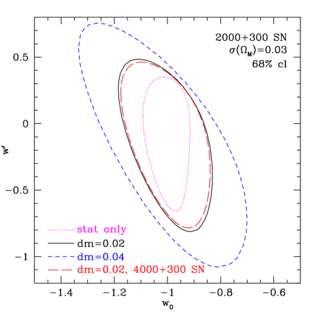
Figure 1: Dark energy parameter contours for three irreducible systematic cases. The central reference contour has only the intrinsic statistical error. Note the substantial increase in parameter error as the systematic is increased from $dm$ = 0.02 to 0.04. The two closely paired contours show that doubling the number of SNe will only increase parameter accuracy by $\approx$ 5$\%$.

To show the dominance of the systematic contribution over the statistical error we also double the number of supernovae in each bin (except the first bin representing the SNfactory sample). A fiducial input cosmology of $\Omega_{m}=0.3$, $w_{0}=-1.0$, $w^{\prime}=0$ is used along with a prior on $\Omega_{m}$ of 0.03. The intrinsic statistical error contours are also plotted for reference.

Let us note three important points about the systematic uncertainties evident from the figure: 1) they are the dominant source of error, 2) they impact parameter determination in nontrivial ways, and 3) allowing systematics to exceed 0.02 mag can strongly affect parameter estimation.

Overall one clearly sees that observing thousands more supernovae will not help in cosmological parameter estimation. Only by tighter bounds on the systematics can one improve precision. The systematics impose an error floor and become the dominant contribution over the statistical error for

$$N_{\rm bin}>(0.15/dm)^{2}.$$ (6)

For $dm=0.02$ mag this works out to about 55 supernovae per bin. It is worth noting some reasons, however, why one might want to exceed this number somewhat. These include:

1. Subsamples, e.g. collections of supernovae with similar spectral properties, allow carrying out a like-to-like comparison to identify and bound systematic uncertainties. Examination of supernovae within a bin, i.e. all at the same redshift, probes systematics while analyzing like subsamples at different redshifts probes cosmology more cleanly.

2. Lowering statistical errors well below the systematics floor reduces the total, quadratic sum error. For example twice as many supernovae as the break even number given by eq. (6) lowers the total error to within 22% of the floor.

3. Additional data can mitigate the effects of mis-estimation of the coherence scale, i.e. effective bin size, of the systematic. That is, since a systematic of 0.02 mag over a bin size of $\Delta z=0.05$ is roughly the same as $dm=0.014$ mag over $\Delta z=0.1$, more data ensures that statistical errors will not if the systematic error is smaller than 0.02 mag.

4. The complete supernova sample will include events that suffer significant host-galaxy dust absorption and gravitational demagnification. Beyond our systematic concerns, the light-curve and spectral measurements of these objects will carry reduced statistical weight due to their fainter appearance. An increased number of supernovae per redshift bin will make up for the expected range of data quality.

Overall, a contingency of roughly a factor of two more supernovae should prove satisfactory.

For the second point, Fig. 1 shows how a constant irreducible systematic of 0.02 magnitudes increases the parameter estimation errors. Note that the systematic does not simply scale up the contour but rather stretches it along the parameters’ correlation or degeneracy direction (very roughly defined by $w^{\prime}+4w_{0}$=const [Huterer & Turner 2001, Weller & Albrecht 2001, Linder & Huterer 2003]). Relative to the pure statistical error case, a 0.02 mag systematic increases the uncertainty in $w_{0}$ by a factor of 2 and $w_{1}$ by $26\%$. The effect of systematics on parameter estimation can also be a strong function of depth of the survey and underlying cosmological model, as discussed in the following sections.

Increasing the magnitude error beyond 0.02 mag, to 0.04, strongly degrades the precision with which the dark-energy parameters can be recovered. The constraint of $w_{0}$ suffers an additional 78% and $w^{\prime}$ incurs an extra 44% increase. Both of them become so imprecise that the limits are not useful. Therefore, bounding the systematics to 0.02 magnitudes is an important science goal for an experiment that hopes to detect the time variation of the dark-energy equation of state. Instruments and observation strategies must be specifically designed with this in mind. Garnering a sufficiently rich, well calibrated, and homogeneous set of data allows control for astrophysical and measurement effects so as to leave behind only a less than 0.02 mag residual.

Figure 2 illustrates the same systematics in the $w_{0}-\Omega_{M}$ plane.

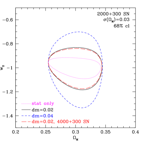
Figure 2: Contours for the mass density $\Omega_{M}$ versus the present dark energy equation of state $w_{0}$ for three irreducible systematics. As the systematic increases, the large increase in error for the equation of state is clearly apparent. The $\Omega_{M}$ parameter error stays constant since a prior constraint of $\sigma(\Omega_{M})$ = 0.03 dominates the estimation.

Again, the statistical errors are only a minor contribution to the total. Because the parameter estimation of $\Omega_{M}$ is dominated by the imposed prior $\sigma(\Omega_{M})=0.03$, the systematic acts in the $w_{0}$ direction. The uncertainty in $w_{0}$ increases over the purely statistical error by a factor of 2 and 4 when $dm$ = 0.02 and 0.04, respectively. Note that no prior assumption about $w^{\prime}$ was imposed, so the equation of state variable is $w_{0}$ not merely a constant $w$. Given that we are seeking to test the nature of dark energy, not assume it, and that there is no compelling theoretical model that predicts a constant value (other than possibly $-1$), we do not believe that results involving a constant $w$ serve any useful purpose for precision cosmology.

3.2 Random Irreducible Systematic – Linear in Redshift

Observations extending to the redshift depth necessary to probe dark energy, $z\mathrel{\mathchoice{\lower 3.6pt\vbox{\halign{$\mathsurround=0pt\displaystyle\hfil#\hfil$\cr>\crcr\sim\crcr}}}{\lower 3.6pt\vbox{\halign{$\mathsurround=0pt\textstyle\hfil#\hfil$\cr>\crcr\sim\crcr}}}{\lower 3.6pt\vbox{\halign{$\mathsurround=0pt\scriptstyle\hfil#\hfil$\cr>\crcr\sim\crcr}}}{\lower 3.6pt\vbox{\halign{$\mathsurround=0pt\scriptscriptstyle\hfil#\hfil$\cr>\crcr\sim\crcr}}}}1.5$, are challenging and one might well expect some possible errors to be exacerbated with increasing redshift. The restframe optical emission of supernovae shifts to the observer frame as $1+z$, with key spectral features at $z=1.7$ approaching 1.7 microns, so infrared capabilities are crucial to these high redshift observations. SNAP is specifically designed to include high-precision photometry out to 1.7 microns, but residual uncertainties enter. For example, models for Hubble Space Telescope (HST) spectrophotometric standards can disagree up to 1% at 1.7 microns [Bohlin 2002] due to the lack of precision exo-atmospheric, spectrophotometric measurements in the near infrared (NIR).

Since wavelength maps to redshift, larger errors in the infrared translate to increasing uncertainties at higher redshifts. To simulate the effect of such uncertainties on parameter determination, a linearly increasing systematic, $dm=\delta m\left(z/z_{max}\right)$, is adopted. As before, this is added in quadrature to the intrinsic 0.15 mag statistical error for supernova peak magnitudes in a binned approach:

$$\sigma_{m}=\sqrt{\frac{0.15^{2}}{N_{bin}}+\left(\delta m\frac{z}{z_{max}}\right)^{2}}.$$ (7)

Parameterization in terms of $z_{max}$ and $\delta m$ allows us to perform trade studies on other surveys with different redshift depths and infrared error limits. The SNAP design bounds the uncertainty for all relative photometric measurements to 0.02 mag, so the systematic ramps up as $dm=0.02(z/1.7)$.

Figure 3 shows parameter estimation confidence contours for some different survey depths and amplitudes of the linear systematic.

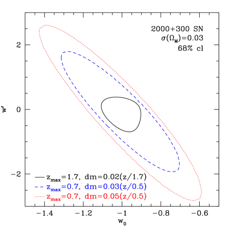
Figure 3: Dark-energy parameter contours with a linear systematic that increases with redshift. The SNAP contour includes a systematic of $dm=0.02(z/1.7)$ benefiting from the experiment’s high precision photometry and survey depth. Also plotted are two systematics simulating ground-based experiments that have larger photometric errors into the infrared and an effective redshift depth limited by the atmosphere.

These include SNAP, modeled as a space-based experiment with $z_{max}$ = 1.7 and $\delta m$ = 0.02 mag, and a ground-based experiment with an atmosphere-limited effective redshift of $z_{max}$ = 0.7 and either an optimistic $\delta m$ = 0.04 mag (corresponding to the line with $dm=0.03*(z/0.5)$ in Fig. 3) or a less challenging 0.07 mag (corresponding to $dm=0.05*(z/0.5)$ in Fig. 3) . The surveys were otherwise identical, with the same number of supernovae (the SNAP distribution of Table 1 was cut at $z_{max}$ and rescaled to total 2000 supernovae) and prior on the matter density.

The figure dramatically demonstrates that a deeper survey in redshift with the infrared capabilities to control systematics (especially dust extinction), opened up by the move to space, provides a superior lever arm in determining the cosmological parameters. Ground-based surveys, however, are limited for obtaining a homogeneous, complete data set to $z_{max}\mathrel{\mathchoice{\lower 3.6pt\vbox{\halign{$\mathsurround=0pt\displaystyle\hfil#\hfil$\cr<\crcr\sim\crcr}}}{\lower 3.6pt\vbox{\halign{$\mathsurround=0pt\textstyle\hfil#\hfil$\cr<\crcr\sim\crcr}}}{\lower 3.6pt\vbox{\halign{$\mathsurround=0pt\scriptstyle\hfil#\hfil$\cr<\crcr\sim\crcr}}}{\lower 3.6pt\vbox{\halign{$\mathsurround=0pt\scriptscriptstyle\hfil#\hfil$\cr<\crcr\sim\crcr}}}}0.7$ (see §6); increased statistics, such as provided here with 2000 supernovae, will not help. Figure 3 shows that even in the optimistic ground-based case, the parameter uncertainty increases by a factor of 3 in $w_{0}$ and a factor of 4 in $w_{1}$. The other case, $\delta m=0.05$, perhaps more realistically simulates the increase in uncertainties due to atmospheric absorption and night sky emission as one ventures into the infrared from the ground. Here the parameter estimation degrades by 24% in $w_{0}$ and 36% in $w_{1}$, just relative to the optimistic ground-based survey.

The equivalent blowing up of the confidence contours in the $w_{0}-\Omega_{M}$ plane is shown in Fig. 4.

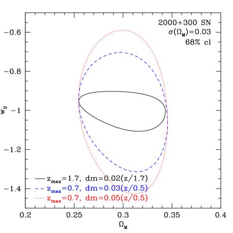
Figure 4: Error contours in the $\Omega_{M}-w_{0}$ plane for systematic errors linearly increasing with redshift. The SNAP measurement of $w_{0}$ shows the advantage of a deeper space-based survey with better photometric accuracy. There is a negligible change in the $\Omega_{M}$ measurement since the parameter is bounded by prior information.

Clearly, redshift depth and dedicated instrument design to bound systematic uncertainties are crucial to achieving precision cosmological parameter determination.

While the two models for systematics discussed in the last two subsections are not exhaustive, they do give a broad feel for different, physically motivated behaviors. These analyses indicate that the survey requirement of bounding systematics below 0.02 mag is both necessary and sufficient for the science goals of constraining the dark energy equation of state and its possible variation.

4 Systematic Biases

The other category of systematic effects considered is a coherent shift in magnitude for all supernovae at a given redshift. This could arise from broad astrophysical or detector issues such as residual uncertainties in intergalactic absorption, or selection effects such as Malmquist bias (see §6).

The effect of an offset in magnitude is a bias in the best fit parameters. That is, the data no longer guide the observer to the true underlying cosmology but rather to a false model. Obviously this is of great concern since we seek not only precise but accurate answers. Interestingly, the bias can actually somewhat reduce the dispersion around the best (incorrect) fit, since as mentioned in §2.3 the errors depend on the location within the parameter space. Thus one could be put into the situation of finding a wrong answer very precisely.

Bounding offsets below 0.02 mag, however, ensures that bias of the fit parameter from the true value is negligible, i.e. less than half the random, dispersive error. Furthermore, one is fortunate in that it is not the entire amplitude of the offset that alters the cosmological parameters of interest, but rather only its variation from the mean over the survey depth. Thus a constant offset has no effect on the cosmological and dark energy parameter estimation, and a linear increase to 0.02 mag at the maximum redshift is equivalent to a $-0.01$ mag shift at low redshift and a $+0.01$ mag shift at high redshifts. This point is sufficiently important that we present a formal proof in the Appendix.

4.1 Monte Carlo Analysis of Systematic Magnitude Offsets

Upon adding a constant 0.02 mag offset to all supernova magnitudes we verified by Monte Carlo that the best fit value of $\mathcal{M}$ was biased from an input of 0 to 0.02 while the fits for the cosmological parameters returned the true values and had errors indistinguishable from the case without such a systematic bias.

To investigate bias in the parameters and its amplitude relative to its random error, we introduced a magnitude offset that linearly increases with redshift. Specifically, we adopt $dm=\pm 0.03(z/1.7)$. Figure 5 shows the results for two different underlying cosmologies.

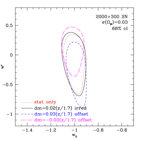
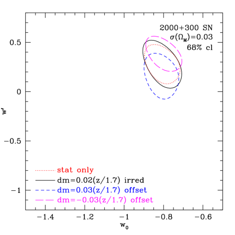
Figure 5: Dark-energy parameter contours after a magnitude bias is introduced. The solid lines include systematic errors but no offset, while the dashed curves have an offset but no systematic uncertainties. The upper plot corresponds to the fiducial universe with $w_{0}=-1$ and $w_{1}=0$, while the lower plot corresponds to the SUGRA-inspired scenario [Brax & Martin 1999, Weller & Albrecht 2001] with $w_{0}=-0.8$ and $w_{1}=0.3$. Note the large dependence of the precision attainable on the underlying cosmology.

The upper plot has an input model where the dark energy is a cosmological constant: $w_{0}=-1$, $w_{1}=0$, while the lower plot illustrates a model with time-varying equation of state for the dark energy: $w_{0}=-0.8$, $w_{1}=0.3$, corresponding to a supergravity inspired model [Brax & Martin 1999, Weller & Albrecht 2001].

In each case the dotted contours give the parameter estimation assuming only statistical errors on the SNAP supernovae. One can clearly see the dependence of errors and correlations on the location in parameter space, as discussed in §2.3. The effect of a random irreducible error, such as from §3.2, is to stretch the confidence contours, generally unequally for the two parameters. Such an expansion, shown by the solid contours, gives the increase in dispersion due to the extra random uncertainty.

However the effect of a coherent offset in magnitude, shown by the dashed contours, is very different. Here the contours are shifted in the $w_{0}-w_{1}$ plane in the presence of the bias, with the positive magnitude bias shifting the contours negatively in $w_{1}$. Little bias is seen in the $w_{0}$ direction because the supernova magnitude offset is highly correlated with the time variation $w_{1}$ and not so much with the single, present value of the equation of state. This can be seen as follows: Increasing the magnitude is dimming the supernovae; this means they have a greater luminosity distance at a given redshift than allowed by the fiducial cosmology, corresponding to more expansion of the universe and hence a more potent acceleration, provided by a more negative equation of state. Because the magnitude offset is here increasing with redshift, one requires a time varying change in the equation of state, i.e. a more pronounced $w_{1}$. (Recall a magnitude offset that is constant with redshift can be absorbed wholly into the ${\cal M}$ parameter, while a different $w_{0}$ does not lead to a monotonic magnitude offset.)

Also note that the biased confidence contours alter their shape and size slightly with respect to the unbiased, purely statistical error case. As discussed in §2.3, this is the result of the different location, and hence sensitivity, in parameter space. In fact, the linear bias may even decrease the statistical uncertainty. But roughly one can consider the effect of an offset magnitude systematic as shifting the statistical error contour to a biased best-fit value in the parameter space.

To guard against biased parameter determination one needs to bound systematic effects that give rise to redshift dependent magnitude offsets. In general, improved accounting for systematics by extending observations to high redshift and into the infrared, requiring a space based instrument, constrains such errors. Taking this into account, we consider linearly rising offsets reaching 0.02 and 0.04 mag at $z_{maz}=1.7$, and 0.04 and 0.07 at $z_{max}=0.7$. The first one represents the SNAP systematics goal and 0.04 mag illustrates the efects of failing to achieve it. The second two, ground, offsets are larger in magnitude to simulate the inherent difficulties in precision measurements through the atmosphere of higher redshift supernovae whose emission is shifted into the near infrared. The corresponding supernova distribution is taken to extend out to $z_{max}=0.7$ where ground based surveys run into degraded light curves and Malmquist bias due to the atmospheric limitations. The size of the ground offsets are chosen to give residual uncertainties slightly better and worse than proposed for the Essence supernova survey [Essence 2003].

As discussed before, the strongest effect is on the time variation of the equation of state, $w_{1}$. The four cases respectively give biases of $0.37\sigma$, $0.67\sigma$, $0.75\sigma$, $1.2\sigma$, where $\sigma$ is the corresponding statistical error for each case. How much bias is acceptable is somewhat subjective. If we require that the bias should not exceed $0.5\sigma$, then we see that even the ambitious ground-based survey fails this for $w_{1}$, and we cannot tolerate 0.04 mag offset for the deep, space-based survey. But a random irreducible systematic of these same amplitudes is far more damaging to parameter estimation than the coherent offsets discussed in this section. As mentioned in §§3.1,3.2, the depth and wavelength coverage accessible to a space-based survey substantially immunizes it against such uncertainties. For example the estimation of $w_{1}$ degrades by a factor of four when $z_{max}=0.7$ but only by 6% when $z_{max}=1.7$.

4.2 Low-Redshift Supernova Calibration Offset

A discontinuity in calibration between the proper SNAP sample and the low redshift Nearby Supernova Factory (SNF) measurements would present a different type of offset error. The SNF data play a critical role in reducing the uncertainty on ${\cal M}$, and hence $w^{\prime}$ through the correlation of these parameters. Since we conjoin datasets from two separate projects it behooves us to investigate a magnitude offset caused by differences in the observing methods and equipment.

To simulate such an effect we introduce a constant offset to all SNF supernovae relative to the SNAP dataset. Because the offset is at a single, low redshift, the major effect is on $w_{0}$. For an offset in the range 0.01–0.05 mag, the bias in fitting the $w_{0}$ parameter amounts to a fraction $1.2(dm/0.02)$ of the statistical error. So to keep the bias less than the statistical error, the offset should be restricted below 0.02 mag. Experimentally, spectrophotometric observations of the same standard stars by both SNF and SNAP should limit the offset below 0.01 mag. We have found that the biases in the other parameters, $\Omega_{m}$ and $w^{\prime}$, are indeed much smaller as a fraction of their statistical errors.

5 Calibration Uncertainty

The calibration procedure for a survey is an important potential source of systematic uncertainties. Since calibration enters so early in the data pipeline, these uncertainties can propagate through several stages. For instance, consider a calibration uncertainty on the blackbody temperatures, and hence fluxes, of two or more calibration sources and their correlations. That error would affect the measured fluxes of supernovae directly, as well as indirectly through the K-correction and the extinction corrections. The subsequent magnitude errors then affect the cosmological parameter determination.

Due to the complexity of the problem, we go beyond our previous analytic models and develop a complete Monte Carlo simulation. The central ingredient is a calibration model (like the two blackbody model just mentioned) with a certain number of free parameters (in this case, the temperatures of the blackbodies), their uncertainties, and the correlations among them. Realizations of calibration parameters are fed to a simulation of a SNAP-like mission. This includes statistical observational errors, multiband measurements, and the appropriate treatment of reddening and K-corrections. The result of each pass of the simulation is a set of SNe with their measured magnitudes and errors; many realizations then provide the individual supernova magnitude errors and correlations. The cosmology fitter uses this error covariance matrix to generate uncertainties and covariance contours in the cosmological parameters.

5.1 The Monte Carlo Simulation

In the Monte Carlo simulation, the supernova redshift distribution and cosmological model are as given in §2. As before, only the component of the calibration error which varies with redshift or, equivalently, with wavelength, matters for cosmological parameter estimation.

Differential dimming of the supernova magnitudes in the various observed wavelengths by dust is simulated using the standard parameterization of Cardelli, Clayton and Mathis [Cardelli, Clayton & Mathis 1989]. Values for the extinction value, $A_{V}$, come from a distribution obtained from a Monte Carlo simulation [Commins 2002] that places SNe in random positions of a galaxy with random orientation with respect to the line of sight. Values for the global extinction coefficient, $R_{V}$, are drawn from a Gaussian distribution centered at 3.1 and with standard deviation 0.3.

Once a set of parameters defining the calibration is chosen, it is used to compute zero points for each filter, which in turn enter the cross-filter K-corrections [Kim, Goobar & Perlmutter 1996]. The standard SNAP filter set has been simulated, although simplified to square filters. These involve nine filters logarithmically spaced and broadened in $1+z$ [Akerlof et al. 2003]. For each SN there is significant data in a minimum of three and a maximum of nine filters, depending on redshift. The flux in each filter is further smeared with an uncorrelated 2% error to account for statistical errors.

All optical and near-IR (in the SN frame) photometric data for a given SN are used to fit for two parameters: its magnitude and its extinction parameter $A_{V}$. By contrast, $R_{V}$ is assumed in the fit to be constant at 3.1. It has been found that this assumption introduces only a small bias in $w^{\prime}$ in the final result without affecting the result for $w_{0}$. As an example, sampling $R_{V}$ from a Gaussian distribution centered at 3.5 and with standard deviation 0.3 in the generation stage, while keeping $R_{V}$ fixed at 3.1 in the fitting stage, results in biases of $-0.15$ in $w^{\prime}$ and $-0.002$ in $w_{0}$.

After many realizations of the calibration parameters, enough statistics are collected to determine the central value and variance of the magnitude of each SN, as well as the correlations among them. These are input to the cosmology fit, along with an error of 0.15 magnitude added in quadrature to each supernova. This accounts for the statistical errors and the natural dispersion of the SN intrinsic magnitude. As previously, a flat $\Omega_{m}=0.3$ plus cosmological constant universe is fiducial, along with a Gaussian prior of 0.03 on $\Omega_{m}$.

5.2 Calibration Models

Two calibration models have been studied, broadly describing the classes of calibration procedures. In the first one [Lampton 2002], a single calibration source is taken as reference for all wavelengths, in the optical and infrared (IR) regions. The source is parameterized as a blackbody with a temperature $T$, known with a precision $\Delta T$. This model can be thought of as representing a hot white dwarf whose spectrum is well understood in both the optical and IR regimes. Typical values for $T$ would be around 20000 K, with uncertainties in the few percent range.

In a second, possibly more realistic, model [Deustua 2002], two calibrators are employed: one with temperature $T_{1}\pm\Delta T_{1}$ for the optical region, $\lambda\leq 1\mu{\mathrm{m}}$, and another with $T_{2}\pm\Delta T_{2}$ for the infrared region, $1\mu{\mathrm{m}}<\lambda<1.7\mu{\mathrm{m}}$. The errors in the two temperatures are taken to be correlated with correlation coefficient $\rho$. The optical calibration could be from a hot white dwarf, while the near infrared calibration could correspond to a NIST standard or a solar equivalent. In both cases, $T_{2}$ would be a few thousand Kelvin. The errors would again be a few percent. Although the two calibration sources are not expected to be correlated in themselves, correlations can enter either from common instrumental systems and data reduction or from the process of connecting the optical and near-IR calibrations.

5.3 Results

For the one-temperature model, Fig. 6 shows the 68% confidence level contours in the $w_{0}$-$w^{\prime}$ plane for the case without calibration errors, with a 1% error in $T$, and with a 10% error in $T$. Even allowing for a 10% uncertainty in $T$ results in a very small systematic error in the cosmological parameters. This unintuitive result can be explained by noting that in the Rayleigh-Jeans region a miscalibrated temperature corresponds mostly to a change in overall flux scale, which is absorbed in ${\cal M}$, and then the tilt, or color in astronomical terms, is treated by the extinction correction for flux differences between wavelengths. For a model with a single free parameter, $T$, the correction is almost perfect.

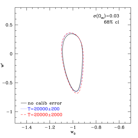
Figure 6: Joint probability contours for the determination of $w_{0}$ and $w^{\prime}$ without calibration error and with two values of the calibration error in the one-temperature model. The increase in uncertainty is quite small due to the use of multiple filters that correct for calibration variations between them in the same way as for extinction caused by dust.

Figure 7 shows the equivalent contours for the two-temperature model. Now the effect of the calibration error can be clearly seen. For 3% uncertainties it leads to an increase in the errors of $w_{0}$ and $w^{\prime}$ of around 20%, relative to the purely statistical errors.

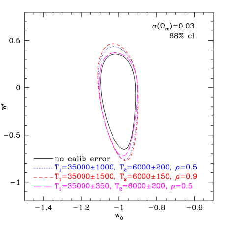
Figure 7: Joint probability contours for the determination of $w_{0}$ and $w^{\prime}$ without calibration error and with several values of the calibration errors and correlation in the two-temperature model. Calibration precision of order 3% in temperature is sufficient at these temperatures to keep parameter uncertainties within reasonable bounds.

The results are fairly insensitive to the correlation coefficient $\rho$ until it is nearly one. Then the calibration reduces to the one-temperature model. A 50% increase in the magnitude of the error in the optical region also does not strongly affect the parameter estimation. So long as the two-temperature model realistically approximates the entire calibration procedure, a moderate precision at the few percent level should suffice for calibration to pose only a minor contribution to uncertainty in the cosmological parameter estimation. In particular, 3% errors in both temperatures and any degree of correlation between the optical and infrared calibration measurements limit the increase in the overall error to $\mathrel{\mathchoice{\lower 3.6pt\vbox{\halign{$\mathsurround=0pt\displaystyle\hfil#\hfil$\cr<\crcr\sim\crcr}}}{\lower 3.6pt\vbox{\halign{$\mathsurround=0pt\textstyle\hfil#\hfil$\cr<\crcr\sim\crcr}}}{\lower 3.6pt\vbox{\halign{$\mathsurround=0pt\scriptstyle\hfil#\hfil$\cr<\crcr\sim\crcr}}}{\lower 3.6pt\vbox{\halign{$\mathsurround=0pt\scriptscriptstyle\hfil#\hfil$\cr<\crcr\sim\crcr}}}}20\%$ of the result without any calibration error.

Also note that if an optical calibration source can be determined to 1% (as the solar effective temperature already is [Deustua 2002]), then the error increase due to the calibration systematic uncertainty drops below 10%. And if improvements in observations and modeling allow a single body like a hot white dwarf to be used to calibrate the whole spectrum, then the precision of the calibration can be relaxed to 10%.

6 Malmquist Bias

Magnitude-limited searches for supernovae produce data samples with a selection effect called Malmquist bias: intrinsically brighter supernovae will be preferentially discovered. As supernovae at the fainter end of the luminosity function fall below the detection threshold, the mean intrinsic peak magnitude of discovered supernovae is biased lower (i.e. more luminous) than the mean for the whole population. The bias increases at higher redshifts as the apparent magnitudes of the supernova population grow fainter. This redshift-varying bias will thus enter the estimation of the cosmological parameters.

Measurements of the intrinsic dispersion in SNe Ia range from 0.25 – 0.35 magnitudes. However, correcting supernova magnitudes based on their light-curve time-evolution (stretch) can reduce the residuals to an rms of $\sim 0.10--0.15$ magnitudes. Note that this also leads to a selection effect: supernovae with high stretch are more likely to be found – they remain visible in the sky longer and are intrinsically brighter. However, a well-designed survey ensures that the stretch determination of discovered supernovae is unbiased. Here we consider Malmquist bias in the stretch-corrected luminosity function.

In principle, this error can be corrected for if the detection efficiency and intrinsic luminosity function are known. But the luminosity function should vary with the star formation history of the universe. Malmquist bias can thus stem from subtle systematic magnitude shifts arising from uncorrected population evolution of the progenitor systems. A precise bias correction requires well determined luminosity functions over the redshift span of interest. One way around this is by brute force: the detection threshold can be set much fainter than supernovae at the highest targeted redshift.

To illustrate the effect of Malmquist bias, we simulate light curves generated by a space survey with a SNAP-class telescope and a ground survey with a DMT-class (6.5m, e.g. LSST [LSST 2003]) telescope (augmenting the imager with an additional near infrared camera) sited at Mauna Kea. Ground observations are taken in the fiducial SNAP filter set with eight-hour observations. The observing cadence is four observer-frame days. Mauna Kea weather condition statistics are from [Sarazin 2002] and the seeing distribution compiled at Subaru is used [Aldering 2002]. We include host-galaxy extinction with an absorption distribution based on [Hatano, Branch & Deaton 1998].

We consider four simple detection triggers. The first two mimic triggers used in current ground searches and demand at least two points with signal-to-noise $S/N>5$ (7) in a single passband. The second two triggers require significant signal, $S/N>5$ (7), for two points in two passbands. This is important for the use of color time-evolution to distinguish SNe Ia from other transients. We require discovery before maximum light to allow spectral observations at peak brightness. The detection efficiencies for these triggers are shown in Fig. 8. The space mission discovers supernovae with almost perfect efficiency. The ground search suffers a fundamental level of inefficiency which is independent of intrinsic supernova luminosities since it is due to lost nights from poor weather. Efficiency from the ground suffers a further drop-off at redshifts $z>0.9-1.2$, depending on the trigger.

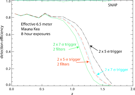
Figure 8: The efficiencies for detection of supernovae before maximum light for a SNAP-class space survey and an effective 6.5 meter telescope at Mauna Kea taking 8 hour exposures with a 4-day cadence. Only supernovae with host-extinction $A_{V}<0.5$ are included in the sample. The 0.85 ground efficiency at low redshift is predominantly due to lost nights due to weather. The slightly jagged nature of the curves is due to the finite number of supernova realized in the simulation.

The Malmquist biases induced by these triggers in space and ground missions are shown in magnitudes in Fig. 9. Depending on the exact form of the trigger, the Malmquist bias on the ground grows beginning at $z=0.9-1.3$. The more rigorous triggers with higher signal-to-noise thresholds or requiring detection in two bands have shallower redshift reach. From space, the bias remains $<0.01$ mag for all triggers over the full redshift range.

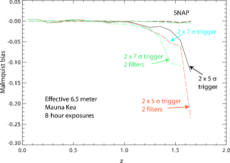
Figure 9: Malmquist bias for the four triggers for the space and ground-based surveys. Depending on the exact form of the trigger, the ground detection thresholds drop beginning at $0.9<z<1.3$. The space mission shows negligible Malmquist bias over the redshift range of interest. The small fluctuations are due to the finite number of supernovae used in calculating the detection efficiency.

We calculate the effect of this Malmquist bias on the ground searches described in §2.2. As a representative example, we consider the results from a trigger consisting of two $S/N>7$ points in a single filter. To illustrate the bias that occurs, we calculate the statistical errors and bias in the fit parameters assuming no irreducible systematic error for three ground surveys with $z_{max}=0.7,1.0$, and 1.3. For the two shallower surveys, the level of Malmquist bias is very low (cf. Fig. 9) and produces a bias that is small compared to the statistical errors. For the deepest survey, there is a significant 0.04 magnitude bias at $z_{max}=1.3$ that propagates into a significant component of the error budget; the bias in the measured cosmological parameters is now comparable to the pure statistical errors. There is little point in obtaining better statistics when the systematic errors dominate. Unless Malmquist bias can otherwise be eliminated or corrected for, deeper ground searches are thus fundamentally limited.

Note that this analysis only addressed the issue of Malmquist bias; there are difficulties posed to ground-based surveys by incompletely sampled lightcurves, lack of extinction measurements as the supernova flux redshifts into the infrared, atmospheric emission, etc.

7 Gravitational Lensing

Another effect on the measured flux of a supernova involves magnification or (more frequently) demagnification by weak gravitational lensing from intervening mass distributions. Since this conserves flux, the mean effect on supernovae at any redshift is null. However, the finite number of supernovae per redshift bin does not sample the entire magnification distribution, leading to a slight bias in the results from the Hubble diagram analysis. But this small bias can be determined from the data themselves [Amanullah, Mörtsell & Goobar 2003], independently of any model of gravitational lensing, and hence corrected, leaving only an additional systematic uncertainty coming from the limited statistical precision of the correction itself.

For weak lensing caused by large-scale structure, the rms of the shift is only a few percent and the mean shift can be averaged below 1% with only a couple dozen supernovae per redshift bin [Dalal et al. 2003, Holz & Linder 2003]. Here we consider the remaining case of lensing by compact objects, which generally gives a broader distribution of magnifications, following the method of [Amanullah, Mörtsell & Goobar 2003]. They show that the distribution of the biases in magnitude can be adequately parameterized by a functional form with three free parameters:

$$f(m) = \exp{\left(-\frac{\left(m-m_{0}\right)^{2}}{2\sigma^{2}}\right)}\ ,\ \ \ m\geq m_{c}$$

$$f(m) = \exp{\left(-\frac{\left(m-m_{0}\right)^{2}}{2\sigma^{2}}\right)}$$ (8)

$$+ b\cdot|m-m_{c}|\cdot 10^{s\cdot m}\ ,\ \ \ m\leq m_{c}\ ,$$

where $m$ is the bias after lensing, and the distribution takes into account the intrinsic dispersion of supernova magnitudes. The distribution represents a Gaussian with an extra tail toward demagnification. The constants $s$ and $m_{c}$ are set to 2.5 and 0 respectively. The three free parameters, $m_{0}$, $\sigma$ and $b$, will in general depend on the redshift and the assumed fraction of intervening mass in compact objects, $f_{p}$. We take $f_{p}=0.2$, which should give an upper bound on any plausible effect.

For a given redshift $z$ one can determine [Mörtsell 2002] the set $(m_{0},\sigma,b)$ that parameterizes the $m$ distribution . We then generate a Monte Carlo sample of $N(z)$ supernovae with the distorted $m$ distribution. This distribution can be measured in real data by shifting the magnitudes of all supernovae in the bin to the value they would have had if their redshift had been that of the center of the bin. For this, one has to assume a certain cosmology, but the result is fairly insensitive to this for reasonable bin widths, and by iterating the procedure after the cosmology fit all such dependency can be suppressed.

Once the $m$ distribution (in real data or through Monte Carlo) is obtained, a fit is made in order to measure the parameters of the distribution. Call the result $(m_{0}^{\prime},\sigma^{\prime},b^{\prime})$. Each parameter will have been measured with a certain error. The central value of the distribution corresponds to the net bias in magnitude that has to be corrected. Monte Carlo is used in order to compute the uncertainty in this central value as a function of the uncertainties in $(m_{0}^{\prime},\sigma^{\prime},b^{\prime})$. This procedure has been implemented for $z=0.5,1.0,1.5$ and $N(z)$ from the fiducial distribution in Table 1. The uncertainties after the corrections have been found to be 0.017, 0.018 and 0.021 mag for the three redshifts, therefore in line with the assumptions made in previous sections of a systematic error around 2%. A more realistic compact object fraction, $f_{p}<0.1$, would give a significantly smaller effect.

8 Evolution

In the previous sections we have addressed systematic uncertainties arising from the detectors, the observation strategy, and the light propagation. A potentially serious systematic error lies in the supernovae themselves. While supernovae have no direct influence from the cosmic time, i.e. they don’t “know” what redshift they are at [Branch et al. 2001], more subtle “evolutionary” effects can enter in the form of population drift.

For example, suppose the metallicity of a supernova had an influence on its absolute luminosity and supernovae at higher redshifts systematically had a lower metallicity than nearby supernovae. In this case, if the survey did not recognize and correct for this trend then the resulting Hubble diagram would be biased and the parameters resulting from the cosmology fit inaccurate.

Two approaches to this problem can be considered. Both require the survey to acquire and use the wealth of observational information that each supernova provides in the form of its time series of flux and its energy spectrum. Then the key assumption is that the state of the supernova is adequately described by these detailed measurements, that supernovae with the same lightcurve and spectrum indeed have the same absolute magnitude, that there are no “hidden variables”.

One approach is to carry out comprehensive modeling of Type Ia supernova explosions and radiation transport, examining numerically the effects of varying progenitor characteristics. The underlying physics proves remarkably robust and the final state possesses an extraordinary degree of “stellar amnesia” to the initial conditions [Höflich et al. 2003]. The remaining small variations in the light curves and spectra may even provide a tightening of the standard candle nature through a secondary correction parameter beyond stretch.

However we adopt only the purely empirical path of examining detailed observations of a wide range of supernovae. Any modeling is used solely to suggest features that might be of interest in the lightcurve and spectrum, and to serve as a subsidiary crosscheck. The Nearby Supernova Factory project [Aldering et al. 2002] will provide invaluable information on identifying secondary characteristics influencing the magnitude. Such a survey samples the breadth of galactic environments and physical conditions present at any redshift, e.g. the range of metallicities. However as mentioned above, there could be a population drift –a change in the proportion of environments at the different redshifts.

While analyses of supernovae with an average redshift of $z\approx 0.5$ [Sullivan et al. 2002] show no sign of a systematic trend (within the current precision) with galaxy type or location of the supernova within the galaxy, we need to guard against the possibility at higher redshift. This leads to the program of “like-to-like” comparisons [Perlmutter & Schmidt 2003, Branch et al. 2001]. One categorizes the supernovae based on the detailed observations into subsamples with similar intrinsic characteristics, e.g. ratios of peak-to-late-time light-curve magnitude, ultraviolet properties, line ratios, etc. Then these narrow subclasses are compared across different redshifts, taking that like spectral and flux characteristics imply like intrinsic magnitudes –with sufficiently comprehensive measurements there is nowhere for a change to hide. This procedure, we emphasize, is purely empirical and does not depend on any theoretical model of the luminosity or of evolution. The mantra is that like supernovae at different redshifts give a clear view of cosmology, and different supernovae at like redshifts alert us to intrinsic systematics.

To test this approach, we divided the total sample of SNe in up to ten subsamples, each with roughly the same number of SNe and similar distribution in $z$, allowing a different intrinsic magnitude (i.e. ${\cal M}$) for each subsample in the fit. The fit returned the same cosmological parameters as the fit with just one ${\cal M}$, with a negligible increase in their statistical error.

We then allow the subsamples to have different redshift distributions, mocking up population drift. The 2000 supernovae are divided into three subsamples of roughly the same size, one of them with the number of supernovae rising linearly with $z$, another one decreasing linearly and the third one flat, so that the total sample is uniform in redshift. When a different value for the intrinsic magnitude is allowed for each subsample, one finds a small (less than 4%) increase in the uncertainty in $w_{0}$, relative to the case of a single sample of 2000 SNe uniformly distributed in $z$ and with a single intrinsic magnitude for all the SNe. An even smaller increase (below 2%) is seen for $w^{\prime}$, while essentially no change is observed for $\Omega_{m}$. Thus comprehensive data collection, including spectra, together with like vs. like analysis, appear to provide a robust solution for potential evolutionary systematics.

9 Conclusion

Precision cosmological observations offer the hope to uncover essential properties of our universe, including the nature of the dark energy that causes the present accelerating expansion and could determine its fate. But hand in hand with these advances must go understanding of the systematic effects that could mislead us. We have presented in some generality as well as some detail several possible sources of systematic uncertainty for the Type Ia supernova method of mapping the cosmological distance-redshift relation.

In every case we have shown that the residual uncertainties after using detailed measurements of the light curves and spectra, when bounded below 0.02 mag, do not significantly interfere with the goal of accurate estimation of the matter and dark energy densities, $\sigma(\Omega_{\Lambda})=0.03$, the dark energy equation of state today, $\sigma(w_{0})=0.07$, and a measure of its time variation, $\sigma(w^{\prime})=0.3$.

This supports with analytic, numerical, and Monte Carlo simulations the conclusion that a well designed satellite survey of about 2000 Type Ia supernova, observed out to redshift $z=1.7$, with complete lightcurve characterization and a spectrum for every supernova, can succeed in answering some of the most fundamental questions about our universe and physics.

No other cosmological probes, promising though they might appear, have yet addressed the crucial question of systematics with the same degree of rigor. When this is established they may well offer valuable complementarity. For the supernova method, we note that the combined optical and near infrared observations and redshift reach to $z=1.7$ are critical elements in reducing the impact of systematic uncertainties.

Appendix A Fisher Matrix Analysis of Systematic Magnitude Offsets

A constant level of magnitude offset can be absorbed wholly into the ${\cal M}$ parameter, leaving the cosmological parameters unaffected. We use the following proof as an illustration of the Fisher matrix method.

The Fisher, or information, matrix method of error estimation approximates the parameter likelihood surface by a paraboloid in the vicinity of its maximum. As long as the parameter errors are small, the Fisher method gives an excellent approximation to a full maximum likelihood analysis. The Fisher matrix relates the observables, in this case the set of supernova magnitudes $m(z)$, to the parameters $\theta=\{\Omega_{m},w_{0},w^{\prime},{\cal M}\}$ through the sensitivities $\partial m/\partial\theta$:

$$F_{ij}={1\over\sigma_{m}^{2}}\int dz\,N(z){\partial m\over\partial\theta_{i}}{\partial m\over\partial\theta_{j}}\,,$$ (9)

where $\sigma_{m}=0.15$ and $N(z)$ is the number of SNe in a redshift bin around $z$. The error, or covariance, matrix is the inverse of this, so for example $\sigma^{2}(w_{0})=(F^{-1})_{w_{0}w_{0}}$.

External or prior information is incorporated simply by adding the Fisher matrices. The simplest example is a Gaussian prior on a single parameter, say $\Omega_{m}$, which corresponds to adding an information matrix empty save for a single entry in the appropriate diagonal space; if prior information determines $\Omega_{m}$ to $\pm 0.03$ then the matrix entry is $1/(0.03)^{2}$. Rules of matrix algebra allow one to calculate how such a prior affects all the entries in the covariance matrix, i.e. the parameter estimation errors.

A systematic offset in the observed magnitude similarly propagates into the results, in the form of a bias giving a best fit parameter value different from the input cosmological model (because this shifts locations on the likelihood surface it will also have a small effect on the statistical part of the errors). Denoting the offset as $\delta m(z)$, matrix algebra provides the bias relation

$$\delta\theta_{i}=F^{-1}{}_{ij}{1\over\sigma_{m}^{2}}\int dz\,N(z)\,\delta m(z){\partial m\over\partial\theta_{j}}\,,$$ (10)

where summation over repeated indices is implied. This allows straightforward calculation of the induced bias, within the Fisher formalism. Note that this looks similar to the Fisher matrix expression (9) but only contains a single sensitivity factor.

However, the nuisance parameter ${\cal M}$ is purely additive and so has sensitivity $\partial m/\partial{\cal M}=1$. Thus $F_{{\cal M}\theta}$ has only one apparent derivative factor, like the bias expression. Indeed if we separate out the redshift independent part of the systematic, $\delta m(z)=\delta m_{0}+dm(z)$, then the term containing the constant offset reduces to

$$\delta\theta_{i}=F^{-1}{}_{ij}F_{j{\cal M}}\,\delta m_{0}=\delta m_{0}\,\delta_{i{\cal M}}.$$ (11)

So the constant part of the offset systematic only causes a bias in the nuisance parameter ${\cal M}$ and does not affect the cosmological parameters. One could choose this to represent the mean offset, or to remove a constant from the offset such that the magnitude systematic is defined to be zero at zero redshift.

References

- [Akerlof et al. 2003] Akerlof, C. et al., 2003, in preparation
- [Aldering 2002] Aldering, G., 2002, SNAP internal memo
-
[Aldering et al. 2002]
Aldering, G. et al., 2002, Proc of SPIE, 4836;
http://snfactory.lbl.gov/spie_2002.pdf - [Allen, Schmidt & Fabian, 2002] Allen, S.W., Schmidt, R.W., & Fabian, A.C., 2002, MNRAS, 334, L11 [arXiv:astro-ph/0205007]
- [Amanullah, Mörtsell & Goobar 2003] Amanullah, R., Mörtsell, E., & Goobar, A., 2003, A&A, 397, 819
- [Bohlin 2002] Bohlin, R., 2002, Proc. of 2002 HST Calibration Workshop, 97
- [Branch et al. 2001] Branch, D., Perlmutter, S., Baron, E., & Nugent, P., 2001, arXiv:astro-ph/0109070
- [Brax & Martin 1999] Brax, P. & Martin, J., 1999, PLB 468, 40
- [Cardelli, Clayton & Mathis 1989] Cardelli, J. A., Clayton, G. C., & Mathis, J. S., 1989, ApJ, 345, 245
-
[Carroll 2001]
Carroll, S. M., 2001, arXiv:astro-ph/0107571,
http://pancake.uchicago.edu/~carroll/preposterous.html - [Commins 2002] Commins, E. D., 2002, SNAP internal note
- [Dalal et al. 2003] Dalal, N., Holz, D. E., Chen, X., & Frieman, J. A., 2003, ApJL, 585, L11
- [Deustua 2002] Deustua, S. E., 2002, private communication
- [Essence 2003] Essence, 2003, http://www.ctio.noao.edu/essence
- [Frieman et al. 2003] Frieman, J. A., Huterer, D., Linder, E. V., & Turner, M. S., 2003, PRD, 67, 083505 [arXiv:astro-ph/0208100]
- [Hatano, Branch & Deaton 1998] Hatano, K., Branch, D., & Deaton, J., 1998, ApJ, 502, 177 [arXiv:astro-ph/9711311]
- [Höflich et al. 2003] Höflich, P., Gerardy, C., Linder, E. & Marion, H., 2003, arXiv:astro-ph/0301334, in “Stellar Candles”, eds. Gieren et at., Lecture Notes in Physics
- [Holz & Linder 2003] Holz, D. E. & Linder, E. V., 2003, in preparation
- [Huterer & Turner 2001] Huterer, D. & Turner, M. S., 2001, PRD, 64, 123527
- [Kim, Goobar & Perlmutter 1996] Kim, A., Goobar, A., & Perlmutter, S., 1996, PASP, 108, 190
- [Lampton 2002] Lampton, M. L., 2002, SNAP internal note
- [Linder & Huterer 2003] Linder, E. V. & Huterer, D., 2003, PRD, 67, 081303 [arxiv:astro-ph/0208138]
- [LSST 2003] LSST, 2003, http://www.dmtelescope.org
- [Minuit 2002] Minuit, 2002, http://wwwinfo.cern.ch/asdoc/minuit/minmain.html
- [Mörtsell 2002] Mörtsell, E., 2002, private communication. See also [Amanullah, Mörtsell & Goobar 2003]
- [NAG 2002] NAG, 2002, http://anaphe.web.cern.ch/anaphe/gemini.html
- [Oguri, Suto & Turner 2003] Oguri, M., Suto, Y., & Turner, E. L., 2003, ApJ, 583, 584 [arXiv:astro-ph/0210107]
- [Perlmutter & Schmidt 2003] Perlmutter, S. & Schmidt, B. P., 2003, arXiv:astro-ph/0303428, to appear in “Supernovae and Gamma Ray Bursts”, ed. K. Weiler, Lecture Notes in Physics
- [Perlmuter et al. 1999] Perlmutter, S. et al., 1999, ApJ, 517, 565
- [Phillips et al. 1999] Phillips, M. M. et al., 1999, AJ, 118, 1776 [arXiv:astro-ph/9907052]
- [Riess, Press & Kirshner 1996] Riess, A. G., Press, W. H., & Kirshner, R. P., 1996, ApJ, 473, 88 [arXiv:astro-ph/9604143]
- [Riess et al. 1998] Riess, A. G. et al., 1998, AJ, 116, 1009
- [Sarazin 2002] Sarazin, M., 2002, ESPAS Site Summary Series: Mauna Kea, ESO report
- [SNAP 2003] SNAP, 2003, http://snap.lbl.gov
- [Spergel et al. 2003] Spergel, D. N. et al., 2003, arXiv:astro-ph/0302209
- [Sullivan et al. 2002] Sullivan, M. et al., 2002, arXiv:astro-ph/0211444
- [Tripp & Branch 1999] Tripp, R. & Branch, D., 1999, Correction for Type Ia Supernovae,” ApJ, 525, 209 [arXiv:astro-ph/9904347]
- [Weller & Albrecht 2001] Weller, J. & Albrecht, A. , 2001, PRL, 86, 1939