On the Origin of Intracluster Entropy

Abstract

The entropy distribution of the intracluster medium and the shape of its confining potential well completely determine the X-ray properties of a relaxed cluster of galaxies, motivating us to explore the origin of intracluster entropy and to describe how it develops in terms of some simple models. We present an analytical model for smooth accretion, including both preheating and radiative cooling, that links a cluster’s entropy distribution to its mass accretion history and shows that smooth accretion overproduces the entropy observed in massive clusters by a factor $\sim 2$-3, depending on the mass accretion rate. Any inhomogeneity in the accreting gas reduces entropy production at the accretion shock; thus, smoothing of the gas accreting onto a cluster raises its entropy level. Because smooth accretion produces more entropy than hierarchical accretion, we suggest that some of the observed differences between clusters and groups may arise because preheating smooths the smaller-scale lumps of gas accreting onto groups more effectively than it smooths the larger-scale lumps accreting onto clusters. This effect may explain why entropy levels at the outskirts of groups are $\sim 2$-3 times larger than expected from self-similar scaling arguments. The details of how the density distribution of accreting gas affects the entropy distribution of a cluster are complex, and we suggest how to explore the relevant physics with numerical simulations.

1 Introduction

Not so very long ago, people who studied clusters of galaxies were often asked how the X-ray emitting gas gets so hot. The answer is simple, of course. If radiative cooling is negligible, then gravitationally driven processes will heat diffuse gas to the virial temperature of the potential well that confines it. A tougher question would have been to ask why the intracluster medium has the density that it does. In order to answer that question, one needs to know what produces the entropy of the X-ray emitting gas.

Entropy is of fundamental importance because a cluster’s intergalactic gas will convect until its isentropic surfaces coincide with the equipotential surfaces of the dark-matter potential. Thus, the entropy distribution of a cluster’s gas and the shape of the dark-matter potential well in which that gas sits completely determine the large-scale X-ray properties of a relaxed cluster of galaxies (see Voit et al. 2002 and references therein). The gas density profile $\rho(r)$ and temperature profile $T(r)$ in this state of convective and hydrostatic equilibrium are just manifestations of the underlying entropy distribution. If we wish to link these X-ray observables to the process of cluster formation, we therefore need to understand how the growth of cosmic structure generates intracluster entropy and how processes like radiative cooling and non-gravitational heating by supernovae and active galactic nuclei modify that entropy distribution.

One way to approach the problem of gravitationally driven entropy generation is through spherically symmetric numerical models of smooth accretion, in which gas passes through an accretion shock as it enters the cluster (e.g., Knight & Ponman 1997; Tozzi & Norman 2001). If the incoming gas is cold, then the accretion shock is the sole source of intracluster entropy. If instead the incoming gas has been heated before passing through the accretion shock, then the Mach number of the shock is smaller and the intracluster entropy reflects both the amount of preheating and the production of entropy at the accretion shock.

In reality, however, the accreting gas is lumpy, not smooth. Incoming gas associated with accreting subhalos enters the cluster with a wide range of densities. There is no well-defined accretion shock but rather a complex network of shocks as different lumps of infalling gas mix with the intracluster medium of the main halo. Yet, despite this complexity, numerical simulations of hierarchical structure formation show that the resulting entropy profile is similar to that found in the smooth accretion models (Borgani et al. 2001, 2002).

This paper outlines some simple analytical models designed to clarify the processes that determine the entropy of intracluster gas. As has become customary in this field, we will refer to

$$K\;=\;\frac{P}{\rho^{5/3}}\;=\;\frac{1}{\mu m_{p}}\left(\frac{n_{e}}{\rho}\right)^{2/3}\frac{T}{n_{e}^{2/3}}$$ (1)

as the “entropy” of the gas, while recognizing that the formal thermodynamic entropy per particle for a gas of non-interacting monatomic particles is

$$s=\ln K^{3/2}+s_{0}\;\;,$$ (2)

where $s_{0}$ depends only on fundamental constants and the mixture of particle masses. Because we express temperatures in energy units throughout the paper, Boltzmann’s constant is absorbed into $T$ and $s$ becomes a dimensionless quantity. The object of our investigation is to understand the origin of the intracluster entropy distribution $K(M_{g})$, defined so that the inverse function $M_{g}(K)$ is the mass of gas with entropy $<K$.

Section 2 computes the entropy distribution arising from smooth spherical accretion of cold gas. It presents a simple analytical formulation for smooth accretion relating the entropy distribution of a cluster directly to its mass accretion rate. The shape of the resulting entropy distribution is similar to that of simulated and observed clusters but its normalization is too large by a factor $\sim$2-3, indicating that inhomogeneities in the accreting gas must be taken into account. Because of this difference between smooth accretion and inhomogeneous accretion, the normalization of the intracluster entropy profile reflects the lumpiness of the gas that accreted onto the cluster.

Section 3 shows how preheating and radiative cooling change the entropy distribution produced by smooth accretion. We demonstrate that modest amounts of preheating raise the entropy distribution expected from cold accretion by an additive term proportional to the initial entropy of the incoming gas. However, large amounts of preheating, comparable to the characteristic entropy of the halo, suppress entropy production because they expand the intracluster medium and reduce the shock velocity at the accretion front. Including simple corrections for preheating and radiative cooling yields analytical smooth-accretion models whose entropy distributions agree well with the numerical models of Tozzi & Norman (2001). However, the effects of preheating on hierarchical accretion are qualitatively different because preheating smooths the gas accreting onto a cluster, potentially boosting its postshock entropy much more than the simple additive correction applied to smooth accretion.

Section 4 presents evidence suggesting that accretion of baryons onto groups was smoother than accretion onto clusters. We show that groups must have significant entropy gradients. Otherwise, the observed values of core entropy cannot be reconciled with the observed X-ray luminosity-temperature ($L$-$T$) relation. Polytropic models consistent with both the core entropy and the $L$-$T$ relation imply that entropy levels in the outer parts of groups are $\sim$2-3 times higher than expected from simulations without cooling or preheating and from self-similar scaling of clusters. These findings are consistent with existing observations of groups and suggest a transition from lumpy accretion to smooth accretion below a mass scale $\sim 10^{14}\,h^{-1}\,M_{\odot}$.

Section 5 explores how the lumpiness of accreting gas determines the intracluster entropy distribution. We present a naive calculation applying simple accretion shocks to discrete accreting subhalos and show that this simple picture fails to produce enough entropy. We then consider what adjustments to the preshock density and preshock velocity would be needed to produce the proper amount of entropy through simple accretion shocks. However, the situation could well be more complicated than this because dense accreting lumps do not necessarily thermalize all their incoming kinetic energy within the accreting gas. We therefore generalize the idea of an accretion shock and investigate entropy production by dissipation of turbulence and relatively weak shocks created as accreting subhalos circulate within the intracluster medium. Somehow the process of hierarchical accretion in the absence of preheating and radiative cooling produces self-similar entropy profiles in groups and clusters, and we assess the amount of heat input needed to preserve this self-similarity. If this heating mode is significant, then it can partially offset radiative cooling in the cores of clusters, and we suggest how to test for this effect using numerical simulations.

Section 6 summarizes our findings.

2 Smooth Accretion of Cold Gas

Let us first consider the case of cold accreting gas, in which the pressure of the incoming gas is negligible. We will assume a spherically symmetric geometry, so that mass accretes in a series of concentric shells, each with baryon fraction $f_{b}$, that initially comove with the Hubble flow. In this simple model, a shell that initially encloses total mass $M$ reaches zero velocity at the turnaround radius $r_{\rm ta}$ and falls back through an accretion shock at radius $r_{\rm ac}$. We will find that the entropy distribution in this case is determined primarily by the rate at which matter accretes onto the cluster and yields an entropy distribution between $K\propto M_{g}$ and $K\propto M_{g}^{4/3}$.

2.1 Postshock Entropy

Because the cold accreting gas is effectively pressureless, the equations that determine the postshock entropy are

$$\dot{M}_{g} = 4\pi r_{\rm ac}^{2}\rho_{1}v_{\rm ac}$$ (3)

$$v_{\rm ac}^{2} = \frac{2GM\xi}{r_{\rm ac}}$$ (4)

$$\xi = 1-\frac{r_{\rm ac}}{r_{\rm ta}}$$ (5)

$$T_{2} = \frac{1}{3}\mu m_{p}v_{\rm ac}^{2}$$ (6)

$$\rho_{2} = 4\rho_{1}\;\;,$$ (7)

where $\rho_{1}$ is the preshock gas density and $T_{2}$ and $\rho_{2}$ are postshock quantities. Equations (6) and (7) are restatements of the jump conditions for strong shocks, assuming that the postshock velocity is negligible in the cluster rest frame (e.g., Landau & Lifshitz 1959; Cavaliere, Menci, & Tozzi 1997), and equation (5) is strictly true only for cosmologies with $\Lambda=0$. The postshock entropy produced by smooth accretion of cold gas at time $t$ is then

$$K_{\rm sm} = \frac{v_{\rm ac}^{2}}{3(4\rho_{1})^{2/3}}$$ (8)

$$= \frac{1}{3}\left(\frac{4\pi G^{2}\xi^{2}}{f_{b}}\right)^{2/3}\left[\frac{d\ln M}{d\ln t}\right]^{-2/3}(Mt)^{2/3}\;\;,$$

where $f_{b}=0.02h^{-2}\Omega_{\rm M}^{-1}$ is the universal baryon fraction. Thus, the entropy profile arising from smooth accretion of cold gas depends entirely on the ratio $r_{\rm ac}/r_{\rm ta}$ and the accretion history $M(t)$.

2.2 Shock Radius

The ratio of the shock radius to the turnaround radius should remain nearly constant with time in the case of cold accretion. One standard approach to estimating the virial radius of a cluster is to assume that it is precisely equal to half the turnaround radius of the shell that is currently accreting. Setting the shock radius equal to the virial radius defined in this way implies $\xi=0.5$ by definition.

More generally, one can assume that the shock occurs at the radius $r_{\Delta}$ within which the mean density is $\Delta$ times the critical density $\rho_{\rm cr}$. In that case, $r_{\rm ac}=(2GM/H^{2}\Delta)^{1/3}$, where $H=H_{0}[\Omega_{\rm M}(1+z)^{3}+(1-\Omega_{\rm M})]^{1/2}$ in a flat cosmology. The corresponding turnaround radius can be found from the equation of motion

$$\ddot{r}=-\frac{GM}{r^{2}}+\frac{\Lambda r}{3}\;\;.$$ (9)

In the limit of a vanishingly small cosmological constant $\Lambda$, a bound shell obeys the familiar parametric solution $r=r_{\rm ta}[(1-\cos\theta_{M})/2]$, $t=t_{\rm vir}[(\theta_{M}-\sin\theta_{M})/2\pi]$, with $r_{\rm ta}=[(2GMt_{\rm vir}^{2})/\pi^{2}]^{1/3}$ for a shell that collapses to the origin at time $t_{\rm vir}$. The solution for $\Omega_{\Lambda}=\Lambda/3H_{0}^{2}=0.7$ is not much different because the $\Lambda$ term is always small. The quantity $\Lambda r/3$ is never greater than $0.14GM/r^{2}$ during the trajectory of any shell that has accreted by the present time, which is why we neglected any $\Lambda$-dependence in equation (5). The time to fall from $r_{\rm ac}\lesssim 0.5r_{\rm ta}$ to the origin is also negligible, so we obtain $r_{\rm ac}/r_{\rm ta}\approx(\pi^{2}/H^{2}t^{2}\Delta)^{1/3}$. In this paper, we will generally set $r_{\Delta}=r_{\rm ta}/2$, unless stated otherwise.

The self-similar solution of Bertschinger (1985) for cold accretion with $\Omega_{\rm M}=1$ and $f_{b}\ll 1$ provides some support for these assumptions. In that model, the radius of the accretion shock remains fixed at 0.347 times the radius of the shell that is currently turning around. Because $M\propto t^{2/3}$ in the Bertschinger solution and the shell turning around at time $t$ accretes at time $2t$, this model implies $\xi=1-0.347\cdot 2^{8/9}=0.36$.

In a self-consistent model of a shock-bounded intracluster medium, the ram pressure of infalling gas at the accretion shock must balance the thermal pressure at the outer boundary of the hydrostatic region (i.e., $P+\rho v^{2}$ must be continuous across the accretion shock.) Thus, the value of $\xi$ depends on both the accretion rate of the cluster and its internal structure. Appendix A develops self-consistent solutions for the equilibrium shock radius in the case of a polytropic equation of state and a time-varying accretion history. As long as the accreting gas is cold, we find that $\xi\approx 0.35-0.6$ for the accretion histories considered in this paper. However, preheating of the accreting gas can drive $\xi$ much lower, as we will discuss in § 3.2.

2.3 Accretion History

Because of the constancy of $\xi$, the entropy distribution for cold, smooth accretion directly reflects the accretion history $M(t)$. A rough estimate of $M(t)$ can be obtained from extended Press-Schechter theory (Bond et al. 1991; Bower 1991; Lacey & Cole 1993). If we restrict our attention to virialized halos that are much more massive than the characteristic mass, then $M\propto\omega^{-3/(n+3)}$, where $n$ is the power-law slope of the perturbation spectrum and $\omega\equiv\delta_{c}(t)D(t_{0})/D(t)$ is a function of the critical threshold for virialization $\delta_{c}(t)$ and the growth function $D(t)$ (e.g., Lacey & Cole 1993; Voit & Donahue 1998). In a flat cosmology with $\Omega_{\rm M}=0.3$ at $t_{0}$, the approximation $D(t)\propto t^{0.63}$ is accurate to within 6% from $0.01t_{0}$ to $t_{0}$. For the relevant range of power-spectrum indices ($-2\lesssim n\lesssim-1$), we therefore find $M\propto t^{\zeta}$, with $0.9\lesssim\zeta\lesssim 1.9$, yielding a power-law entropy distribution between $K_{\rm sm}\propto M_{g}$ and $K_{\rm sm}\propto M_{g}^{1.4}$. These simple relations agree well with those found by both spherically symmetric hydrodynamical calculations (Tozzi & Norman 2001) and three-dimensional simulations (Borgani et al. 2001, 2002). However, to do a proper comparision, we need a more accurate expression for $M(t)$.

Figure 1: Accretion histories for halos of total mass $M(t_{0})$ at the present time $t_{0}$. Filled squares give the logarithmic mean of the maximum progenitor mass $M_{\rm max}$ in the merger history of a halo of mass $M(t_{0})=10^{15}h^{-1}M_{\odot}$, computed from 1000 realizations of the Lacey & Cole (1993) algorithm. Open squares and filled triangles show the corresponding quantity for $M(t_{0})=10^{14}h^{-1}M_{\odot}$ and $10^{13}h^{-1}M_{\odot}$. Error bars indicate one standard deviation. The solid line shows the best fitting parabola in $\log M(t)$-$\log t$ space for $M(t_{0})=10^{15}h^{-1}M_{\odot}$. The long and short-dashed lines show best fits for $M(t_{0})=10^{14}h^{-1}M_{\odot}$ and $10^{13}h^{-1}M_{\odot}$, respectively. The dotted line indicates the accretion history used by Tozzi & Norman (2001) for their $10^{15}\,h^{-1}\,M_{\odot}$ cluster in a $\Lambda$CDM cosmology.

Figure 1 illustrates some useful expressions for $M(t)$ derived from the merger-tree algorithm of Lacey & Cole (1993) for a $\Lambda$CDM cosmology with $\Omega_{M}=0.3$, $\Omega_{\Lambda}=0.7$, and $\sigma_{8}=0.9$. We computed 1000 realizations of merger trees leading to a present day halo mass $M(t_{0})$, assumed that $M(t)$ was equal to the maximum progenitor halo mass $M_{\rm max}$ at time $t$, and determined the best-fitting parabola in $\log M$–$\log t$ space. The coefficients of those best fits are given in Figure 1. As expected, the effective value of $\zeta$ is in the range $1\lesssim\zeta\lesssim 2$, except for the lower-mass halos ($10^{13}h^{-1}M_{\odot}$) at late times. Figure 2 shows the logarithmic slope $d\ln K/d\ln M_{g}$ implied by these fits. Note that this slope generally remains between 1.0 and 1.3 but rises above that in the outer parts of lower-mass halos because of the diminishing accretion rate as $t$ approaches $t_{0}$.

The near linearity of the relation between $K$ and $M_{g}$ is what sets the effective polytropic index of intracluster gas outside the cluster core. Because the underlying potential is nearly isothermal, the gas density scales approximately as $\rho\propto r^{-2}$, implying $M_{g}\stackrel{{\scriptstyle\propto}}{{\sim}}\rho^{-1/2}$. Thus, the relation $K\propto M_{g}$ leads to $P\propto\rho^{\gamma_{\rm eff}}$ with $\gamma_{\rm eff}\approx 1.2$ and $K\propto M_{g}^{1.2}$ leads to $\gamma_{\rm eff}\approx 1.1$. Observations indicate that $\gamma_{\rm eff}\approx 1.1-1.2$ in hot clusters (Markevitch et al. 1998, 1999; Ettori & Fabian 1999; DeGrandi & Molendi 2002), supporting the idea that $K\stackrel{{\scriptstyle\propto}}{{\sim}}M_{g}$ when gravitationally-driven processes dominate the production of intracluster entropy.

Figure 2: Logarithmic slope $d\ln K/d\ln M_{g}$ of the entropy profile $K_{\rm sm}(M_{g})$. The profile for a $10^{15}\,h^{-1}\,M_{\odot}$ halo given by equation (2.1) is nearly linear, while the profiles for lower-mass halos steepen near the outskirts of the cluster. This steepening arises because of the diminishing accretion rate at late times.

2.4 Entropy Profile

We can now compare the entropy profile produced by smooth accretion of cold gas to entropy profiles computed in other ways. To simplify those comparisions, we will recast the entropy profiles in dimensionless form. Because the mean matter density within $r_{\Delta}$ is $\Delta\rho_{\rm cr}$, the characteristic temperature associated with overdensity $\Delta$ is $T_{\Delta}=GM_{\Delta}\mu m_{p}/2r_{\Delta}$, where $M_{\Delta}=4\pi r_{\Delta}^{3}\Delta\rho_{\rm cr}/3$. These definitions lead to a characteristic entropy in the baryons of $K_{\Delta}=T_{\Delta}/[\mu m_{p}(\Delta f_{b}\rho_{\rm cr})^{2/3}]$. In this section, we divide all profiles by the cosmology-independent entropy scale $K_{200}$ obtained by setting $\Delta=200$. The dimensionless entropy is then $\hat{K}\equiv K/K_{200}$, with $K_{200}=(3.3\times 10^{34}\,{\rm erg\,cm^{2}\,g^{-5/3}})(M_{200}/{10^{15}\,h^{-1}\,M_{\odot}})^{2/3}$ for $\Omega_{\rm M}=0.3$. In section 5 we will find it more useful to work with the characteristic entropy $K_{\phi}$ and characteristic temperature $T_{\phi}$ obtained by setting $r_{\Delta}=r_{\rm ta}/2$, but comparisons involving observations and differing cosmologies are simpler with the more definite quantities associated with $\Delta=200$.

Because we are idealizing the accretion history as a smooth increase in $M(t)$, there is a one-to-one relationship between the entropy $K$ of a gas shell in the final configuration, the gas mass $M_{g}$ enclosed within that shell, and the time $t$ that the shell accreted. Defining a dimensionless accretion history $\eta(t)=M(t)/M_{200}$ therefore allows us to write the dimensionless entropy profile as

$$\hat{K}_{\rm sm}(\eta) = 2\left(\frac{100}{3}\right)^{1/3}(H_{0}t_{0})^{2/3}\,\xi^{4/3}\;\;\;$$

$$\;\;\,\times\left[\frac{d\ln\eta}{d\ln t}\right]^{-2/3}\left[\frac{\eta t(\eta)}{t_{0}}\right]^{2/3}\,,$$ (10)

with $\eta=f_{g}\equiv M_{g}/f_{b}M_{200}$, so that $f_{g}$ is the fraction of a cluster’s baryons with entropy $<\hat{K}$.

Figure 3: Dimensionless entropy profiles $\hat{K}(f_{g})$ showing the fractional amount of gas $f_{g}=M_{g}/f_{b}M_{200}$ with entropy $<\hat{K}$. Solid lines show the entropy profile derived from equation (10) using the accretion history for a $10^{15}\,h^{-1}\,M_{\odot}$ cluster from § 2.3. Filled squares and the dotted line show the profile from the Bryan “Santa Barbara” cluster (SB-Bryan). The long-dashed line depicts the unmodified profile for an NFW halo with concentration $c=8$ from Voit et al. (2002). The dot-dashed line with long dashes illustrates the $\beta$-model approximation to observations described in the text. The short-dashed line shows the profile for a $10^{15}\,h^{-1}\,M_{\odot}$ cluster computed by Tozzi & Norman (2001), and the dot-dashed line with short dashes shows the result of equation (10) for the TN01 accretion history in Figure 1.

Figure 4: Normalized entropy profile $\hat{K}/f_{g}$ versus $f_{g}$. Lines have the same meanings as in Figure 3. Note that the entropy profiles based on simulations and simulations generally follow $\hat{K}/f_{g}\approx 1$, while those based on smooth accretion follow $\hat{K}/f_{g}\approx 1.5-2$.

Figure 3 compares the dimensionless entropy profile $\hat{K}_{\rm sm}(f_{g})$ from the smooth accretion model, assuming $\xi=0.5$ for a $10^{15}\,h^{-1}\,M_{\odot}$ cluster, with several other entropy profiles computed in different ways. The filled squares connected by a dotted line show the entropy profile from a numerically simulated cluster, the “Santa Barbara” cluster (Frenk et al. 1999) created by an adaptive mesh refinement code (Norman & Bryan 1998, Bryan 1999). The dark-matter density profile of this cluster closely follows the NFW form $\rho_{\rm dm}\propto[r(1+cr/r_{200})^{2}]^{-1}$ (Navarro, Frenk, & White 1997) with concentration $c=8$, and the gas density also follows this form at $r\gtrsim 0.1r_{200}$. Thus, we also show the entropy profile of gas in hydrostatic equilibrium in an NFW potential with $c=8$ when the gas density is precisely proportional to the dark-matter density (long-dashed line; NFW-8). This is the prescription sometimes used to compute the form of the entropy profile before it is modified by non-gravitational processes (e.g., Bryan 2000; Voit & Bryan 2001; Wu & Xue 2002a,b; Voit et al. 2002). It underpredicts the core entropy found by simulations, possibly because it does not account for energy transfer from the dark matter to the baryons (e.g., Navarro & White 1993), and it overpredicts the entropy in the outer regions, where the cluster is not in hydrostatic equilibrium. In order to mimic the observed entropy profiles of clusters, we use a $\beta$-model density distribution with $\beta=2/3$ and core radius of $0.1r_{200}$ (Cavaliere & Fusco-Femiano 1976) with a polytropic relation ($T\propto\rho^{\gamma_{\rm eff}-1}$, $\gamma_{\rm eff}=1.2$) relating density to temperature. We normalize the temperature so that $T=T_{200}$ at the core radius, which implies $T\sim 0.5T_{200}$ at $r_{200}$. Note that this empirically derived entropy profile closely corresponds to the numerically simulated profile without any tuning of $\beta$ or $\gamma_{\rm eff}$.

The nearly linear slope of the entropy profile from the smooth accretion model is similar to that of the simulated cluster, but its normalization is too large. Outside the core of the simulated cluster, we find $\hat{K}\approx f_{g}$, while the smooth accretion model with $\xi=0.5$ yields $\hat{K}\approx 1.6f_{g}$. Dimensionless entropy in the model of Tozzi & Norman (2001) has an even higher normalization, $\hat{K}\approx 1.8f_{g}$ for a $10^{15}\,h^{-1}\,M_{\odot}$ cluster, as indicated by the short-dashed line (see Figure 4). Much of the difference in normalization between their numerical model and the analytical model developed in this paper stems from the different accretion history. Their accretion law converts to $M(t)\propto t^{0.931-\log t/t_{0}}$, as shown by the dotted line in Figure 1. Plugging this accretion law into our analytical model with $\xi=0.45$, as suggested by the analysis of § 3.2 and Appendix A, produces much better agreement at $f_{g}>0.5$, shown by the dot-dashed line ($\hat{K}_{\rm sm}$-TN) in Figures 3 and 4. The remaining discrepancy at $f_{g}\lesssim 0.5$ comes mostly from the preheating assumed by Tozzi & Norman (2001), as we will discuss in § 3.2.

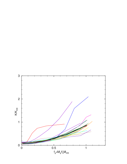
Figure 5: Dimensionless entropy profiles $K(M_{g})/K_{200}$ for twenty-four halos from a numerical simulation without radiative cooling or feedback. The objects were drawn from simulation L50+ described in Bryan & Voit (2001). They span a mass range from $2.5\times 10^{13}\,h^{-1}\,M_{\odot}$ to $3.5\times 10^{14}\,h^{-1}\,M_{\odot}$, yet they generally have nearly linear entropy distributions with the same normalization found in more massive clusters, $K(r_{200})\approx K_{200}$, with no significant trend in mass. A bold solid line shows the median profile.

This discrepancy between the entropy generated by smooth accretion and the entropy produced in simulations is even larger in groups because of their slower accretion rates. The logarithmic derivative $d\ln\eta/d\ln t$ for groups is only about half the large-cluster value (see Figure 1). According to equation (10), the dimensionless entropy $\hat{K}_{\rm sm}$ should correspondingly be $\sim$50% larger, approaching $\sim 3K_{200}$ at $f_{g}\sim 1$. Yet, the dimensionless entropy profiles of simulated groups remain similar to those of simulated clusters. Figure 5 shows entropy distributions for the twenty-four highest-mass objects in $\Lambda$CDM simulation L50+ of Bryan & Voit (2001). Except for a few outliers, these halos share a dimensionless entropy distribution similar to that of the more massive Santa-Barbara cluster, even though their masses range from $2.5\times 10^{13}\,h^{-1}\,M_{\odot}$ to $3.5\times 10^{14}\,h^{-1}\,M_{\odot}$.

2.5 Departures from Smooth Accretion

The most obvious explanation for the difference in normalization between the smooth accretion model and those derived from simulations and observations is that the accreting gas in a more realistic model would be lumpy, not smooth. Any inhomogeneity in the density of gas accreting onto a cluster tends to reduce the mean post-accretion entropy, as long as the velocity of the accreting gas remains unchanged. The reduction occurs because the postshock entropy scales as $v_{\rm ac}^{2}\rho_{1}^{-2/3}$ and the mass-weighted mean value of $\rho_{1}$ is larger if there is any inhomogeneity, anisotropy, or unsteadiness in the accretion flow (see Appendix B).

This sensitivity of the postshock entropy to the density distribution of incoming material means that the entropy normalization of a cluster or group reflects the lumpiness of the gas that accreted onto it. In Section 4 we will show that this effect may actually be important—the elevated normalization of entropy in groups suggests that accretion of baryons onto groups was smoother than accretion of baryons onto clusters. However, we will first continue with our analysis of smooth accretion in order to include preheating and cooling in the analytical model.

3 Smooth Accretion of Preheated Gas

Many authors have argued that preheating of gas that accretes onto a cluster is needed to explain the observed slope of the $L$–$T$ relation (e.g., Kaiser 1991; Evrard & Henry 1991; Navarro, Frenk, & White 1995; Cavaliere, Menci, & Tozzi 1997; Balogh et al. 1999; Ponman et al. 1999). Depending on how the analysis is done, the necessary amount of preheating ranges from $Tn_{e}^{-2/3}\sim 100\,{\rm keV}\,{\rm cm}^{2}$ to over $400\,{\rm keV}\,{\rm cm}^{2}$, corresponding to $K\sim 10^{33}\,{\rm erg\,cm^{2}\,g^{-5/3}}$ to $4\times 10^{33}\,{\rm erg\,cm^{2}\,g^{-5/3}}$ (but see § 4.1). If the preshock entropy level $K_{1}$ is comparable to $K_{\rm sm}$, then we can no longer assume that the accreting gas is pressureless. In particular, the Mach number of the accretion shock is $\stackrel{{\scriptstyle\propto}}{{\sim}}(K_{\rm sm}/K_{1})^{1/2}$, meaning that production of postshock entropy depends on the level of preheating.

In this section we derive an entropy jump condition that accounts for preheating and outline how preheating affects the position of the shock radius, suppressing the postshock entropy. Because radiative cooling can offset some of the effects of preheating, we also derive a simple approximation to treat cooling. Then, we add both preheating and cooling to our simple analytical entropy profiles and compare them with the numerically modeled entropy profiles of Tozzi & Norman (2001). Because the analytical profiles closely match the numerically computed ones, we conclude that our analytical model is a good representation of smooth accretion.

3.1 Entropy Jump Condition

A jump condition for entropy production when preheated gas passes through a shock can be derived from the jump conditions for other quantities. From the density jump condition, we get

$$v_{\rm in}=v_{1}-v_{2}=\frac{3}{4}\left(1-\frac{1}{{\cal M}^{2}}\right)v_{1}\;\;,$$ (11)

where $v_{1}$ and $v_{2}$ are the preshock and postshock gas velocities, respectively, in the rest frame of the shock, and $v_{\rm in}$ is the velocity of incoming gas relative to the postshock gas. The Mach number ${\cal M}=(3\rho_{1}v_{1}/5P_{1})^{1/2}$ of the shock is then determined by

$$\frac{({\cal M}^{2}-1)^{2}}{{\cal M}^{2}}=\frac{16}{15}\frac{\rho_{1}v_{\rm in}^{2}}{P_{1}}\;\;.$$ (12)

Noting that $K_{1}=P_{1}\rho_{1}^{-5/3}$ and setting $v_{\rm in}=v_{\rm ac}$, we obtain

$$\frac{({\cal M}^{2}-1)^{2}}{{\cal M}^{2}}=\frac{4^{8/3}}{5}\frac{K_{\rm sm}}{K_{1}}\;\;.$$ (13)

Solving this quadratic equation for the larger root gives

$${\cal M}^{2}=\frac{4^{8/3}}{5}\frac{K_{\rm sm}}{K_{1}}\left(\frac{1+q_{K}+\sqrt{1+2q_{K}}}{2}\right)\;\;,$$ (14)

where $q_{K}\equiv 10K_{1}/4^{8/3}K_{\rm sm}$.

Figure 6: Modification of postshock entropy owing to preheating. Accretion of cold gas produces a postshock entropy $K_{\rm sm}=v_{\rm ac}^{2}/3(4\rho_{1})^{2/3}$ in the high Mach-number limit. Preheating that raises the entropy of incoming gas to a preshock value $K_{1}$ weakens the shock but raises the postshock entropy $K_{2}$ above $K_{\rm sm}$ by an amount $\approx 0.84K_{1}$. The solid line in the upper panel shows $K_{2}/K_{1}$ as given by equation (15). The dotted line shows the postshock entropy $K_{\rm sm}/K_{1}$ one finds if preheating is ignored. The dashed line shows an approximate correction for preheating: $K_{2}\approx K_{\rm sm}+0.84K_{1}$. The lower panel more precisely shows the difference between $K_{2}$ and $K_{\rm sm}$.

Now we can express the jump conditions in terms of $K_{\rm sm}/K_{1}$,

$$\frac{P_{2}}{P_{1}} = 4^{5/3}\frac{K_{\rm sm}}{K_{1}}\left(\frac{1+\sqrt{1+2q_{K}}}{2}+\frac{2q_{K}}{5}\right)$$

$$\frac{\rho_{1}}{\rho_{2}} = \frac{1}{4}\left(1+\frac{3q_{K}}{1+q_{K}+\sqrt{1+2q_{K}}}\right)\;\;,$$

which lead to

$$K_{2} = K_{\rm sm}\left(\frac{1+\sqrt{1+2q_{K}}}{2}+\frac{2q_{K}}{5}\right)\;\;\;$$

$$\;\;\times\left(1+\frac{3q_{K}}{1+q_{K}+\sqrt{1+2q_{K}}}\right)^{5/3}\;\;.$$ (15)

In the limit $q_{K}\ll 1$, equivalent to $K_{\rm sm}/K_{1}\gg 0.25$, this expression reduces to $K_{2}\approx K_{\rm sm}+0.84K_{1}$ (see Figure 6; Dos Santos & Doré (2002) arrive at a similar approximation following a different route.) From this point of view, simply adding a constant value to the entropy profile produced without preheating, as in the shifted models of Voit et al. (2002), seems like a good representation of the effects of preheating.

3.2 Preheating and the Shock Radius

If the entropy of accreting gas substantially exceeds that which would be created by a shock, then we can no longer assume $\xi\approx 0.5$. Because the pressure just inside the shock front must balance the ram pressure of accreting gas, the position of the shock radius depends on both the current accretion rate and the internal structure of the cluster. When extra entropy, over and above that produced by cold accretion, is present within the cluster, the equilibrium shock radius is larger. If the extra entropy substantially exceeds $K_{\rm sm}$, then the equilibrium radius becomes so large that shock heating is essentially turned off.

Appendix A presents an approximate analytical solution for the equilibrium shock radius in terms of the associated shock-velocity parameter $\xi$ that applies when preheated gas smoothly accretes onto a cluster. Figure 7 shows the relation between $\xi$ and $M(t)$ arising from the accretion histories and concentration parameters used by Tozzi & Norman (2001). As in the numerical models of Tozzi & Norman (2001), the initial shock radius greatly exceeds the virial radius ($r_{\Delta}=r_{\rm ta}/2$) because the entropy of preheating, $K_{1}=3\times 10^{33}\,{\rm erg\,cm^{2}\,g^{-5/3}}$, is much larger than the characteristic entropy of the nascent dark-matter halo. Eventually, the halo’s gravity overcomes the effects of preheating, pulling the shock radius inward to a stable value of $\xi$. The more massive cluster ($10^{15}\,h^{-1}\,M_{\odot}$) achieves a larger value of $\xi\approx 0.45$ primarily because its faster accretion rate is more effective at compressing the gas internal to the shock front. In the less massive cluster ($10^{14}\,h^{-1}\,M_{\odot}$), accretion is more gradual, resulting in less compression and a smaller value of $\xi\approx 0.35$. For comparison, we also show solutions for $\xi$ using the accretion histories of § 2.3 but otherwise identical cluster parameters. In both cases, faster accretion produces a higher value of $\xi$.

Figure 7: Shock-radius parameter $\xi$ as a function of the accreted mass $\eta(t)=M(t)/M_{200}$. The solid lines show solutions for $\xi$ using the model developed in Appendix A for the cluster parameters of Tozzi & Norman (2001). The dotted lines show solutions found using the accretion histories of § 2.3 but otherwise identical cluster parameters. Lines at the upper left show clusters of mass $10^{15}\,h^{-1}\,M_{\odot}$; those at the lower right show clusters of mass $10^{14}\,h^{-1}\,M_{\odot}$. In all cases, the initial shock radius greatly exceeds the virial radius ($r_{\Delta}=r_{\rm ta}/2$) because the entropy of preheating ($K_{1}=3\times 10^{33}\,{\rm erg\,cm^{2}\,g^{-5/3}}$) grossly distends the intracluster medium. After the cluster’s gravity overcomes the entropy of preheating, the equilbrium value of $\xi$ is determined primarily by the accretion rate onto the cluster.

The constancy of $\xi$ in the shock-dominated regimes of these clusters is not trivial. On one hand, the rise in halo concentration with time tends to pull the shock radius slightly inward. On the other hand, the decrease in accretion rate with time allows the shock radius to slowly increase. In these particular models, the two tendencies nearly cancel. Note also that the model we are using is not a good representation for $\xi\ll 0.5$ because we have assumed that the time at which infalling gas reaches the shock radius is twice the time it took to reach its turnaround radius.

3.3 Correcting for Cooling

Radiative cooling can significantly modify the entropy distribution near the center of a cluster, if the entropy of preheating is not excessively large. One illustrative way to express the effects of radiative losses is with the following equation for the resulting change in entropy:

$$\frac{dK^{3/2}}{dt}=-\frac{3}{2}\frac{K_{c}^{3/2}(T)}{t_{0}}\;,$$ (16)

where

$$K_{c}(T)=\left[\frac{2}{3}\left(\frac{n_{e}n_{p}}{\rho^{2}}\right)\frac{T^{1/2}\Lambda(T)}{(\mu m_{p})^{1/2}}\right]^{2/3}t_{0}^{2/3}$$ (17)

is the entropy level at which constant-density gas at temperature $T$ radiates an energy equivalent to its thermal energy in the time $t_{0}$ and $\Lambda(T)$ is the standard cooling function. Figure 8 shows how $K_{c}(T)$ depends on $T$ in the models of Sutherland & Dopita (1993) for various metallicities. The solid line highlights $K_{c}(T)$ for a typical cluster metallicity of $\log Z/Z_{\odot}=-0.5$.

Figure 8: Threshold entropy for cooling within $t_{0}=15$ Gyr as a function of temperature and metallicity. The quantity $K_{c}(T)$ is defined in equation (17). Reading down from the top, the lines show $K_{c}(T)$ for metallicities of $\log Z/Z_{\odot}=0.5$, 0.0, -0.5, -1.0, -1.5, -2.0, 3.0, and zero metallicity, based on the cooling functions of Sutherland & Dopita (1993). The single solid line highlights the value of $K_{c}(T)$ for a typical cluster metallicity of $\log Z/Z_{\odot}=-0.5$.

In a simple spherical accretion model, a gas shell experiences no additional heat input after it has passed through a shock front. Gravitational compression can raise the temperature of the shell, but its entropy does not rise. Thus, radiative cooling inexorably lowers the entropy of the shell, resulting in

$$K_{\rm mod}(\eta)=\left[K_{2}^{3/2}(\eta)-K_{\rm rad}^{3/2}(\eta)\right]^{2/3}\;\;,$$ (18)

where

$$K_{\rm rad}(\eta)\equiv\left[\frac{3}{2t_{0}}\int_{t(\eta)}^{t_{0}}K_{c}^{3/2}(T)\,dt\right]^{2/3}\;\;.$$ (19)

The term $K_{\rm rad}(\eta)$ characterizes the entropy lost by the gas shell that accretes at time $t(\eta)$ after it passes through the accretion shock. In the comparisons that follow, we approximate $K_{\rm rad}(\eta)$ by setting $T$ equal to $T_{\phi}=GM\mu m_{p}/r_{\rm ta}$, the characteristic temperature of the dark matter halo at time $t$, which directly ties the integrand to the accretion history. We also assume a constant metallicity of $\log Z/Z_{\odot}=-0.5$.

3.4 Comparisons with Numerical Models

Having developed expressions for how preheating and radiative cooling affect the postshock entropy of smooth accreting gas, we are now in a position to compare our analytical accretion model with the numerical models of Tozzi & Norman (2001). Their standard models assumed an initial entropy $K_{1}=3\times 10^{33}\,{\rm erg\,cm^{2}\,g^{-5/3}}$ and a constant metallicity of $0.3Z_{\odot}$. The underlying cosmology was $\Lambda$CDM with $\Omega_{\rm M}=0.3$, $\Omega_{\Lambda}=0.7$, and $h=0.65$, so that $f_{b}=0.158$ and $t_{0}=14.5$ Gyr.

Figure 9: Entropy profiles for preheated gas that has accreted into a cluster with $M(t_{0})=10^{15}\,h^{-1}\,M_{\odot}$. The solid line shows the numerical model of Tozzi & Norman (2001). The long-dashed line shows the analytical model ($K_{\rm mod}$) from this paper, computed from the accretion history assumed by Tozzi & Norman (2001), including corrections for preheating and radiative cooling. The short-dashed line indicates the entropy profile ($K_{\rm sm}$) that results if these corrections are not applied. Dotted lines show $K_{1}$, the initial entropy of preheating, $K_{c}(T_{200})$ the cooling threshold of the final cluster, and the halo entropy scale $K_{200}$. The dot-dashed line shows $K_{\rm rad}$, the correction term for radiative cooling. Because both $K_{1}$ and $K_{\rm rad}$ are small compared to $K_{200}$, these corrections have only a minor effect on the global entropy profile outside the very center.

Figure 9 shows the comparison for a $10^{15}\,h^{-1}\,M_{\odot}$ cluster. In this case, the analytical model closely tracks the nearly linear behavior of the numerically computed profile at $f_{g}>0.1$. Outside the lowest-entropy regions, the corrections owing to preheating and radiative cooling are relatively small because $K_{1}$ and $K_{\rm rad}$ are both less than 10% of the cluster’s characteristic entropy. However, preheating is important early in the accretion history, when the characteristic entropy of the young halo is much smaller, and the relationship between preheating and cooling has important implications for the fate of the central gas.

Figure 7 shows that the first $\sim 5$% of the cluster’s gas accretes nearly isentropically because $\xi\ll 0.5$, so its entropy remains at the initial value of $K_{1}=3\times 10^{33}\,{\rm erg\,cm^{2}\,g^{-5/3}}$. After this gas accretes, it is subject to radiative cooling. The approximate cooling model of § 3.3 gives $K_{\rm rad}\approx 3.5\times 10^{33}\,{\rm erg\,cm^{2}\,g^{-5/3}}$ for the earliest gas to accrete, $\sim 15$% higher than the entropy of preheating. (Note that the cooling threshold $K_{c}(T_{200})$ of cluster gas at time $t_{0}$ closely corresponds to the integral for $K_{\rm rad}$.) The entropy of the innermost gas therefore drops to zero, implying a condensed fraction $\sim 5$%, which is ten times greater than the $\sim 0.5$% condensed fraction in the Tozzi & Norman (2001) model. Yet, if the cooling rate in the analytical model were $\sim 20$% smaller, or preheating were $\sim 20$% greater, the condensed fraction would be zero. This underscores the importance of accounting for entropy produced by internal feedback following cooling and condensation of intracluster gas (e.g., Voit & Bryan 2001).

Figure 10: Entropy profiles for preheated gas that has accreted into a cluster with $M(t_{0})=10^{14}\,h^{-1}\,M_{\odot}$. Lines have the same meanings as in Figure 9. Because the entropy of preheating is relatively significant, the accretion radius is initially much larger than the virial radius (see Figure 7), and the first third of the cluster’s gas accretes isentropically. After a strong shock develops, the entropy profile exceeds $K_{\rm sm}$ by $\approx 0.84K_{1}$. Because $K_{\rm rad}$ is not much less than $K_{1}$, radiative cooling significantly diminishes the central entropy.

Preheating has a much more significant impact on the $10^{14}\,h^{-1}\,M_{\odot}$ cluster, yet the analytical model remains a good match to the numerical model. In this case, over 30% of the gas accretes isentropically, while $\xi\ll 0.5$ (see Figure 7). Even after the accretion shock strengthens, there is still a significant constant offset ($\approx 0.84K_{1}$) between $K_{\rm sm}$ and the Tozzi & Norman (2001) model. Cooling diminishes the final entropy of the gas that accreted isentropically, and this decrease is again slightly larger in the analytical model than in the numerical model. Note also that $K_{c}(T_{200})$ remains a good approximation to $K_{\rm rad}$ for the central gas.

Figure 11: Entropy profiles for preheated gas that has accreted into a cluster with $M(t_{0})=10^{13}\,h^{-1}\,M_{\odot}$. Lines have the same meanings as in Figure 9. In this case, the entropy of preheating exceeds the characteristic entropy of the final cluster, so the accretion radius never approaches the virial radius. Accretion is therefore virtually isentropic. As in the $10^{13}\,h^{-1}\,M_{\odot}$ cluster, radiative cooling significantly lowers the central entropy.

The characteristic entropy of a $10^{13}\,h^{-1}\,M_{\odot}$ halo is so small that $3\times 10^{33}\,{\rm erg\,cm^{2}\,g^{-5/3}}$ of preheating dominates everything. The shock radius never approaches the virial radius, so all the gas accretes isentropically. Because $K_{\rm rad}\approx 0.5K_{1}$ for the earliest gas to accrete, cooling diminishes the central entropy by $\sim 25$%. Again, the analytical model calls for slightly more cooling than the numerical model.

In all three cases, our approximate analytical model for smooth accretion seems to represent with reasonable accuracy all the important processes operating in the numerical models. The analytical models show that preheating can suppress radiative cooling in a given mass shell if $K_{\rm sm}+0.84K_{1}$ exceeds $K_{\rm rad}\approx K_{c}(T_{200})$. However, the cores of these objects become isentropic if $K_{1}$ is comparable to $K_{200}$ and larger than $K_{\rm rad}$ (see Figures 10 and 11).

3.5 Inhomogeneous Preheated Gas

What effect does inhomogeneity have on accretion of preheated gas? According to § 3.1, the postshock entropy of preheated gas is

$$K_{2}\approx\frac{v_{\rm in}^{2}}{3(4\rho_{1})^{2/3}}+0.84K_{1}$$ (20)

As long as the shock velocities $v_{\rm in}$ are comparable to the accretion velocity $v_{\rm ac}$, the postshock entropy will depend primarily on the preshock density $\rho_{1}$ and the preshock entropy $K_{1}$. When we consider how preheating affects the case of lumpy, hierarchical accretion, the second term containing $K_{1}$ is relatively straightforward to apply and produces a correction no greater than the entropy of preheating. However, if preheating can significantly smooth the accreting gas, substantially lowering the mean mass-weighted preshock density, then the increase in postshock entropy owing to the $v_{\rm in}^{2}/3(4\rho_{1})^{2/3}$ term can be considerably larger than $K_{1}$. We will consider some observational evidence for this effect in section 4.

Notice also that equation (20) does not explicitly depend on the temperature of the preheated gas. We are choosing to focus on entropy and density, rather than on preshock temperature, because this way of casting the problem implicitly accounts for preshock heating owing to adiabatic compression. In fact, focusing on preshock temperature can be misleading because adiabatic heating actually decreases the postshock entropy of an accreting gas blob; compression increases the preshock density, lowering $K_{\rm sm}$ without changing $K_{1}$. The entropy gain across the shock is smaller because the preshock temperature is larger than it would have been without the compression, so the heat input released by thermalization of the incoming kinetic energy produces less entropy. Thus, the postshock entropy is more closely related to the preshock density distribution than to the preshock temperature distribution.

4 Evidence for Smoothed Accretion

The results of the previous two sections imply that the impact of preheating on lumpy accretion qualitatively differs from its impact on smooth accretion. Entropy input preceding smooth accretion suppresses entropy production at the accretion shock because it pushes the accretion radius beyond the virial radius (e.g., Balogh et al. 1999; Tozzi & Norman 2001; § 3.2). If the entropy of preheating exceeds the characteristic entropy of the halo, then smooth accretion becomes virtually adiabatic, leading to a nearly isentropic entropy distribution. However, dense lumps of accreting gas will not necessarily be prematurely halted by the distended intracluster medium, so it is not clear that entropy production by lumpy accretion will be diminished in quite the same way.

On the contrary, preheating might actually enhance entropy generation over what would normally be produced in the lumpy accretion mode. Because preheating tends to lower the density of gas within small halos, it smooths the density distribution accreting onto larger halos, increasing the efficiency with which accretion shocks generate entropy. If preheating ejects a majority of the gas from small halos, then this effect might be strong enough to cause a transition from lumpy accretion to smooth accretion on the mass scale of groups. In that case, smooth accretion onto groups would produce an entropy normalization $\sim$2-3 times higher than that expected from self-similar scaling of clusters. Furthermore, if the initial level of preheating ($K_{1}$) is relatively small compared to the characteristic entropy of the final halo ($K_{200}$), then the final halo need not have a substantial isentropic core.

This section examines some intriguing pieces of observational evidence suggesting that preheating alters the entropy distributions of groups primarily by smoothing the gas that accretes onto them. Thus, the large amounts of preheating needed to explain the $L$-$T$ relation in the case of isentropic groups might be unnecessary. First, we show that groups with flat entropy gradients cannot simultaneously be consistent with both the observed $L$-$T$ relation and observations of core entropy. Polytropic models of groups with an effective adiabatic index $\gamma_{\rm eff}\approx 1.2$ are more consistent with these constraints, indicating that the entropy gradients of groups are similar to those of clusters. Then, we show that these polytropic models imply entropy levels at the virial radii of groups that exceed the maximum value of $K(r_{200})\approx K_{200}$ expected from lumpy accretion, a conclusion supported by recent measurements of entropy at the outskirts of groups (Finoguenov et al. 2002). The excess entropy implied by observations is similar to the amount expected from smooth accretion onto groups, perhaps indicating a transition from lumpy accretion to smooth accretion at a mass scale $\sim 10^{14}\,h^{-1}\,M_{\odot}$ owing to preheating in smaller halos.

4.1 Entropy Gradients of Groups

The relationship between the X-ray luminosities and temperatures of groups and clusters has long been assumed to indicate an early episode of preheating, but the necessary amount of preheating is a matter of some debate. Purely gravitational structure formation calls for $L\propto T^{2}$ (e.g., Kaiser 1986), yet observations show $L\propto T^{2.5-3}$ (e.g., Edge & Stewart 1991). This steepening of the $L$-$T$ slope requires some sort of non-gravitational modification of the core entropy (Kaiser 1991; Evrard & Henry 1991; Bower 1997; Voit et al. 2002).

Some models are able to fit this relation with a core entropy $\sim 100$-$150\,{\rm keV\,cm^{2}}$ $(\sim 1.0-1.5\times 10^{33}\,{\rm erg\,cm^{3}\,g^{-5/3}}$) (e.g., Cavaliere et al. 1997, 1998, 1999; Voit & Bryan 2001; Bialek, Evrard, & Mohr 2001; dos Santos & Doré 2002). Other models require $\sim 200$-$400\,{\rm keV\,cm^{2}}$ $(\sim 2.0$-$4.0\times 10^{33}\,{\rm erg\,cm^{3}\,g^{-5/3}}$) (e.g., Balogh et al. 1999; Tozzi & Norman 2001; Babul et al. 2002). The primary difference between these two classes of models is that those requiring large amounts of preheating have isentropic entropy profiles extending to a large fraction of the virial radius, while those requiring less central entropy assume a significant entropy gradient throughout the group.

We can quantify this difference using the polytropic models described by equations (A3) through (A9) of Appendix A. These models require two boundary conditions and an effective polytropic index $\gamma_{\rm eff}$. For this application, we set one boundary condition so that the pressure at $r_{200}$ is the same for all models, and we choose that pressure to be equal to the $\gamma_{\rm eff}=1.2$ case with a total gas mass $f_{b}M_{200}$ within $r_{200}$. For the other boundary condition we fix the entropy at at $0.1r_{200}$. Each model is therefore determined by the halo mass $M_{200}$, the halo concentration parameter $c_{200}$, the polytropic index $\gamma_{\rm eff}$, and the core entropy $K_{0.1}\equiv K(0.1r_{200})$. For each halo mass, we consider a set of polytropic models with $\gamma_{\rm eff}=1.2$ and a set of isentropic models ($\gamma_{\rm eff}=5/3$).

Figure 12 shows the luminosity-temperature relation we need to reproduce. We plot the quantity $L_{X}/T_{\rm lum}^{3}$, where $T_{\rm lum}$ is the luminosity-weighted temperature, because it is nearly constant at $\sim 1.5\times 10^{42}\,h^{-3}\,{\rm erg\,s^{-1}\,keV^{-3}}$ for $T_{\rm lum}\gtrsim 1\,{\rm keV}$ and a little bit smaller below that temperature. Figure 13 shows the same quantity drawn from the polytropic models for two different halo masses, $M_{200}=5\times 10^{13}\,h^{-1}\,M_{\odot}$ and $M_{200}=1\times 10^{13}\,h^{-1}\,M_{\odot}$ with luminosity-weighted temperatures of $T_{\rm lum}\approx 1.4\,{\rm keV}$ and $T_{\rm lum}\approx 0.5\,{\rm keV}$, respectively. The halo concentration is $c_{200}=10$ in all cases and we truncate the integrations for $L_{X}$ and $T_{\rm lum}$ at the virial radius.

Figure 12: Luminosity-temperature relation for groups and clusters in terms of $L_{X}/T_{\rm lum}^{3}$. Solid triangles show measurements of clusters with insignificant cooling flows compiled by Arnaud & Evrard (1999). Open squares show cooling-flow corrected measurements by Markevitch (1998). Solid circles show group data from Helsdon & Ponman (2000). Note that the quantity $L_{X}/T_{\rm lum}^{3}$ remains roughly constant at $\sim 1.5\times 10^{42}\,h^{-3}\,{\rm erg\,s^{-1}\,keV^{-3}}$ (upper dotted line), dipping to slightly lower levels ($\sim 0.5\times 10^{42}\,h^{-3}\,{\rm erg\,s^{-1}\,keV^{-3}}$ (lower dotted line) below $\sim 1$ keV.

Figure 13: Dependence of $L_{X}/T_{\rm lum}^{3}$ on the entropy scale $K_{0.1}$ at $0.1r_{200}$ in polytropic models. Tracks are shown for two different halo masses: $5\times 10^{13}\,h^{-1}\,M_{\odot}$ (solid lines) and $1\times 10^{13}\,h^{-1}\,M_{\odot}$ (dashed lines). Each pair of tracks corresponds to different effective polytropic index. The upper tracks represent isentropic models ($\gamma_{\rm eff}=5/3$), and the lower tracks represent polytropic models with an entropy gradient similar to those observed in clusters ($\gamma_{\rm eff}=1.2$). The halo concentration is $c_{200}=10$ in all models, and the pressure at $r_{200}$ is the same in all models. Dotted lines indicate the same values of $L/T^{3}$ as in Figure 12. One can reproduce the observed $L/T^{3}$ ratio with either $\gamma_{\rm eff}\approx 1.2$ and $K_{0.1}\approx 130\,{\rm keV\,cm^{2}}$ or with $\gamma_{\rm eff}\approx 5/3$ and $K_{0.1}\approx 350\,{\rm keV\,cm^{2}}$.

Comparing Figure 12 with Figure 13 shows that both the isentropic models and the $\gamma_{\rm eff}=1.2$ models can reproduce the $L$-$T$ relation, but the isentropic models call for higher levels of core entropy. The reason for this behavior is that the density profile of the isentropic models is shallower than $\rho\propto r^{-3/2}$, so that $L_{X}$ is dominated by emission from near the virial radius. The overall luminosity is then set by the entropy level in the outer regions of the group. Conversely, when $\gamma_{\rm eff}\approx 1.2$, the density profile is steeper than $\rho\propto r^{-3/2}$. The inner regions then dominate the total luminosity, and the core entropy can be lower because a smaller amount of gas produces most of the emission. Because observations of core entropy in $\sim$1 keV halos indicate that $K_{0.1}\approx 100$-$150\,{\rm keV\,cm^{2}}$ (Ponman et al. 1999), models with significant entropy gradients, consistent with $\gamma_{\rm eff}\sim 1.2$, are probably closer to the actual entropy profiles of groups.

4.2 Entropy at the Outskirts

The preceding analysis suggests that groups are not isentropic but instead have entropy gradients more like those observed in clusters. This finding, when coupled with the elevated levels of core entropy observed in groups (e.g. Ponman et al. 1999), implies that entropy at the outskirts of groups must also be elevated above the predictions of pure gravitational structure formation. If the shape of the entropy gradient is unchanged, then the main difference between groups and clusters must be in the normalization of the entropy gradient rather than its slope.

Figure 14 shows the scaled entropy $K/K_{200}$ at $r_{200}$ implied by polytropic models having different halo masses but a fixed value of core entropy $K_{0.1}=150\,{\rm keV}\,{\rm cm^{2}}$. In polytropic models with $\gamma_{\rm eff}=1.2$ and this value of core entropy, the implied entropy at $r_{200}$ is $\sim 2$-4 times larger than $K_{200}$ over the mass range $10^{13}\,h^{-1}\,M_{\odot}$ to $10^{14}\,h^{-1}\,M_{\odot}$. For comparison, we also show the implied entropy for an effective polytropic index of $\gamma_{\rm eff}=1.3$, which agrees less well with the observational constraints. In that case, the outer entropy levels drop to $\sim 1$-3 times $K_{200}$. However, the entropy levels at $K_{200}$ in groups simulated without preheating or cooling are rarely much greater than $K_{200}$, with no significant trend in mass (see Figure 5). Notice that these entropy enhancements are quite difficult to produce by heat input alone. The value of $K_{200}$ for a $10^{14}\,h^{-1}\,M_{\odot}$ halo is $\sim 700\,{\rm keV}\,{\rm cm}^{2}$, so doubling that entropy would require an enormous amount of heat.

Figure 14: Entropy at $r_{200}$ in polytropic models with core entropy $K_{0.1}=150\,{\rm keV}\,{\rm cm^{2}}$. The polytropic indices ($\gamma_{\rm eff}\sim 1.2-1.3$) consistent with both the $L$-$T$ relation and the observed core entropy of groups $\sim 100$-$150\,{\rm keVcm^{2}}$, imply $K(r_{200})\sim 2$-$3K_{200}$.

Direct observations of entropy at the outskirts of a few groups support the idea that groups have significant entropy gradients and higher maximum entropy levels than predicted by self-similar models that do not include non-gravitational processes. Finoguenov et al. (2002) determined $Tn_{e}^{-2/3}$ as a function of radius in several groups using ASCA and ROSAT data and compared them with the entropy gradients of more massive systems. After dividing these gradients by $M_{500}^{2/3}$ to remove the dependence on mass scale, they found that the outer entropy levels of groups exceeded those in clusters by a similar factor of 2-3, with a large scatter.

Finoguenov et al. (2002) interpreted this excess entropy as a $\sim 400\,{\rm keV\,cm^{2}}$ “entropy ceiling” produced entirely by non-gravitational heating owing to galactic winds. In this interpretation, the entropy gradient results from a gradual rise in the entropy of the intergalactic medium external to a group before it accretes onto the group. For this level of entropy to be produced by supernovae, the energy injection must occur with near 100% efficiency at redshift $z\sim 3$ into regions of relatively low overdensity ($\sim 5\rho_{\rm cr}$).

4.3 A Smooth-Accretion Interpretation

We would like to offer another interpretation of this apparent entropy excess that is based on the smooth accretion models developed in this paper. Relatively small amounts of preheating ($\lesssim 100\,{\rm keV\,cm^{2}}$) can eject much of the gas from the smaller halos that accrete onto a group or a large elliptical galaxy at late times, making the accreting gas more homogeneous. This more modest level of preheating can therefore break self-similarity by allowing the group to generate most of its entropy through smooth accretion. The general shape of the entropy profile remains similar to the lumpy-accretion case because it is determined by the accretion history (§ 2.3), but its normalization is boosted because the mean density of incoming gas is reduced (§ 2.5).

In the limit of perfectly smooth accretion, equation (10) implies that

$$\frac{K(r_{200})}{K_{200}}\approx 2.6\,\left(\frac{d\ln M}{d\ln t}\right)^{-2/3}\;\;,$$ (21)

assuming that $H_{0}t_{0}$, $2\xi$, and $\eta$ are all $\approx 1$. The enhancement of entropy at $r_{200}$ relative to expectations from hierarchical accretion is larger for smaller halos because it depends on the mass accretion rate. Inserting the $d\ln M/d\ln t$ values at $t=t_{0}$ from Figure 1 into equation (21) yields $K(r_{200})/K_{200}\approx 3.5$ for $10^{13}\,h^{-1}\,M_{\odot}$, $\approx 2.4$ for $10^{14}\,h^{-1}\,M_{\odot}$, and $\approx 1.7$ for $10^{15}\,h^{-1}\,M_{\odot}$. Note also that smooth accretion can increase the effectiveness of preheating at limiting condensation in groups, as the initial entropy input needed to smooth the accreting gas is strongly amplified at the accretion shock.

5 The Puzzle of Entropy Normalization

Groups and clusters appear to have similar entropy profiles, consistent with an effective polytropic index $\gamma_{\rm eff}\sim 1.2$ at large radii. However, the normalizations of those profiles cannot scale with $K_{200}\propto M_{200}^{2/3}$, as they would if they were determined by purely gravitational processes. Instead, the relationship between entropy normalization and halo mass is somewhat shallower, quite possibly because preheating has partially smoothed the intergalactic medium. Thus, we would like to understand more quantitatively how entropy production depends on the homogeneity of accreting gas.

The normalization of intracluster entropy in the smooth-accretion limit is relatively simple to calculate (see § 2), but the physics that sets the normalization during lumpy accretion is more complex. This section outlines some of the physical processes that might govern entropy production by lumpy accretion. We first present a naive model for merger shocks in which all the accreting gas belongs to virialized subhalos and all the incoming kinetic energy is thermalized through merger shocks within those subhalos. This naive model fails to produce the required amount of entropy, implying that either (1) the preshock density distribution and perhaps the accretion velocity assumed in the naive model poorly represent reality, or (2) some of the incoming kinetic energy is thermalized within the intracluster medium of the main halo. One way to account for the first possibility is to adjust the preshock density distribution, and we present an illustrative example involving power-law density distributions. The second possibility implies that lumpy accretion provides a distributed source of heating throughout a cluster, and we conclude the section by identifying the hallmarks of distributed heating and suggesting how to quantify it in numerical simulations.

5.1 Naive Merger Shocks

The accretion process usually envisioned in semi-analytic models of cluster formation calls for all the accreting gas to lie within a subhalo of some kind, even if many of those subhalos sit below the practical resolution limit of the calculation (e.g., Wu, Fabian, & Nulsen 2000; Bower et al. 2001). In a self-consistent semi-analytical model one would like to track how entropy develops as these subhalos collide and merge with the main halo and to calculate the density configuration of the new halo from that evolving entropy distribution (e.g., Balogh et al. 2003, in preparation). Instead, the density distribution is typically assumed to settle into a polytropic or $\beta$-model configuration similar to observed density profiles, with a core temperature equal to the virial temperature. Here we show that accretion shocks within discrete, accreting subhalos do not generate enough entropy to reproduce the characteristic entropy profile of a cluster.

If the mean gas density within each of the accreting subhalos is $\Delta f_{b}\rho_{\rm cr}$ and strong shocks thermalize all the kinetic energy of accretion within those subhalos as they cross the virial radius of the main halo, then for $\xi\approx 0.5$ we find that the mean postshock entropy of gas accreting at time $t$ is

$$\bar{K}(t) \approx \left(\frac{\rho_{1}}{\Delta f_{b}\rho_{\rm cr}}\right)^{2/3}K_{\rm sm}(t)$$ (22)

$$\approx \left[\frac{1}{3}\left(\frac{2}{\Delta}\right)^{1/2}(Ht)^{-1}\frac{d\ln M}{d\ln t}\right]^{2/3}K_{\rm sm}(t)\;\;.$$

The cosmologies and accretion histories considered here give $\bar{K}(t)\sim 0.1(\Delta/200)^{-1/3}K_{\rm sm}(t)$, several times smaller than the value found in the simulations and observations. According to § 3.1, about 84% of the preshock entropy in the subhalos should be added to $\bar{K}$, but this does not come close to fixing the problem unless the accreting halos are similar in size to the main halo, which is rare during the formation of a large cluster.

This postshock entropy deficit can be recast in terms of the shock velocity needed to rectify it. Suppose that the accreting subhalos have gas density distributions similar to that of the main halo. Because the gas temperature in the main halo is $\approx GM\mu m_{p}/2r_{\Delta}$, boosting the entropy distribution of the subhalo’s gas to match that of the main halo requires a shock velocity

$$v_{\rm sh} \approx \left[\frac{3\cdot 4^{2/3}}{2}\frac{GM}{r_{\Delta}}\right]^{1/2}$$

$$\approx 2v_{\rm ac}\;\;,$$ (23)

where $v_{\rm ac}$ is the infall velocity at radius $r_{\Delta}=r_{\rm ta}/2$. A gas blob entering a cluster with an NFW potential would need to fall unimpeded from its turnaround radius to $\lesssim 0.25r_{\Delta}$ before it reached a velocity $\approx 2v_{\rm ac}$. However, in the naive model we have outlined, infalling blobs do not fall so far toward the center of the main halo before being shocked and disrupted. If a dense lump of accreting gas does fall this far, then dissipation of its kinetic energy through shocks and turbulence is also quite likely to heat the main halo’s gas. We consider how this mechanism affects entropy generation in § 5.3.

5.2 Adjusted Merger Shocks

If one retains the assumption that merger shocks thermalize all the incoming energy within the accreting gas, then then one must adjust the incoming density distribution and perhaps raise the shock velocity. Striking the proper blend of smooth accretion and lumpy accretion would then yield the correct entropy level. To illustrate this idea, we briefly outline a case in which the accreting gas fills the accreting volume instead of being confined to regions with mean density $\sim\Delta f_{b}\rho_{\rm cr}$.

Suppose that the preshock density of accreting gas is distributed like a power law. Define $f(\rho)d\rho$ to be the fraction of accreting gas with density between $\rho$ and $\rho+d\rho$, so that $f(\rho)=(p-1)\rho_{\rm min}^{p-1}\rho^{-p}$ for a power-law index $p>1$. If we then assume that all the gas accreting at a given time shocks at the same accretion radius, we can integrate $\rho^{-2/3}f(\rho)d\rho$ to find the mean entropy of gas accreted at time $t$:

$$\bar{K}(t)=\frac{p-1}{p-\frac{1}{3}}\left(\frac{\rho_{1}}{\rho_{\rm min}}\right)^{2/3}K_{\rm sm}(t)\;\;.$$ (24)

If we further assume that the accreting gas fills the available volume, then $\rho_{1}/\rho_{\rm min}=p/(p-1)$ and

$$\bar{K}(t)=\frac{p^{2/3}(p-1)^{1/3}}{p-\frac{1}{3}}K_{\rm sm}(t)\;\;.$$ (25)

The power-law index $p$ is directly related to the density distribution within an accreting subhalo. In particular, for $\rho(r)\propto r^{-q}$, we have $p=3/q$. The case of extended singular isothermal spheres accreting onto the main halo therefore corresponds to $p=3/2$, and we get $\bar{K}\approx 0.89K_{\rm sm}(t)$. In the limit of small $q$ and large $p$, the incoming density distribution is nearly uniform, and $\bar{K}\approx K_{\rm sm}(t)$. However, $\bar{K}$ grows arbitrarily small in the limit of $q\rightarrow 3$ and $p\rightarrow 1$, in which case the majority of the gas becomes concentrated at high density. Thus, for some value of $q\lesssim 3$, the mean postshock entropy has the desired value.

This calculation implies that one can specify a preshock density distribution that yields the correct postshock entropy distribution after passing through an accretion shock. However, this model for entropy production is not necessarily the solution to the entropy normalization puzzle. In order to test it, one would need to measure the density distribution and infall velocity of baryonic material accreting onto a numerically simulated cluster and then compute the postshock entropy distribution implied by this model.

5.3 Distributed Heating

An alternative solution to the entropy normalization problem depends on an important qualitative difference between smooth accretion and lumpy accretion. Smooth accretion thermalizes all the incoming kinetic energy at the accretion shock, within gas that has just accreted. After a gas shell has become part of the intracluster medium, its entropy is no longer affected by the smooth-accretion process. However, dense lumps of accreting gas can penetrate the virial radius without substantially decelerating. They subsequently move through the main cluster, stirring up turbulence and stimulating shocks within the main cluster’s gas. These processes continue until either drag saps all of the dense lump’s kinetic energy or hydrodynamic instabilities tear the dense lump apart.

The recently observed presence of cold fronts in clusters (Markevitch et al. 2000; Vikhlinin, Markevitch, & Murray 2001) suggests that dense subhalos can remain coherent for quite a long time before blending with the rest of the intracluster medium. Thus, much of the incoming kinetic energy of lumpy accretion may ultimately be deposited into the pre-existing intracluster medium as the disturbances stirred up by the accreting lumps dissipate and thermalize (see e.g., Gomez et al. 2002). If that is the case, then accretion provides a distributed source of heating that adds entropy to the entire intracluster medium, not just to gas that has recently accreted.

Here we examine some crucial differences between entropy production through smooth accretion and entropy production through distributed heating. First we assess the amount of entropy growth that lumpy accretion needs to generate in order to maintain the self-similar entropy profiles observed in simulations and in hot clusters. Then we examine the implications of heating the existing intracluster medium through lumpy accretion, showing that the source of condensing low-entropy gas in the lumpy-accretion mode is different from its origin in the smooth-accretion mode. If distributed heating is important, then much of the core gas in present-day clusters may come from the cores of subhalos that accrete at $\sim 0.5t_{0}$. One can assess the importance of distributed heating by tracking the $K(t)$ trajectories of Lagrangian gas parcels in numerical simulations after they accrete onto a cluster.

5.3.1 Self-Similar Entropy Growth

One notable feature of numerically modelled clusters in simulated CDM-like cosmologies is their near self-similarity. The dark-matter potential wells approximately follow the NFW density profile, and the main systematic devations from self-similarity can be characterized with a halo concentration parameter that increases with decreasing halo mass (e.g., Navarro et al. 1997). This dependence on halo mass comes about because smaller halos tend to accumulate their mass earlier in time, when the mean density of the universe is larger (Navarro et al. 1997; Bullock et al. 2001; Eke, Navarro, & Steinmetz 2001). Numerical models including hydrodynamics also show that the baryonic density and temperature profiles in the absence of non-gravitational heating and cooling processes closely track the analogous dark-matter profiles, except in the very center (e.g., Navarro, Frenk, & White 1995; Eke et al. 1998; Frenk et al. 1999). Therefore, whatever processes are responsible for entropy growth during hierarchical structure formation act to preserve this near self-similarity.

If clusters were precisely self-similar, then their properties would be entirely determined by their mass $M$ and the time of observation, which determines the mean mass density $\Delta\rho_{\rm cr}$ within the cluster. According to the simple spherical infall model of § 2.2, the turnaround radius of matter accreting at time $t$ is $r_{\rm ta}=(2GMt^{2}/\pi^{2})^{1/3}$ and it falls through the virial radius ($r_{\rm ta}/2$) with a kinetic energy per particle $T_{\phi}=GM\mu m_{p}/r_{\rm ta}$. (These expressions are strictly true only if $\Lambda=0$, but they are accurate to within 10% for $\Lambda$CDM with $\Omega_{\Lambda}=0.7$.) Because the mean density within the virial radius is $3\pi/Gt^{2}$, the entropy scale associated with a cluster’s baryons is

$$K_{\phi}=\frac{1}{2}\left(\frac{2G^{2}}{3f_{b}}\right)^{2/3}(Mt)^{2/3}\;\;.$$ (26)

The dimensionless entropy distribution function $K(M_{g})/K_{\phi}$ would then be the same for all clusters.

One can integrate over this distribution to find the total classical thermodynamic entropy of a cluster’s baryons,

$$S(M,t)=\frac{f_{b}M}{\mu m_{p}}\left[\ln(Mt)+{\rm const.}\right]\;\;,$$ (27)

where the details of the self-similar distribution function are absorbed within the constant term. If the main halo accretes a subhalo of mass $\delta M\ll M$ during the time interval $\delta t\ll t$, then the entropy of the entire system, including the pre-accretion entropy of the subhalo’s baryons, rises by

$$\delta S = S(M+\delta M,t+\delta t)-S(M,t)$$

$$\;\;\;\;\;\;\;\;\;-\;S(\delta M,t)$$

$$= \frac{f_{b}\delta M}{\mu m_{p}}\left[1+\frac{M}{t}\frac{\delta t}{\delta M}+\ln\left(\frac{M}{\delta M}\right)\right]\;\;.$$ (28)

The first two terms in the lower expression correspond to the heat input needed to maintain self-similarity in the merged system, which presumably comes from thermalization of incoming kinetic energy. The third term corresponds to the entropy associated with raising the subhalo’s gas to the temperature of the main halo. The most efficient way to increase the entropy of that gas is to raise its temperature while keeping its density constant, perhaps through conduction of heat from the main cluster facilitated by rapid mixing. However, the subhalo’s baryons are more likely to be compressed or shock heated before mixing with the main intracluster medium, in which case a portion of the third term corresponds to thermalization of incoming kinetic energy within the subhalo’s gas.

Smooth accretion achieves self-similarity in a different way. From equation (10) it is evident that cold accretion can produce self-similar clusters as long as $\zeta\equiv d\ln M/d\ln t$ is the same for all clusters; the entropy profile produced by smooth accretion for constant $\zeta$ is $K(M_{g},t)=K_{\rm sm}(t)[M_{g}/f_{b}M(t)]^{2/3+2/3\zeta}$. In that case, the classical thermodynamic entropy of a cluster’s baryons is

$$S=\frac{f_{b}M}{\mu m_{p}}\left[\ln K_{\rm sm}^{3/2}-\left(1+\frac{1}{\zeta}\right)+s_{0}\right]\;\;,$$ (29)

which explicitly includes the constant term arising from the cluster’s internal structure. Smooth accretion of gas mass $f_{b}\delta M$ with pre-accretion entropy $K_{1}\ll K_{\rm sm}$ during a time interval $\delta t$ therefore adds

$$\delta S=\frac{f_{b}\delta M}{\mu m_{p}}\left[\frac{3}{2}\ln\left(\frac{K_{\rm sm}}{K_{1}}\right)\right]$$ (30)

to the thermodynamic entropy of the whole accreting system, after the initial entropy of the accreting gas has been subtracted. The entropy increase in this case is due entirely to shock heating of incoming gas at the accretion shock, and there are no additional heating terms.

5.3.2 Implications of Accretion Heating

The preceding analysis suggests that hierarchical merging produces entropy exceeding the amount needed to raise the accreting gas to the temperature of the original halo. A detailed accounting of how this heating occurs is beyond the scope of this paper, but we would like to suggest a qualitative picture that can be tested and refined with numerical simulations. Here we construct a toy model for distributed heating owing to accretion and show how it affects the evolution of the intracluster entropy distribution. If distributed heating is the dominant mode of entropy growth, then the entropy of gas deep within a cluster should rise with time, possibly compensating for some of the radiative cooling of the cluster core.

Let the rate at which accretion deposits heat energy into the intracluster medium be $\epsilon T_{\phi}f_{b}\dot{M}/\mu m_{p}$. If this energy deposition rate were equal to the rate at which kinetic energy passes through the virial radius, then we would have $\epsilon=1$. However, accreting gas that is denser than gas at the virial radius plunges to smaller radii, gaining additional energy to be thermalized as it descends into the cluster. A dense gas blob eventually comes to rest when its entropy equals that of the surrounding gas. Thus, the total rate of heat input owing to lumpy accretion might be somewhat larger than the rate at which kinetic energy flows through the virial radius, allowing $\epsilon$ to exceed unity.

Distributing this heat input equally among all the cluster’s gas particles leads to the following expression for the evolution of entropy with time within a Lagrangian gas parcel, including radiative cooling:

$$\frac{d\ln K^{3/2}}{dt}=\frac{\epsilon T_{\phi}}{T}\frac{d\ln M}{d\ln t}\frac{1}{t}-\frac{3}{2}\frac{K^{3/2}_{c}(T)}{K^{3/2}}\frac{1}{t_{0}}\;.$$ (31)

A more general model could be constructed by allowing $\epsilon$ to depend on $K$, thereby accounting for inhomogeneities in heat input. The mean value of $\epsilon$, integrated over time, and its spatial variations within a cluster would be interesting to measure in numerical simulations of hierarchical merging.

Figure 15: Change in entropy with time in the intracluster medium of the main halo owing to distributed heating and radiative cooling. The dotted lines show how Lagrangian gas parcels move through the $K$-$t$ plane, according to equation 31 with $\epsilon=1+(d\ln M/d\ln t)^{-1}$ and $T=T_{\phi}$. The solid line indicates the characteristic entropy $K_{\phi}(t)$ of the growing dark-matter halo. The short-dashed line gives $K_{\rm sm}(t)$ for $\xi=0.5$ and no preheating. The long-dashed line shows the threshold $K_{\rm th}$ below which a gas parcel is destined to condense by $t=t_{0}$. The dot-dashed line shows the cooling threshold $K_{c}(T_{\phi})$ corresponding to the characteristic temperature $T_{\phi}(t)$ of the halo. Because of the heat input generated by accretion, the entropy of the intracluster medium can increase with time, amplifying the effects of early entropy input and reducing the amount of gas that condenses by $t=t_{0}$.

Figure 16: Change in entropy with time in the intracluster medium of the main halo owing to radiative cooling only. The lines have the same meanings as in Figure 15. In this scenario, gas that accretes early in time is much more likely to condense by $t=t_{0}$.

For purposes of illustration, let us consider an extreme case of distributed heating explicitly tuned to preserve self-similarity. If $T\approx T_{\phi}$ and $K_{c}\ll K$, the cluster will remain self-similar as long as

$$\epsilon\approx 1+\left(\frac{d\ln M}{d\ln t}\right)^{-1}\;\;.$$ (32)

Figure 15 shows how the value of $K$ associated with a Lagrangian gas parcel changes with time in a cluster of mass $10^{14}\,h^{-1}\,M_{\odot}$ at $t_{0}$ according to equation (31) with $\epsilon$ set by equation (32), assuming the accretion history from Tozzi & Norman (2001). For simplicity, we have assumed $T=T_{\phi}$ throughout the cluster. The dotted lines indicate how $K(t)$ of a gas parcel evolves after it appears in a certain position in the $K$-$t$ plane. Gas parecels that have become incorporated into the cluster should evolve along these paths; however, the starting points of the paths are arbitrary because this model does not specify the entropy of a gas parcel just after it has accreted. The solid line shows $K_{\phi}(t)$, which runs approximately parallel to the neighboring $K(t)$ tracks because we have chosen $\epsilon$ to reproduce self-similar entropy growth.

In this scenario, distributed heating owing to accretion is quite important early in the cluster’s history. The long-dashed line labeled $K_{\rm th}$ corresponds to the $K(t)$ track that ends at $K(t_{0})=0$. Gas blobs below this line are destined to cool and condense by the present time, unless internal feedback intervenes. Notice that a relatively small amount of initial entropy ($<10^{33}\,{\rm erg\,cm^{2}\,g^{-5/3}}$) can prevent intracluster gas from condensing by the present day, because distributed heating acts as an entropy amplifier.

The situation is quite different in Figure 16, in which we have computed $K(t)$ with $\epsilon=0$. All the gas with initial entropy $\lesssim 2\times 10^{33}\,{\rm erg\,cm^{2}\,g^{-5/3}}$ at early times condenses by the present time. If smooth, cold accretion is the dominant mode, then gas parcels enter the $K$-$t$ plane on the short-dashed line labeled $K_{\rm sm}$, and everything that accretes before $0.2t_{0}$ will radiate away all of its entropy. Substantial amounts of preheating or internal feedback ($\gtrsim 2\times 10^{33}\,{\rm erg\,cm^{2}\,g^{-5/3}}$) are necessary to prevent this gas from condensing.

In both scenarios, the fate of a gas parcel accreting onto the cluster depends on where it enters the $K$-$t$ plane as it becomes incorporated into the intracluster medium. For example, if the core of an accreting subhalo does not gain enough entropy during the merger to exceed $K_{\rm th}(t)$, then it will ultimately sink toward the center of the cluster and condense, unless some other heat source prevents it from doing so. The level of this threshold depends critically on $\epsilon$, which is why this parameter should be measured using numerical simulations. Sampling of the core gas in the simulations of Navarro et al. (1995) shows that $K(t)$ indeed rises with time (see their Figure 8), implying $\epsilon>0$, but the data presented are insufficient for measuring the heating rate.

If $\epsilon$ is close to the similarity-preserving value assumed in equation (32), then the origin of “cooling flow” gas in hierarchical merging differs substantially from the smooth accretion case, in which the lowest-entropy gas is the earliest gas to accrete. Large values of $\epsilon$ strongly boost the entropy of gas accreted at early times, preventing it from cooling later on. Instead, $K_{\rm th}(t)$ reaches its maximum value near $t_{0}/2$, suggesting that the gas most likely to be part of a cooling flow is the gas that accretes with low entropy at intermediate times.

Unfortunately, the simple model we have developed provides little insight into where a parcel of accreting gas should enter the $K$-$t$ plane after a merger. Shocks probably raise the entropy of this gas somewhat before it mixes with the intracluster medium, but the magnitude of this entropy increase is uncertain. Tracking the entropy of gas parcels during a numerically simulated merger would help to quantify this important parameter.

6 Summary

The observable X-ray properties of a relaxed cluster of galaxies are entirely determined by the entropy distribution of its intracluster medium and the shape of the potential well that confines that medium. Because intracluster entropy is so fundamental, we have sought to understand its origin in terms of some simple analytical models. This analysis leads us to conclude the following:

1. A classical smooth accretion shock produces an intracluster entropy distribution with a form much like the self-similar entropy profiles observed in both massive clusters and in simulations of hierarchical structure formation. However, the normalization of the entropy profile arising from smooth accretion is $\sim$2-3 times higher, depending on the accretion rate. Smooth, steady, isotropic accretion produces the maximum amount of entropy for a given $\dot{M}$ because smoothing of the incoming gas minimizes the mean mass-weighted density entering the accretion shock (§ 2).

2. Preheating smoothly accreting gas to an entropy level $K_{1}$ boosts the postshock entropy profile by an additive term $\approx 0.84K_{1}$, as long as the entropy of preheating does not exceed the characteristic entropy of the accreting halo (§ 3.1). However, preheating that exceeds the characteristic entropy of the accreting halo strongly suppresses entropy production at the accretion shock because it inflates the intracluster medium, pushing the accretion shock well outside the virial radius and thereby reducing the shock velocity at the accretion front (§ 3.2).

3. Because smooth accretion of cold or moderately preheated gas produces $\sim$2-3 times more entropy than observed in both massive clusters and simulations, inhomogeneity of the incoming gas must play a role in setting the entropy level of the intracluster medium. This difference in entropy production between smooth accretion and hierarchical accretion allows for an interesting mode of similarity breaking. If preheating has been able to eject gas from the small subhalos accreting onto groups, then accretion of baryons onto groups may be smoother than accretion onto clusters, enhancing entropy production at the accretion shock (§ 3.5).

4. Smoothing of gas associated with low-mass halos might explain some interesting differences between the entropy profiles of groups and clusters. Isentropic groups cannot satisfy the observed $L$-$T$ relation while having the observed core entropy $\sim 100$-$150\,{\rm keV\,cm^{2}}$ (§ 4.1). Polytropic models of groups that satisfy both observational constraints have entropy gradients implying entropy levels at $\sim r_{200}$ that substantially exceed what hierarchical accretion can produce (§ 4.2). Direct observations indicate that entropy at the outskirts of groups is indeed $\sim$2-3 times higher than values derived from self-similar scaling of clusters (Finoguenov et al. 2002), perhaps owing to a transition from lumpy accretion to smooth accretion occuring on group scales (§ 4.3).

5. Because the normalization of intracluster entropy appears to be sensitive to the density distribution of incoming gas, we would like to understand what sets that normalization in the case of hierarchical accretion. However, a naive model in which all the incoming energy is thermalized by shocks within subhalos having an average density similar to that of the main halo fails to produce enough entropy (§ 5.1).

6. Given the failure of this simple model to explain the observed normalization of the intracluster entropy distribution, we are driven to consider more complex scenarios for entropy generation. One possibility is that some of the accreting gas is not contained within subhalos, so that the incoming density distribution is intermediate between smooth accretion and the assumptions of § 5.1. Another possibility is that some of the incoming kinetic energy is thermalized within the existing intracluster medium through shocks and turbulence stimulated as accreting gas lumps circulate through the cluster (§ 5.3).

7. If the kinetic energy of accretion is indeed an important source of distributed heating within a cluster, then the development of entropy in the lumpy accretion case is qualitatively different from the smooth accretion case in which all entropy is generated at the accretion shock and is deposited exclusively into the accreting gas. One can test this possibility by measuring the rate of entropy growth deep within the accretion radii of simulated clusters (§ 5.3).

The authors would like to thank Paolo Tozzi for assistance with his models as well as Gus Evrard and Trevor Ponman for their comments on the original draft. GMV received partial support from NASA through grant NAG5-3257. MLB is supported by a PPARC fellowship. RGB acknowledges the support of the Leverhulme foundation. CGL was supported at Durham by the PPARC rolling grant in Cosmology and Extragalactic Astronomy.

APPENDIX A

SELF-CONSISTENT SHOCK RADIUS

The position of the shock radius in an intracluster medium bounded by accretion pressure depends on both the mass accretion rate and the internal structure of the cluster. In this appendix, we develop a useful approximate solution for the shock radius in terms of the shock-velocity parameter $\xi$, based on a polytropic model for structure of the intracluster medium. The cluster potential is assumed to be of the NFW type, so that

$$\phi(r)=-\frac{2T_{\Delta}}{\mu m_{p}}\frac{\ln(1+c_{\Delta}r/r_{\Delta})}{\ln(1+c_{\Delta})-c_{\Delta}(1+c_{\Delta})^{-1}}\frac{r_{\Delta}}{r}\;\;,$$ (A1)

where $T_{\Delta}=GM_{\Delta}\mu m_{p}/2r_{\Delta}$ and $M_{\Delta}$ is the total mass within $r_{\Delta}=r_{\rm ta}/2$. We also assume that the pressure and density of gas in the equilibrium configuration are related by a polytropic equation of state, with $P(r)\propto[\rho(r)]^{\gamma_{\rm eff}}$. Simulations, observations, and the smooth-accretion analysis of § 3.2 all suggest that $\gamma_{\rm eff}\approx 1.2$ is an adequate description of the equilibrium state (e.g., Markevitch et al. 1998, 1999; Ettori & Fabian 1999; Finoguenov et al. 2001; Molendi & De Grandi 2002); however, it is important to realize that this relationship is not the actual equation of state of the intracluster gas. It is merely a convenient description of the global equilibrium state which ultimately depends on the entropy distribution $K(M_{g})$ and the shape of the potential well.

Given these assumptions, the equation of hydrostatic equilibrium reduces to

$$\frac{dT}{dr}=-\mu m_{p}\left(\frac{\gamma_{\rm eff}-1}{\gamma_{\rm eff}}\right)\frac{d\phi}{dr}\;\;,$$ (A2)

which yields the solution

$$T(x) = T_{\Delta}g(x)$$ (A3)

$$\rho(x) = \rho_{g}[g(x)]^{1/(\gamma_{\rm eff}-1)}$$ (A4)

$$P(x) = \frac{T_{\Delta}\rho_{g}}{\mu m_{p}}[g(x)]^{\gamma_{\rm eff}/(\gamma_{\rm eff}-1)}$$ (A5)

$$g(x) = g_{0}(x)+g_{1}$$ (A6)

$$g_{0}(x) = \frac{2(\gamma_{\rm eff}-1)}{\gamma_{\rm eff}}F(c_{\Delta})\frac{\ln(1+c_{\Delta}x)}{x\ln(1+c)}$$ (A7)

$$F(c) = \frac{\ln(1+c)}{\ln(1+c)-c(1+c)^{-1}}$$ (A8)

$$x = r/r_{\Delta}\;\;.$$ (A9)

The two constants of integration, $g_{1}$ and $\rho_{g}$, are determined by the two boundary conditions of the self-consistent solution. First, the total gas mass within the dimensionless shock radius $x_{\rm ac}=r_{\rm ac}/r_{\Delta}$ must equal the total mass of accreted gas $f_{b}M_{\Delta}$. Second, the ram pressure of accreting gas at $x_{\rm ac}$ must equal $P(x)$. Furthermore, the entropy just within the shock radius must be consistent with the assumed polytropic relation.

In the case of cold accretion, entropy consistency and the pressure-balance boundary condition are satisfied if $T(x_{\rm ac})=\mu m_{p}v_{\rm ac}^{2}/3$ and $\rho(x_{\rm ac})=4\rho_{1}$. The temperature condition leads to

$$g_{1}=\left[\frac{2}{3}(2-x_{\rm ac})-\frac{2(\gamma_{\rm eff}-1)}{\gamma_{\rm eff}}F(c_{\Delta})\frac{\ln(1+c_{\Delta}x_{\rm ac})}{\ln(1+c)}\right]x_{\rm ac}^{-1}\;\;.$$ (A10)

For typical cluster parameters of $c_{\Delta}\approx 8$ and $\gamma_{\rm eff}\approx 1.2$, we find $g_{0}(1)\approx 0.56$ and $g_{1}\approx 0.11$ when $r_{\rm ac}=r_{\Delta}$. Furthermore, we find $g_{1}=0$ when $r_{\rm ac}\approx 1.11r_{\Delta}$. Because $g_{0}(x)$ declines with radius, we always have $g_{0}\gg g_{1}$ for $x\lesssim x_{\rm ac}$; therefore, we elect to construct an approximate solution by setting $g_{1}=0$.

To apply the gas-mass boundary condition, we take advantage of the density condition at $x_{\rm ac}$. Because we have set $g_{1}=0$, we can then write the gas-mass boundary condition as

$$\left(\frac{f_{b}\Delta\rho_{\rm cr}}{4\rho_{1}}\right)=3\int_{0}^{x_{\rm ac}}\left[\frac{g_{0}(r)}{g_{0}(r_{\rm ac})}\right]^{1/(\gamma_{\rm eff}-1)}x^{2}dx\\$$ (A11)

Defining $c_{\rm ac}=c_{\Delta}r_{\rm ac}/r_{\Delta}$ and recalling that $\xi=1-x_{\rm ac}/2$, we therefore arrive at

$$\frac{(1-\xi_{\rm poly})^{3}}{\xi_{\rm poly}}=[6\tilde{\rho}I(\gamma_{\rm eff},c_{\rm ac})]^{-2}\;\;,$$ (A12)

for the polytropic model, with

$$I(\gamma,c)\equiv\int_{0}^{1}\left[\frac{\ln(1+cy)}{y\ln(1+c)}\right]^{1/(\gamma-1)}y^{2}dy\;\;.$$ (A13)

and

$$\tilde{\rho}\equiv\frac{4}{3}\left(\frac{2}{\Delta}\right)^{1/2}(Ht)^{-1}\frac{d\ln M}{d\ln t}\;\;,$$ (A14)

so that $4\rho_{1}=(f_{b}\Delta\rho_{\rm cr})(2\xi)^{-1/2}x_{\rm ac}^{-3/2}\tilde{\rho}$. Numerical integration shows that the expression $I(1.2,c)\approx(c/8)+0.45$ is an excellent approximation in the interesting range $4<c<15$. Note that the dependence of $\xi$ on the accretion rate is encapsulated in $\tilde{\rho}$ and the dependence on internal cluster structure is encapsulated in $I(\gamma,c)$.

The situation changes if the intracluster medium is isentropic with an entropy level $K_{1}$ that is not determined by the shock at the boundary. For example, when preheated gas with $K_{1}>K_{\rm sm}$ accretes onto the cluster through a weak shock, the entropy internal to the cluster is determined primarily by the amount of preheating. In the isentropic case, we can set $\gamma_{\rm eff}=5/3$, yielding an internal pressure

$$P(x)=\left(\frac{T_{\Delta}f_{b}\Delta\rho_{\rm cr}}{\mu m_{p}}\right)\left(\frac{K_{1}}{K_{\Delta}}\right)^{-3/2}[g(x)]^{5/2}\;\;,$$ (A15)

where $K_{\Delta}=T_{\Delta}(\mu m_{p})^{-1}(f_{b}\Delta\rho_{\rm cr})^{-2/3}$. At the bounding radius $x_{\rm ac}$ this pressure must equal the accretion pressure, implying that

$$g(x_{\rm ac})=\left(\frac{2\tilde{\rho}}{3}\right)^{2/5}\left(\frac{K_{1}}{K_{\Delta}}\right)^{3/5}(2-x_{\rm ac})^{1/5}x_{\rm ac}^{-1}\;\;.$$ (A16)

We can therefore write

$$g(x)=\frac{4F(c_{\Delta})}{5}\left[\frac{\ln(1+c_{\Delta}x)}{x\ln(1+c_{\Delta})}-\frac{\ln(1+c_{\Delta}x_{\rm ac})}{x_{\rm ac}\ln(1+c_{\Delta})}+Q\right]\;\;,$$ (A17)

where

$$Q\equiv\frac{5}{4F(c_{\Delta})}g(x_{\rm ac})\;\;.$$ (A18)

In order to apply the gas-mass boundary condition, we need to integrate $g^{3/2}x^{2}dx$. We can approximate this integral by noting that $\ln(1+cx)/x\ln(1+c)\approx x^{-2/3}$ at $x\gtrsim 0.3$ to within 10% for $c\sim 10$. Because the outer regions of an isentropic cluster dominate the overall mass, the gas-mass boundary condition then becomes

$$\left(\frac{K_{1}}{K_{\Delta}}\right)^{3/2}\approx 3\left[\frac{4F(c_{\Delta})}{5}\right]^{3/2}x_{\rm ac}^{2}J(Q)\;\;,$$ (A19)

where

$$J(Q)\equiv\int_{0}^{1}(y^{-2/3}-1+Q)^{3/2}y^{2}dy\;\;.$$ (A20)

In the limit $Q\ll 1$, corresponding to a zero-pressure boundary, the integral can be done analytically to give $J(Q)=[3\Gamma(3)\Gamma(5/2)]/[2\Gamma(11/2)]=0.0762$. In the limit $Q\gg 1$, corresponding to a constant-pressure interior, the integral simplifies to $\frac{1}{3}Q^{3/2}$. However, the most relevant range for our purposes is $Q\sim 1$, because we are interested in clusters whose shock-generated entropy is comparable to that produced by preheating. For these intermediate values of $Q$, numerical integration shows that $J(Q)\approx Q/2$ is a decent approximation. Applying this approximation produces

$$(1-\xi_{\rm isen})\xi_{\rm isen}^{3/25}\approx 2^{-28/25}\left(\frac{2}{3}\right)^{3/5}\left[\frac{5}{4F(c_{\Delta})}\right]^{3/10}\left(\frac{2\tilde{\rho}}{3}\right)^{-6/25}\left(\frac{K_{1}}{K_{\Delta}}\right)^{27/50}$$ (A21)

As an accreting cluster makes the transition from the isentropic to the shock-dominated regime, we need a hybrid solution. Let $f_{K}(t)$ be the fraction of accreted gas that is isentropic at time $t$, let $x_{K}$ be the dimensionless radius within which the gas is isentropic, and define $g_{K}=g(x_{K})$. The gas-mass condition for the polytropic ($\gamma_{\rm eff}=1.2$) region at $x>x_{K}$ is then

$$(1-f_{K})\left(\frac{f_{b}\Delta\rho_{\rm cr}}{4\rho_{1}}\right)=3\int_{x_{K}}^{x_{\rm ac}}\left(\frac{g}{g_{\rm ac}}\right)^{5}x^{2}dx\;\;,$$ (A22)

where $g_{\rm ac}=g(x_{\rm ac})$. The corresponding gas-mass condition for the isentropic region is

$$f_{K}\left(\frac{f_{b}\Delta\rho_{\rm cr}}{4\rho_{1}}\right)=3\left(\frac{g_{K}}{g_{\rm ac}}\right)^{5}\int_{0}^{x_{K}}\left(\frac{g}{g_{K}}\right)^{3/2}x^{2}dx\;\;.$$ (A23)

Combining these expressions yields an expression for $\xi$ analogous to that for the pure polytropic case:

$$\frac{(1-\xi)^{3}}{\xi}=\frac{1}{(6\tilde{\rho})^{2}}\left[\int_{y_{K}}^{1}\left(\frac{g}{g_{\rm ac}}\right)^{5}y^{2}dy+\left(\frac{g_{K}}{g_{\rm ac}}\right)^{5}\int_{0}^{y_{K}}\left(\frac{g}{g_{K}}\right)^{3/2}y^{2}dy\right]^{-2}\;\;,$$ (A24)

with $y=x/x_{\rm ac}$. The first integral approaches $I(1.2,c)$ as $x_{K}\rightarrow 0$, as long as $g\approx g_{0}$. To estimate the second integral, we note that $g_{K}\approx g_{0}(x_{K})$ at $x\geq x_{K}$ implies that

$$g(x)\approx\frac{12}{5}g_{K}\left[\left(\frac{x}{x_{K}}\right)^{-2/3}-1+\frac{5}{12}\right]\;\;,$$ (A25)

for $x\leq x_{K}$. Thus, the second integral approaches $\approx(12/5)^{3/2}J(5/12)$ as $x_{K}\rightarrow x_{\rm ac}$. We therefore use the following approximation to compute $\xi$ for the transitional case:

$$\frac{(1-\xi_{\rm trans})^{3}}{\xi_{\rm trans}}\approx\frac{1}{(6\tilde{\rho})}^{2}\left[(1-f_{K})\cdot I(1.2,c)+f_{K}\cdot(12/5)^{3/2}J(5/12)\right]^{-2}\;\;,$$ (A26)

The solid lines in Figure 7 show $\xi=\min(\xi_{\rm poly},\xi_{\rm trans},\xi_{\rm isen})$ determined using the same cluster parameters that Tozzi & Norman (2001) used to compute entropy models for clusters of $10^{14}\,h^{-1}\,M_{\odot}$ and $10^{15}\,h^{-1}\,M_{\odot}$. We converted their $dM/dz$ relations for $\Lambda$CDM to $dM/dt$ relations, yielding $M\propto t^{0.931-1.0\log H_{0}t}$ for the $10^{15}\,h^{-1}\,M_{\odot}$ cluster and $M\propto t^{0.547-0.914\log H_{0}t}$ for the $10^{14}\,h^{-1}\,M_{\odot}$ cluster. In order to reproduce the time-dependence of the concentration parameter we interpolated a power law in $(1+z)$ between their mass-concentration relations at $z=0$ and $z=1$, giving $c_{\Delta}=8.5(M_{\Delta}/10^{15}\,h^{-1}\,M_{\odot})^{-0.086}(1+z)^{-0.65}$. We also neglected the difference between $c_{\rm ac}$ and $c_{\Delta}$ in computing $I(\gamma,c)$. Note that this model is not a good representation when $\xi\ll 0.5$ because it assumes that the time when gas reaches the shock front is twice the time it took to reach its turnaround radius.

APPENDIX B

INHOMOGENEOUS ACCRETION AND ENTROPY PRODUCTION

The following computation explicitly demonstrates that inhomogenous accretion produces less entropy than homogeneous accretion. Define a dimensionless baryon density $x\equiv 4\pi r^{2}v\rho/\dot{M}$ and let $f(x)dx$ be the fraction of the accreting volume with density between $x$ and $x+dx$, so that $\int xf(x)dx=1$. The fraction of accreting mass with density in this range is then $xf(x)dx$, because of how density is defined. Thus, the mean mass-weighted density exceeds the mean volume-weighted density by a factor

$$\int x^{2}f(x)dx=\int(x-1)^{2}f(x)dx+1\;\;.$$ (B1)

In the homogeneous case, $f(x)$ is a delta function at $x=1$, and the mass-weighted density equals the volume-weighted density. However, if there is any inhomogeneity, the integral on the right-hand side will be greater than zero, implying that the mass-weighted mean density must be larger than the volume-weighted mean density.

We are interested in the mean mass-weighted entropy of gas accreting at time $t$. If all the accreting gas moves with the same velocity and passes through an accretion shock at the same radius, then the mean mass-weighted entropy of accreting gas is

$$\bar{K}(t)=K_{\rm sm}(t)\int x^{-2/3}\cdot xf(x)dx=K_{\rm sm}(t)\int x^{1/3}f(x)dx\;\;.$$ (B2)

We define $y=x^{1/3}$ and $g(y)dy=f(x)dx$, so that $\int y^{3}g(y)dy$ = $\int g(y)dy=1$, implying $\int(y^{3}-1)g(y)dy=0$. This equation leads to

$$\int(y-1)g(y)dy=-\frac{1}{3}\int(y+2)(y-1)^{2}g(y)dy\;\;.$$ (B3)

Because the integrand on the right-hand side is always positive, the integral on the left-hand side must be less than zero, except in the homogeneous case. Thus, we have

$$\frac{\bar{K}(t)}{K_{\rm sm}(t)}=\int x^{1/3}f(x)dx=\int y\,g(y)dy\leq 1\;\;,$$ (B4)

demonstrating that homogeneous accretion maximizes entropy production in an accretion shock. Notice that this conclusion also applies to smoothing of the flow in solid angle or in time, meaning that the flow must also be isotropic and steady in order to maximize the postshock entropy.

References

- (1) Arnaud, M., & Evrard, A. E. 1999, MNRAS, 305, 631
- (2) Babul, A., Balogh, M. L., Lewis, G. F., & Poole, G. B. 2002, MNRAS, 330, 329
- (3) Balogh, M. L., Babul, A., & Patton, D. R. 1999, MNRAS, 307, 463
- (4) Bertschinger, E. 1985, ApJS, 58, 39
- (5) Bialek, J. J., Evrard, A. E., & Mohr, J. J. 2001, ApJ, 555, 597
- (6) Bond, J. R., Cole, S., Efstathiou, G., & Kaiser, N. 1991, ApJ, 379, 440
- (7) Borgani, S., Governato, F., Wadsley, J., Menci, N., Tozzi, P., Lake, G., Quinn, T., & Stadel, J. 2001, ApJ, 559, L71
- (8) Borgani, S., Governato, F., Wadsley, J., Menci, N., Tozzi, P., Quinn, T., Stadel, J., & Lake, G., 2002, MNRAS, 336, 409
- (9) Bower, R. G. 1991, MNRAS, 248, 332
- (10) Bower, R. G. 1997, MNRAS, 288, 355
- (11) Bower, R. G., Benson, A. J., Lacey, C. G., Baugh, C. M., Cole, S., & Frenk, C. S. 2001, MNRAS, 325, 497
- (12) Bryan, G. L. 1999, Computing in Science & Engineering, 1999, 1, 46
- (13) Bryan, G. L. 2000, ApJ, 544, L1
- (14) Bryan, G. L., & Voit, G. M. 2001, ApJ, 556, 590
- (15) Bullock, J. S., Kolatt, T. S., Sigad, Y., Somerville, R. S., Kravtsov, A. V., Klypin, A. A., PRimack, J. R., & Dekel, A. 2001, MNRAS, 321,559
- (16) Cavaliere, A., & Fusco-Femiano, R. 1976, A&A, 49, 137
- (17) Cavaliere, A., Menci, N., & Tozzi, P. 1997, ApJ, 484, L21
- (18) Cavaliere, A., Menci, N., & Tozzi, P. 1998, ApJ, 501, 493
- (19) Cavaliere, A., Menci, N., & Tozzi, P. 1999, MNRAS, 308, 599
- (20) De Grandi, S., & Molendi, S. 2002, ApJ, 567, 163
- (21) Dos Santos, S., & Doré, O. 2002, A&A, 383, 450
- (22) Edge, A. C., & Stewart, G. C. 1991, MNRAS, 252, 414
- (23) Eke, V., Navarro, J. F., & Frenk, C. S. 1998, ApJ, 503, 569
- (24) Eke, V., Navarro, J. F., & Steinmetz, M. 2001, ApJ, 554, 114
- (25) Ettori, S., & Fabian, A. C. 1999, MNRAS, 305, 834
- (26) Evrard, A. E., & Henry, J. P. 1991, ApJ, 383, 95
- (27) Frenk et al. 1999, ApJ, 525, 554
- (28) Finoguenov, A., Reiprich, T. H., & Böhringer, H. 2001, A&A, 368, 749
- (29) Finoguenov, A., Jones, C., Böhringer, H., Ponman, T. J. 2002, ApJ, 578, 74
- (30) Gomez, P., Loken, C., Roettiger, K., & BUrns, J. O. 2002, ApJ, 569, 122
- (31) Helsdon, S. F., & Ponman, T. J. 2000, MNRAS, 315, 356
- (32) Kaiser, N. 1986, MNRAS, 222, 323
- (33) Kaiser, N. 1991, ApJ, 383, 104
- (34) Knight, P. A., & Ponman, T. J. 1997, MNRAS, 289, 955
- (35) Komatsu, E., & Seljak, U. 2001, MNRAS, 327, 1353
- (36) Lacey, C., & Cole, S. 1993, MNRAS, 262, 627
- (37) Landau, L. D., & Lifshitz, E. M. 1959, Fluid Mechanics (London: Pergamon)
- (38) Markevitch, M. 1998, ApJ, 504, 27
- (39) Markevitch, M. et al. 2000, ApJ, 541, 542
- (40) Markevitch, M., Forman, W. R., Sarazin, C. L., & Vikhlinin, A. 1998, ApJ, 503, 77
- (41) Markevitch, M., Vikhlinin, A., Forman, W. R., & Sarazin, C. L. 1999, ApJ, 503, 77
- (42) Mushotzky, R., Figueroa-Feliciano, E., Loewenstein, M., & Snowden, S. L. 2003, astro-ph/0302267
- (43) Navarro, J. F., Frenk, C. S., & White, S. D. M. 1995, MNRAS, 275, 720
- (44) Navarro, J. F., Frenk, C. S., & White, S. D. M. 1997, ApJ, 490, 493
- (45) Navarro, J. F., & White, S. D. M. 1993, MNRAS, 265, 271
- (46) Norman, M. L., & Bryan, G. L. 1998, Numerical Astrophysics 1998, ed. S. Miyama & K. Tomisaka, (Dordrecht: Kluwer), p. 19
- (47) Ponman, T. J., Cannon, D. B., & Navarro, J. F. 1999, Nature, 397, 135
- (48) Pratt, G., & Arnaud, M. 2003, astro-ph/0304017
- (49) Sutherland, R. S., & Dopita, M. A. 1993, ApJS, 88, 253
- (50) Tozzi, P., & Norman, C. 2001, ApJ, 546, 63
- (51) Vikhlinin, A., Markevitch, M., Murray, S. S. 2001, ApJ, 551, 160
- (52) Voit, G. M., & Bryan, G. L. 2001, Nature, 414, 425
- (53) Voit, G. M., Bryan, G. L., Balogh, M. L., & Bower, R. G. 2002, ApJ, 576, 601
- (54) Voit, G. M., & Donahue, M. 1998, ApJ, 500, L111
- (55) Wu, K. K. S., Fabian, A. C., & Nulsen, P. E. J. 2000, MNRAS, 318, 889
- (56) Wu, X.-P., & Xue, Y.-J. 2002a, ApJ, 569, 112
- (57) Wu, X.-P., & Xue, Y.-J. 2002b, ApJ, 572, 19