The Basics of Lensing

Abstract

The basic equations and geometry of gravitational lensing are described, as well as the most important contexts in which it is observed in astronomy: strong lensing, weak lensing and microlensing.

Leiden Observatory, PO Box 9513, 2300RC Leiden, The Netherlands

1. Introduction

Gravitational lensing, the subject of this volume, is the name given to the phenomena that result from the bending of light rays by gravitational fields. The term ‘lensing’ is actually a little misleading: few opticians would be satisfied with the quality of lensing that gravitational lenses provide! Nevertheless, as the contributions to this winter school richly illustrate, gravitational lenses have grown into a very useful and powerful tool in astronomy over the last decade or two.

The aim of this lecture is to lay the foundations for what follows. It will highlight the essential aspects of light bending by gravitational fields, and illustrate the effect this has in the most commonly studied situations: strong lensing, weak lensing, and microlensing. However, a review of the results obtained with gravitational lensing is left to the other lecturers.

Much has already been written on gravitational lensing. An excellent in-depth description of the subject is given in Schneider, Ehlers and Falco (1992).

2. Basic equations

2.1. Deflection of light by a point mass

The starting point is to consider a light ray which passes close to a point mass (Fig. 1). A ray that passes within a distance $b$ (the impact parameter) of this mass feels a Newtonian acceleration component perpendicular to its direction of motion of

$$g_{\perp}={GMb\over\left(b^{2}+z^{2}\right)^{3/2}}$$ (1)

(provided the deflection is small) which results in a total integrated velocity component $v_{\perp}=\int g_{\perp}dt=\int g_{\perp}dz/c=2GM/bc$. The resulting deflection angle is then

$$\alpha=v_{\perp}/c={2GM\over bc^{2}}\qquad\qquad\hbox{(Newton)}.$$ (2)

Now, it turns out that General Relativity (GR) predicts exactly twice the deflection angle of Newtonian theory—it was in fact this factor of two that was used as a test of GR during Eddington’s solar eclipse expedition of 1930—so that the deflection angle for a ray with impact parameter $b$ near a point mass $M$ is

$$\alpha={4GM\over bc^{2}}\qquad\qquad\hbox{(GR)}\qquad\qquad\hbox{provided $\alpha\ll 1$}.$$ (3)

Figure 1.: Deflection of a light ray passing within a distance $b$ of a point mass $M$.

In typical astronomical situations, this angle is indeed very small; only near compact objects (white dwarfs, neutron stars, black holes) does the deflection angle reach values of well over a minute of arc (Table 1).

Table 1.: Typical deflection angles for rays of light passing close to the surface of a sun-like star, to the Galaxy, or near a Galaxy cluster.

mass ($M_{\odot}$) size (pc) $\alpha$ (arcsec) Sun 1 $10^{-7}$ 1 Galaxy $10^{11}$ $10^{4}$ 1 Galaxy Cluster $10^{14}$ $10^{5}$ 100

2.2. Extended lenses

The same description can be repeated for extended mass distributions $\rho(x,y,z)$, provided that it is still true that all lateral acceleration takes place before the light ray has appreciably deviated from its path (the ‘thin lens’ approximation). In that case we can derive the accelerations from the Newtonian potential $\psi$ of the lens’s mass distribution: assuming the light ray propagates along the $z$ axis, we can write the lateral velocity acquired due to the lens as

$$\left(\!\!\begin{array}[]{cc}v_{x}\\ v_{y}\end{array}\!\!\right)=2\int\left(\!\!\begin{array}[]{cc}\partial/\partial x\\ \partial/\partial y\end{array}\!\!\right)\psi\,dz/c$$ (4)

(where we have allowed for the factor of 2 Newton $\to$ GR). If we now define the projected potential $\Psi(x,y)=\int\psi\,dz$, we obtain the two-dimensional deflection angle $(\alpha_{x},\alpha_{y})=(v_{x},v_{y})/c$ as

$$\hbox{\boldmath$\alpha$}={2\over c^{2}}\nabla\Psi(x,y).$$ (5)

Note that $\Psi$ satisfies the two-dimensional Poisson equation

$$\nabla^{2}\Psi(x,y)=4\pi G\Sigma(x,y)\qquad\qquad\hbox{where}\qquad\Sigma(x,y)=\int\rho(x,y,z)\,dz$$ (6)

is the mass surface density in the lens. This equation gives the recipe for calculating the deflection angle experienced by a light ray that passes through the lens plane at position $(x,y)$.

2.3. The ray-trace equation

The deflection angle of equation 5 now needs to be related to the geometry of the location of source, lens and observer, to determine the imaging properties of a gravitational lens. The relevant angles are shown in Fig. 2.

Figure 2.: The geometry of gravitational lensing. A source is located a distance $D_{s}$ from the observer, an angle $\beta$ away from a reference point in the lens (deflector) which lies at distance $D_{d}$. Because of the deflection $\alpha$, the light from the source appears to come from direction $\theta$.

Application of the sine rule in the triangle observer-source-deflection point, combined with the approximation $\alpha,\theta,\beta\ll 1$, yields $\alpha/D_{s}=(\theta-\beta)/D_{ds}$, or

$$\beta=\theta-{D_{ds}\over D_{s}}\alpha(D_{d}\theta),$$ (7)

which is known as the ray-trace equation. It allows a light ray to be traced back from direction $\theta$ at the observer, past the deflection at the location $D_{d}\theta$ in the lens plane, to the source plane, so that the image of the lensed sky can be built up pixel by pixel (surface brightness of the source is preserved under gravitational lensing). Note that the reverse, to find the image direction $\theta$ corresponding to a given source direction $\beta$, is a much more difficult problem because of the generally complicated dependence of the deflection angle on $\theta$, and may even have multiple solutions.

As a simple example, consider a Plummer model (a softened point mass) lens. This model has the potential and density

$$\psi(r)=-{GM\over\left(r^{2}+a^{2}\right)^{1/2}};\qquad\rho(r)={3Ma^{2}\over 4\pi\left(r^{2}+a^{2}\right)^{5/2}};\qquad\Sigma(s)={Ma^{2}\over\pi\left(a^{2}+s^{2}\right)^{2}}.$$ (8)

$M$ is the total mass of the model, and the parameter $a$ represents the core radius of the mass distribution. Using the results from the previous section we deduce a deflection angle, as a function of the projected radius $s=(r^{2}-z^{2})^{1/2}$, of

$$\alpha(s)={2\over c^{2}}\int_{-\infty}^{\infty}{\partial\psi\over\partial s}\,dz={2\over c^{2}}\int{GMs\over\left(a^{2}+s^{2}+z^{2}\right)^{3/2}}\,dz={4GM\over c^{2}}{s\over a^{2}+s^{2}}.$$ (9)

The lens equation thus becomes (using $s=D_{d}\theta$)

$$\beta=\theta-{D_{ds}\over D_{s}}\alpha=\theta-{4GM\over c^{2}}{D_{ds}\over D_{d}D_{s}}{\theta\over\left(a/D_{d}\right)^{2}+\theta^{2}}.$$ (10)

For a given source position $\beta$, this is a cubic equation for the image position $\theta$; it can thus have one or three roots. For a source exactly behind the lens ($\beta=0$) the equation splits into two factors:

$$\theta=0\qquad\hbox{or}\qquad\theta^{2}+\left(a/D_{d}\right)^{2}={4GM\over c^{2}}{D_{ds}\over D_{d}D_{s}}$$ (11)

with the second equation having real roots provided

$${M\over\pi a^{2}}\equiv\Sigma(s=0)>{c^{2}\over 4\pi G}{D_{s}\over D_{d}D_{ds}}\equiv\Sigma_{\rm crit}.$$ (12)

The critical density $\Sigma_{\rm crit}$ will return later; any lens with a surface mass density above this value can generate multiple images. Note that the critical density decreases when the source distance is increased: it is easier to generate multiple images of more distant sources because the required bending angles get smaller as the source is placed further away. At a given source distance, the strongest lensing effect (lowest $\Sigma_{\rm crit}$) is obtained with the lens roughly halfway between observer and source.

By symmetry, the image of a source exactly behind an axisymmetric lens will be ring-shaped—this is known as an Einstein Ring.

Returning to the lens equation for the Plummer model (eq. 10), the structure of the solution(s) can be illustrated graphically (Fig. 3). For a sufficiently high central lens surface mass density (equivalent to the central slope $d\alpha/d\theta$) multiple images can be formed of sources that project close to the lens; otherwise only a single image is formed, which is always further away from the lens than it would have been in the absence of lensing (since $\alpha$ is positive).

Figure 3.: Graphical solution of the lens equation for a Plummer model lens. The solid line shows the deflection angle term $(D_{ds}/D_{s})\alpha$ as a function of projected angle from the lens $\theta$. The diagonal dashed lines show the term $\theta-\beta$ for various source locations $\beta$. The intersection of the two sets of curves give the solutions $\theta$ to the lens equation, i.e. the locations of the images of the source as seen through the lens. At the top, a high central mass density lens is shown, which generates multiple images of sources sufficiently close to the line of sight to the lens; below the situation for a lighter lens is plotted, and here it is clear that all sources are imaged only once.

2.4. Arrival Time Delay and Fermat Potential

The geometry of lensing by more complicated mass distributions is most elegantly described by means of the Fermat potential formalism. Fermat’s principle states that light rays follow paths which represent stationary points in arrival time—in terms of wave optics, this corresponds to coherent phases along nearby paths, resulting in a positive interference.

Figure 4.: The geometry of the arrival time calculation. The distance $X$ is used as an intermediate step in the calculation of the path length difference, using the fact that the hypotenuse of a rightangled triangle with base $D$ and height $X$ is equal to $D+X^{2}/(2D)$ when $X\ll D$.

In a weak gravitational field ($\psi\ll c^{2}$), the space-time metric can be written as

$$ds^{2}\simeq\left(1+2\psi/c^{2}\right)c^{2}dt^{2}-\left(1-2\psi/c^{2}\right)d{\bf x}^{2}.$$ (13)

For a light ray $ds=0$, and hence such a ray propagating along the $z$-axis will satisfy

$$c\,dt\simeq\left(1-2\psi/c^{2}\right)\,dz$$ (14)

The arrival time $\int(dt/dz)dz$ for this light ray thus contains two terms: the path length $z/c$, and the Shapiro delay $-{2\over c^{3}}\int\psi\,dz$. If we add up both terms along a path that has been ‘broken’ as a result of a deflection by a gravitational lens, we obtain (see Fig. 4) a path length difference with respect to the unlensed path of

$$\delta l\simeq{X^{2}\over 2D_{d}}+{X^{2}\over 2D_{ds}}={D_{s}\over 2D_{d}D_{ds}}X^{2}={D_{d}D_{s}\over 2D_{ds}}\left(\beta-\theta\right)^{2}$$ (15)

and a Shapiro delay of

$$-{2\over c^{3}}\int\psi\,dz=-{2\over c^{3}}\Psi(D_{d}\theta)$$ (16)

so that the combined time delay with respect to the absence of the lens, for a path that emanates from a source in direction $\beta$ via a lens plane position in direction $\theta$ is given by

$$c\delta t={D_{d}D_{s}\over 2D_{ds}}\left(\beta-\theta\right)^{2}-{2\over c^{2}}\Psi(D_{d}\theta)\equiv\Phi(\beta,\theta)$$ (17)

The quantity $\Phi$ is knows as the Fermat potential. Fermat’s principle states that images are seen at the locations where $\Phi$ is stationary with respect to varying paths, i.e., where $\nabla_{\theta}\Phi=0$. It is a simple exercise to show that this corresponds to the ray-trace equation 7.

Extended sources are distorted by the lens mapping: light rays emanating from nearby points in the source plane will be deflected slightly differently. This distortion is measured by studying the Jacobian, or magnification matrix

$$A_{ij}\equiv{\partial\theta_{i}\over\partial\beta_{j}}=\left(\delta_{ij}-{2\over c^{2}}{D_{ds}D_{d}\over D_{s}}\Psi_{ij}\right)^{-1}\quad\propto\left(\partial^{2}\Phi\over\partial\theta_{i}\partial\theta_{j}\right)^{-1}$$ (18)

where the $\Psi_{ij}$ are the spatial second derivatives of the projected potential, and $\delta_{ij}$ the Kronecker delta. The matrix $A$ is usually written as

$$A=\left(\!\!\begin{array}[]{cc}1-\kappa-\gamma_{1}&-\gamma_{2}\\ -\gamma_{2}&1-\kappa+\gamma_{1}\end{array}\!\!\right)^{-1}\quad\hbox{where}\quad\left(\!\!\begin{array}[]{c}\kappa\\ \gamma_{1}\\ \gamma_{2}\end{array}\!\!\right)={D_{ds}D_{d}\over c^{2}D_{s}}\left(\!\!\begin{array}[]{cc}\Psi_{11}+\Psi_{22}\\ \Psi_{11}-\Psi_{22}\\ 2\Psi_{12}\end{array}\!\!\right).$$ (19)

Of course $A$ depends on the location in the image plane. $\kappa$ is known as the convergence of the mapping. Note that it is given by the divergence of the projected potential and hence proportional to the surface mass density of the lens: in fact $\kappa=\Sigma/\Sigma_{\rm crit}$ as defined in eq. 12. $\gamma_{1}$ and $\gamma_{2}$ affect different directions in the image plane differently, and are called the shear of the lens mapping.

The magnification $\cal M$ of the lens mapping is given by the determinant of the Jacobian:

$${\cal M}=\hbox{det}\left(A\right)=\left((1-\kappa)^{2}-\gamma_{1}^{2}-\gamma_{2}^{2}\right)^{-1}.$$ (20)

If the magnification is everywhere finite, the mapping from source to image plane is invertible and there is only one image of every source. However, if there are multiple images of any part of the source plane, then the mapping is no longer invertible, and the determinant of $A^{-1}$ needs to pass through zero at some point—this corresponds to infinite magnification. From eq. 20 it is easy to see that a sufficient (though not necessary) condition for infinite magnification, and hence for multiple imaging, is for $\kappa$ to attain the value 1 somewhere (since at large angles $\kappa$ and $\gamma_{i}$ tend to zero). This corresponds to $\Sigma=\Sigma_{\rm crit}$.

In case the lens is weak ($\kappa$ and $\gamma_{i}\ll 1$), the magnification is approximately given by $1+2\kappa$, which is always positive. This is a consequence of the focusing effect of the mass over-density in the lens.

All the information of a lens mapping is thus contained in the Fermat potential. For a given $\beta$, the stationary points of $\Phi(\beta,\theta)$ delineate the images of a source in the direction $\beta$. The second derivatives of $\Phi$ form the inverse magnification matrix $A^{-1}$. At minima and maxima of $\Phi$ the parity of the source is preserved; at a saddle point we see the source inverted.

One can visualize the action of a lens by considering how the Fermat potential changes as the lens is slowly ‘switched on’, e.g. by changing its mass or modifying the source distance. The shape of $\Phi$ will then gradually change from the initial, no-lensing parabolic shape to a more complicated one: every lensing mass will generate a positive peak in this parabola. Initially the unlensed image will be slightly perturbed and ‘pushed’ away, downhill, from the lens, and slightly magnified. As the lens strength is increased, further stationary points may be formed in the Fermat potential; these always appear as a combination of a saddle point and a maximum or minimum, as an extra ‘ridge’ is created in the surface. Where a ridge is formed, the curvature of the surface passes through zero and the magnification of a point source is momentarily infinite before the two new images, of opposite parity, are created and move away from the ridge. New image pairs are therefore generated (and destroyed) near the critical lines.

This very geometric description of the image morphology allows a number of general laws of lensing to be stated. They apply to the case of smooth lensing potentials (and not, for example, to a point mass lens).

1. There is always at least one minimum of $\Phi$, and hence at least one image.

2. The total number of finite-magnification images is always odd.

3. The number of even-parity images is always one more than the number of odd-parity images, and new images are formed in pairs of opposite parity.

2.5. Distances

Figure 5.: Definitions of angular diameter distance and corrected luminosity distance in cosmology, as the square root of the ratio between appropriate area elements and the associated solid angle. The cone sketched at the top is used to define corrected luminosity distance $(A_{\rm obs}/\Omega_{\rm src})^{1/2}$, while the lower one is used for angular diameter distance $(A_{\rm src}/\Omega_{\rm obs})^{1/2}$.

Thus far all derivations have been in a flat background metric, and this makes the definition of a distance straightforward. However, in dynamic cosmologies such as our universe, one needs to be careful. Distance may be defined generically as $(A/\Omega)^{1/2}$ where $A$ is the size of an area element perpendicular to the line of sight, and $\Omega$ the solid angle it subtends, but it is possible to make different choices for $A$ and $\Omega$ (see fig. 5). All results shown above remain valid in dynamic cosmologies provided the angular diameter distance is used.

2.6. Caustics and Critical Curves

It is straightforward to apply the lens mapping: it is simply a question of defining the surface brightness in the source plane, and ray tracing using eq. 7 through the image plane to this source plane. The mapping is only as complicated as the gradient of the projected lens potential $\Psi$.

Fig. 6 shows an example of such a ray tracing calculation, using a simple lens potential. On the right a number of round sources have been defined; on the left this source plane is seen as mapped through the lens. A number of features are clear. The lens does two things: it pushes the images outward, and generates new images in the interior. The outer images are tangentially distorted (radially squeezed) by the lens.

In the left-hand panel, the critical curves of infinite magnification ($\det(A^{-1})=0$) have been drawn. It is clear that these mark the regions where new image pairs are generated. These curves are as smooth as the lensing potential, and are the place to look if one wants to see highly magnified sources.

In the right-hand panel the critical curves have been mapped back to the source plane, where they form the caustics. They are the locations in the source plane where multiple light rays traced back from the observer bunch up. Because of the way these are constructed, these need not be smooth, though they may be. Any source which falls near a caustic is highly magnified, and when a source crosses a caustic a pair of images is created or destroyed. The area of the caustics is important for evaluating lensing statistics.

The inner, diamond-shaped caustic corresponds to the outer critical line. Sources that fall near this caustic are tangentially stretched, and if they cross it they will spawn new images near the outer critical line. This diamond-shaped cusp is generic to elliptical lenses, and its area increases with the flattening of the lens.

The outer caustic maps to the inner critical curve, which is where radial arcs form. Its existence implies a core to the mass distribution as it marks the region where the radial component of the deflection angle peaks. Very concentrated lenses do not form radial arcs.

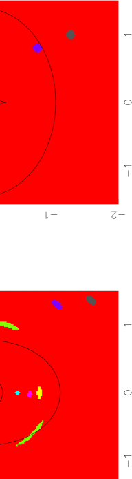
Figure 6.: Imaging of the source plane on the right through a simple lensing potential of the form $\Psi=\frac{1}{2}\ln(a^{2}+x^{2}+Qy^{2})$, corresponding to a flattened mass distribution with an inverse-cube radial density profile.

2.7. The mass-sheet degeneracy

Even though we can learn a lot from identifying multiple image pairs seen through a gravitational lens, it turns out to be impossible in principle to deduce the lensing potential completely from such data, no matter how detailed. The reason is that we do not have the luxury of being able to remove the lens and see the source plane undistorted. This unknown source plane propagates in the form of degeneracies in the lens model.

The most fundamental important degeneracy stems from the unknown scale of the source plane. If in the ray-trace equation 7 we scale the source location by a factor $k$, it is simple to construct a new lens which preserves all the image locations, as follows:

$$\beta=\theta-{D_{ds}\over D_{s}}\alpha(\theta)\quad\Rightarrow\quad k\beta=\theta-{D_{ds}\over D_{s}}\left[k\alpha(\theta)+{D_{s}\over D_{ds}}(1-k)\theta\right]\equiv\theta-{D_{ds}\over D_{s}}\overline{\alpha}(\theta).$$ (21)

Any source at location $\beta$ viewed through the lens with deflection angles $\alpha$ will be seen at the same location $\theta$ as a source at location $k\beta$ seen through the lens $\overline{\alpha}$. This new lens is obtained by rescaling the amplitude of the original lensing potential by a factor $k$, and adding a new quadratic lens potential

$$\Psi_{\rm sheet}={c^{2}\over 4}(1-k){D_{s}\over D_{d}D_{ds}}s^{2},$$ (22)

which corresponds to a sheet of constant surface mass density $\Sigma=(1-k)\Sigma_{\rm crit}$.

This mass sheet degeneracy can only be broken if (i) there is independent knowledge of the scale of the source plane, e.g., via source densities, (ii) sources at very different distances behind the lens are multiply imaged, so that the distance dependence of $\Sigma_{\rm crit}$ can be used to solve for $k$, or (iii) the lens model can be extended out to sufficiently large radii that a mass sheet can be ruled out on other grounds.

3. Strong lensing

Lenses in which $\kappa$ and $\gamma$ are of order 1 are termed strong. They produce multiple images, strong distortions, and very beautiful pictures of which a number can be found throughout this volume!

The two situations in which near-critical surface densities are attained are in the cores of massive galaxy clusters, and in the cores of galaxies (strictly speaking microlensing, described later, is also a form of strong lensing). Both galaxy and cluster lensing are discussed in detail in other contributions to this school.

Strong lenses are used in a number of applications: the main ones are non-dynamical mass measurements of galaxies and of clusters, determination of the Hubble constant, and studying distant galaxies with the aid of the lensing magnification.

3.1. Singular isothermal lens

A fiducial model for a galaxy or galaxy cluster lens is the pseudo-isothermal sphere,

$$\psi(r)=\sigma^{2}\ln\left(a^{2}+r^{2}\right).$$ (23)

It produces an asymptotically constant bending angle of

$$\alpha={4\pi\sigma^{2}\over c^{2}}{s\over\left(a^{2}+s^{2}\right)}^{1/2}\to 25\hbox{${}^{\prime\prime}$}\left(\sigma\over 1000\rm km\,s^{-1}\right)^{2}\quad\hbox{at large $s$}.$$ (24)

In this lens model, $\kappa$ and $(\gamma_{1}^{2}+\gamma_{2}^{2})^{1/2}$ are everywhere equal, and fall off as $s^{-1}$; on the critical line both are equal to $\frac{1}{2}$. The fact that the bending angle is constant outside the core means that all images are displaced radially outward by the same amount, and stretched tangentially along circles centered on the lens. The resulting arclets surrounding the lens are a generic feature of concentrated lenses, a manifestation of the lens’s outward ‘squeezing’ of the sky (Fig. 7). They are distinct from the giant arcs seen in elliptical lenses such as the one in Fig. 6: those are merging tangentially distorted image pairs.

Figure 7.: Arclet formation by a singular isothermal sphere lens: a circular source that is mapped outward by a constant deflection angle is tangentially stretched into an arclet.

3.2. The Hubble constant from time delays

If one ‘solves’ a lens system, this means that all angles between observer, lens and source have been defined. However there is no absolute distance scale that enters such a solution. The lens mass and the distances between lens, source and observer can be rescaled in proportion without any observable consequence to the images. However such a rescaling does scale the Fermat potential, and hence the time delay between images of the same source.

If a multiply-imaged source is variable, this offers the possibility to measure this time delay directly, and hence to set such a scale.

In practice this method suffers from some difficulties. The lens needs to be well-understood, which implies that either there is an independent measurement of its mass profile (including the environment of the lens itself)—the mass sheet degeneracy manifests itself here. The time delay needs to be unambiguously established, requiring long time series measurements, and feasible to monitor: this rules out cluster lenses where the delay runs into centuries. Also, the relative brightnesses of the images can be used as a further constraint on the model; however the magnification depends on higher derivatives of the potential and is therefore more sensitive to details. Furthermore, as discussed in §5 below, microlensing may affect the images in different ways which are unrelated to the large-scale lensing potential that determines the time delay.

The most robust systems for this work are four-image galaxy lenses. They provide a useful number of constraints on the lens, so that the potential may be sensibly constrained (although even here one quickly runs out of parameters!). They also yield a number of different time delay measurements, further tightening the model.

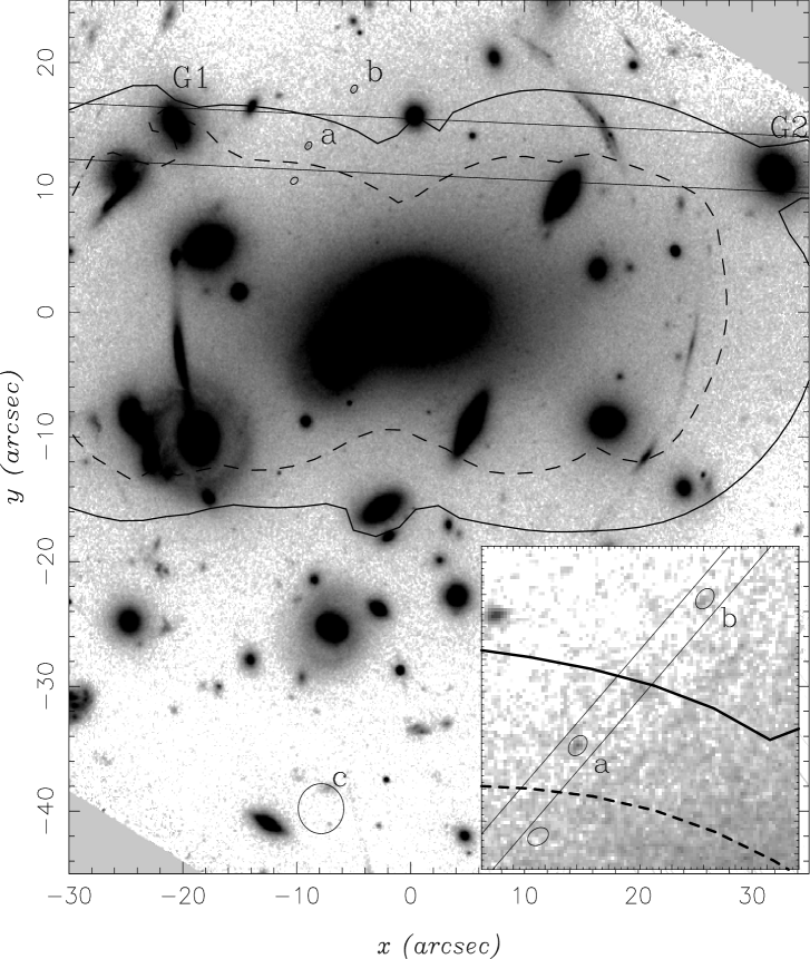
Figure 8.: The baby galaxy discovered behind Abell 2218. The source (a) was discovered in a systematic survey of the critical curve region (solid and dashed lines are the critical curves for source redshifts 5.5 and 1.1, respectively) in this cluster, and is a $z=5.5$ Ly-$\alpha$ emitter. Source (b) coincides with the predicted counterimage of this source for a redshift of 5.5. Both images have identical spectra. Had the source been at redshift 1.1, a second image would have been visible below the corresponding critical line (shown with the unlabelled ellipse).

3.3. Clusters as Gravitational Telescopes

Though their imaging properties are far from ideal, cluster lenses can provide a useful peek at distant galaxies, magnifying detail that is otherwise inaccessible. They also can boost faint sources into the realm of detectability.

A nice example is provided by the ’baby galaxy’ discovered behind Abell 2218 by Ellis et al. (2001). The cluster is one of the most well-understood ones, with a number of multiple image systems for which redshifts have been determined. By surveying the critical lines of this cluster, a $z=5.56$ source was discovered which is magnified a factor of 33 by the lens (Fig. 8). Even so, the source is barely visible on deep HST exposures! The spectrum shows a single emission line at 800nm, but no detectable continuum. Using the lens model, it was possible to predict where other images of the source should be visible as a function of the redshift of the source. When the line is identified with Ly-$\alpha$, such a second image was indeed seen, and it proved to have an identical spectrum. The gravitational telescope thus brought this tiny galaxy into view, and the lensing was also instrumental in securing the redshift of this source.

4. Weak Lensing

In weak lensing $\kappa,\gamma\ll 1$. There is no multiple image formation, only the slight distortion is under consideration in this regime. Weak lensing is nevertheless a very powerful tool, which is a result of two key facts: (i) it is possible to measure very small distortions; and (ii) there is a nice inversion possible between the observed distortion field and the lens mass distribution.

The details of these techniques are described in the review by Peter Schneider elsewhere in this volume; here we sketch the principles.

4.1. Measuring distortions

Figure 9.: An illustration of recovering the shear from a field of many randomy-oriented, elliptical galaxy images. On the left the galaxy images before (top) and after (bottom) applying a gravitational shear; on the right the corresponding distributions of image polarizations. In the unlensed case the polarizations cluster around zero, but a shear systematically moves the distribution.

If we were in the fortunate position that all galaxies were intrinsically round, then it would be simple to deduce the distortion matrix of the lens mapping: the circular images would be sheared into ellipses, and the size and direction of this shear would be easy to read off from the shape and orientation of the galaxies. This ideal can be approached by noting that while galaxies themselves come in many, basically elliptical shapes, they are randomly oriented. The average galaxy is thus round, in the sense that a stacking of a large number of galaxy images would give a round blob. If there is some distortion, this would affect all galaxy images equally, hence also the summed image. Consequently we should be able to measure the distortion from the way the blob is sheared.

In practice this is not the technique used to extract estimates of the lensing distortion, but it illustrates that the information is there. A different illustration of the same point is given in Fig. 9, where an ensemble of elliptical images is sheared, and the resulting systematic distortion uncovered by plotting the distribution of image polarizations

$$\left(\!\!\begin{array}[]{c}e_{1}\\ e_{2}\end{array}\!\!\right)={1\over I_{11}+I_{22}}\left(\!\!\begin{array}[]{c}I_{11}-I_{22}\\ 2I_{12}\end{array}\!\!\right)$$ (25)

where the $I_{ij}$ terms are different second moments $\int f(x_{1},x_{2})x_{i}x_{j}\,dx_{1}dx_{2}$ of each galaxy’s light distributions $f(x_{1},x_{2})$ in the image plane.

A delicate point in weak lensing is correction for all kinds of atmospheric and instrumental effects, which often produce considerably stronger distortions than the gravitational lensing. With existing techniques it is possible to derived reliable distortions with an accuracy of better than a few tenths of a percent. By obtaining distortion estimates in various bins on an image, a distortion map can be generated, which lays bare the effect of weak lensing by, for example, a cluster of galaxies. Also statistical studies in the field are now underway, in order to estimate the power spectrum of the gravitational lensing distortions, which can be related to the power spectrum of mass density fluctuations at intermediate redshifts.

4.2. Mass reconstruction

Once the distortion map has been made, the next step is to turn this into information about the gravitational lens. This is possile, because in the weak lensing regime, the distortion is a rather direct masure of the gravitational shear $\gamma_{i}$ of the lens (though one still needs to deal with the mass-sheet degeneracy, e.g. by setting the average mass density at a large distance to zero). Using eq. 19, it is simple to show that the shear components are related to $\kappa$, and hence the surface mass density distribution in the lens, via

$$\gamma_{1,1}+\gamma_{2,2}=\kappa_{1};\qquad\gamma_{2,1}-\gamma_{1,2}=\kappa_{2}.$$ (26)

These equations, which are in fact redundant, allow the measured shear field to be transformed into a $\kappa$ field, i.e., a picture of the lensing mass distribution. Different techniques exist to perform this inversion in practical situations, employing various kinds of regularization, and handling boundary conditions in different ways, but the principle is the same.

5. Microlensing

The final context in which gravitational lensing is encountered in modern astronomy is microlensing. Microlensing is done by compact lenses such as stars, and described by the point-lens formalism. An important difference with weak and strong lensing is that the multiple images produced by a microlens are usually not resolved, but only the combined (enhanced) flux of both images is seen. Because of this lack of resolution, microlensing can only be detected when the lens-observer-source alignment changes, since this alters the combined fluxes of the images. Detecting microlensing thus involves monitoring sources for brightness variations.

Figure 10.: The image configuration for point-mass lensing. The lens location is marked by the cross—this point is also the caustic for this lens. The corresponding critical curve (the Einstein circle) is shown as a dashed curve. Always two images are generated (the singularity breaks the odd-number-of-images rule), on either side of the lens. As the source tracks across the line of sight to the lens (open circles), the combined flux in both images (shown filled) rises and falls in a characteristic manner, as plotted in the top panel.

In quasars lensed by galaxies microlensing can occur as a result of the grainy gravitational potential of the lens galaxy. This is known as the high optical depth regime: microlensing in this context is not well described by lensing due to a single point mass.

In a more local setting, on the other hand, microlensing is very rare (for example, of order one star per million in the Galactic bulge or in the Magellanic Clouds is microlensed at any time), and studying the rates and characteristics of such microlensing events provides important information on the number and masses of compact objects along the line of sight.

The first surveys for microlensing were started in 1993, and the results as well as future prospects are reviewed in detail in Wyn Evans’ article in this volume.

6. Conclusions

Gravitational lensing has matured into a standard tool of astrophysics. It remains an attractive field because of the rather clean concepts employed, the very different insight it offers into mass determinations and geometrical measurements of the universe, the occasional peek it grants into the distant universe, and the often stunningly beautiful images one is forced to work with. As is well illustrated in the rest of this volume, there is plenty more life in lensing yet!

References

Schneider, P., Ehlers, J. & Falco, E.E. 1992, “Gravitational Lenses”, Springer.

Ellis, R.S., Santos, M.R., Kneib, J.-P. & Kuijken, K. 2001, ApJ, 560, L119