Chaos or Order in Double Barred Galaxies?

Abstract

Bars in galaxies are mainly supported by particles trapped around closed periodic orbits. These orbits respond to the bar’s forcing frequency only and lack free oscillations. We show that a similar situation takes place in double bars: particles get trapped around orbits which only respond to the forcing from the two bars and lack free oscillations. We find that writing the successive positions of a particle on such an orbit every time the bars align generates a closed curve, which we call a loop. Loops allow us to verify consistency of the potential. As maps of doubly periodic orbits, loops can be used to search the phase-space in double bars in order to determine the fraction occupied by ordered motions.

1 Introduction

Bars within bars appear to be a common phenomenon in galaxies. Recent surveys show that up to 30% of early-type barred galaxies contain nested bars erw+s02 . The relative orientation of the two bars is random, therefore it is likely that the bars rotate with different pattern speeds. Inner bars, like large bars, are made of relatively old stellar populations, since they remain distinct in near infrared wozn96 . Galaxies with two independently rotating bars do not conserve the Jacobi integral, and it is a complex dynamical task to explain how such systems are sustained. To account for their longevity, one has to find sets of particles that support the shape of the potential in which they move. Particle motion in a potential of double bars belongs to the general problem of motion in a pulsating potential l+g89 sridh88 , of which the restricted elliptical 3-body problem is the best known example. Families of closed periodic orbits have been found in this last problem, where the test particle moves in the potential of a binary star with components on elliptical orbits bro69 . However, such families are parameterized by values that also characterize the potential (i.e. ellipticity of the stellar orbit and the mass ratio of the stars), and their orbital periods are commensurate with the pulsation period of the potential. For a given potential, these families are reduced to single orbits separated in phase-space. The solution for double bars is formally identical, and there an orbit can close only when the orbital period is commensurate with the relative period of the bars. Such orbits are separated in phase-space, and therefore families of closed periodic orbits are unlikely to provide orbital support for nested bars. Another difficulty in supporting nested bars is caused by the piling up of resonances created by each bar, which leads to considerable chaotic zones. In order to minimize the number of chaotic zones, resonant coupling between the bars has been proposed sygnet88 , so that the resonance generated by one bar overlaps with that caused by the other bar.

Finding support for nested bars has been hampered by the fact that closed periodic orbits are scarce there. However, it is particles, not orbits, which create density distributions that support the potential. The concept of closed periodic orbit is too limiting in investigation of nested bars, and another description of particle motion, which does not have its limitations, is needed. Naturally, in systems with two forcing frequencies, double-periodic orbits play a fundamental role. Thus in double bars a large fraction of particle trajectories gets trapped around a class of double-periodic orbits. Although such orbits do not close in any reference frame, they can be conveniently mapped onto the loops m+s00 , which are an efficient descriptor of orbital structure in a pulsating potential. The loop is a closed curve that is made of particles moving in the potential of a doubly barred galaxy, and which pulsates with the relative period of the bars. Orbital support for nested bars can be provided by placing particles on the loops.

Here I give a systematic description of the loop approach, which recovers families of stable double-periodic orbits, and which can be applied to any pulsating potential. In §2 I use the epicyclic approximation to introduce the basic concepts, and in §3 I outline the general method.

2 The epicyclic solution for any number of bars

If a galaxy has a bar that rotates with a constant pattern speed, it is convenient to study particle orbits in the reference frame rotating with the bar. If two or more bars are present, and each rotates with its own pattern speed, there is no reference frame in which the potential remains unchanged. In order to point out formal similarities in solutions for one and many bars, I solve the linearized equations in the inertial frame. This is equivalent to the solution in any rotating frame, and the transformation is particularly simple: in the rotating frame the centrifugal and Coriolis terms are equivalent to the Doppler shift of the angular velocity. It is convenient to show it in cylindrical coordinates $(R,\varphi,z)$: if ${\bf e}_{z}$ is the rotation axis, then the $R$ and $\varphi$ components of the equation of motion for the rotating frame, $\ddot{\bf r}=-\nabla\Phi-2({\bf\Omega_{B}}\times\dot{\bf r})-{\bf\Omega_{B}}\times({\bf\Omega_{B}}\times{\bf r})$, can be written as

$$\ddot{R}-R(\dot{\varphi}+\Omega_{B})^{2} = -\frac{\partial\Phi}{\partial R},$$

$$R\ddot{\varphi}+2\dot{R}(\dot{\varphi}+\Omega_{B}) = -\frac{1}{R}\frac{\partial\Phi}{\partial\varphi}.$$

These equations are identical with the components of the equation of motion in the inertial frame,

$$\ddot{\bf r}=-\nabla\Phi,$$ (1)

where clearly the angular velocity $\dot{\varphi}$ in the rotating frame corresponds to $\dot{\varphi}+\Omega_{B}$ in the inertial frame. For the rest of this section I assume the inertial frame, in which the equation of motion (1) has the following $R$ and $\varphi$ components in cylindrical coordinates

$$\ddot{R}-R\dot{\varphi}^{2} = -\frac{\partial\Phi}{\partial R},$$ (2)

$$R\ddot{\varphi}+2\dot{R}\dot{\varphi} = -\frac{1}{R}\frac{\partial\Phi}{\partial\varphi}.$$ (3)

The $z$ component in any frame is $\ddot{z}=-\partial\Phi/\partial z$, but I consider here motions in the plane of the disc only, hence I neglect the dependence on $z$.

To linearize equations (2) and (3), one needs expansions of $R$, $\varphi$ and $\Phi$ to first order terms. The epicyclic approximation is valid for particles whose trajectories oscillate around circular orbits. For such particles one can write

$$R(t) = R_{0}+R_{I}(t),$$ (4)

$$\varphi(t) = \varphi_{00}+\Omega_{0}t+\varphi_{I}(t),$$ (5)

$$\Phi(R,\varphi,t) = \Phi_{0}(R)+\Phi_{I}(R,\varphi,t),$$ (6)

where terms with index $I$ are small to the first order, and second- and higher-order terms were neglected. The parameter $\varphi_{00}$ allows the particle to start from any position angle at time $t=0$, so that $\varphi_{0}=\varphi_{00}+\Omega_{0}t$. Asymmetry $\Phi_{I}$ in the potential is small and may be time-dependent. The angular velocity $\Omega_{0}$ on the circular orbit of radius $R_{0}$ relates to the potential $\Phi_{0}$ through the zeroth order of (2): $\Omega_{0}^{2}=(1/R_{0})(\partial\Phi_{0}/\partial R)\;|_{R_{0}}$. The zeroth order of (3) is identically equal to zero, and the first order corrections to (2) and (3) take respectively forms

$$\ddot{R_{I}}-4A\Omega_{0}R_{I}-2R_{0}\Omega_{0}\dot{\varphi_{I}} = -\frac{\partial\Phi_{I}}{\partial R}\;|_{R_{0},\varphi_{0}},$$ (7)

$$R_{0}\ddot{\varphi_{I}}+2\Omega_{0}\dot{R_{I}} = -\frac{1}{R_{0}}\frac{\partial\Phi_{I}}{\partial\varphi}\;|_{R_{0},\varphi_{0}},$$ (8)

where $A$ is the Oort constant defined by $4A\Omega_{0}=\Omega_{0}^{2}-\frac{\partial^{2}\Phi_{0}}{\partial R^{2}}|_{R_{0}}$.

We assume that the bars are point-symmetric with respect to the galaxy centre. Thus to first order the departure of the barred potential from axial symmetry can be described by a term $\cos(2\varphi)$. If multiple bars, indexed by $i$, rotate independently as solid bodies with angular velocities $\Omega_{i}$, the time-dependent first-order correction $\Phi_{I}$ to the potential can be written as

$$\Phi_{I}(R,\varphi,t)=\sum_{i}\Psi_{i}(R)\cos[2(\varphi-\Omega_{i}t)],$$ (9)

where the radial dependence $\Psi_{i}(R)$ has been separated from the angle dependence. No phase in the trigonometric functions above means that we define $t=0$ when all the bars are aligned. Derivatives of (9) enter right-hand sides of (7) and (8), which after introducing $\omega_{i}=2(\Omega_{0}-\Omega_{i})$ take the form

$$\ddot{R_{I}}-4A\Omega_{0}R_{I}-2R_{0}\Omega_{0}\dot{\varphi_{I}} = -\sum_{i}\frac{\partial\Psi_{i}}{\partial R}\;|_{R_{0}}\cos(\omega_{i}t+2\varphi_{00}),$$ (10)

$$R_{0}\ddot{\varphi_{I}}+2\Omega_{0}\dot{R_{I}} = \frac{2}{R_{0}}\sum_{i}\Psi_{i}(R_{0})\sin(\omega_{i}t+2\varphi_{00}).$$ (11)

In order to solve the set of equations (10,11), one can integrate (11) and get an expression for $R_{0}\dot{\varphi_{I}}$, which furthermore can be substituted to (10). This substitution eliminates $\varphi_{I}$, and one gets a single second order equation for $R_{I}$, which can be written schematically as

$$\ddot{R_{I}}+\kappa_{0}^{2}R_{I}=\sum_{i}A_{i}\cos(\omega_{i}t+2\varphi_{00})+C_{\varphi},$$ (12)

where $A_{i}=-\frac{4\Omega_{0}\Psi_{i}}{\omega_{i}R_{0}}-\frac{\partial\Psi_{i}}{\partial R}_{|R_{0}}$, $\kappa_{0}^{2}=4\Omega_{0}(\Omega_{0}-A)$, and $C_{\varphi}/2\Omega_{0}$ is the integration constant that appears after integrating (11). This is the equation of a harmonic oscillator with multiple forcing terms, whose solution is well known. It can be written as

$$R_{I}(t)=C_{1}\cos(\kappa_{0}t+\delta)+\sum_{i}M_{i}\cos(\omega_{i}t+2\varphi_{00})+C_{\varphi}/\kappa_{0}^{2}.$$ (13)

The first term of this solution corresponds to a free oscillation at the local epicyclic frequency $\kappa_{0}$, and $C_{1}$ is unconstrained. The terms under the sum describe oscillations resulting from the forcing terms in (9), and $M_{i}$ are functions of $A_{i}$. Hereafter I focus on solutions without free oscillations, thus I assume that $C_{1}=0$. These solutions will lead to closed periodic orbits and to loops. The formula for $\varphi_{I}(t)$ can be obtained by substituting (13) into the time-integrated (11). As a result, one gets

$$\dot{\varphi_{I}}=\sum_{i}N_{i}\cos(\omega_{i}t+2\varphi_{00})-\frac{2AC_{\varphi}}{\kappa_{0}^{2}R_{0}},$$ (14)

where again $N_{i}$ are determined by the coefficients of the equations above. Note that to the first order $\Omega_{0}[R_{0}+C_{\varphi}/\kappa_{0}^{2}]=\Omega_{0}[R_{0}]-2AC_{\varphi}/{\kappa_{0}^{2}R_{0}}$, thus the integration constants entering (13) and (14) correspond to a change in the guiding radius $R_{0}$, and to the appropriate change in the angular velocity $\Omega_{0}$. They all can be incorporated into $R_{0}$, and in effect the unique solutions for $R_{I}$ and $\varphi_{I}$ are

$$R_{I}(t) = \sum_{i}M_{i}\cos(\omega_{i}t+2\varphi_{00}),$$ (15)

$$\varphi_{I}(t) = \sum_{i}N^{\prime}_{i}\cos(\omega_{i}t+2\varphi_{00})+const,$$ (16)

where free oscillations have been neglected. The integration constant in (16) is an unconstrained parameter of the order of $\varphi_{I}$.

2.1 Closed periodic orbits in a single bar

In a potential with a single bar there is only one term in the sums (15) and (16), hereafter indexed with $B$. Consider the change in values of $R_{I}$ and $\varphi_{I}$ for a given particle after half of its period in the frame corotating with the bar. This interval is taken because the bar is bisymmetric, so its forcing is periodic with the period $\pi$ in angle. After replacing $t$ by $t+\pi/(\Omega_{0}-\Omega_{B})$ one gets

$$R_{I} = M_{B}\cos[\omega_{B}(t+\frac{\pi}{\Omega_{0}-\Omega_{B}})+2\varphi_{00}]$$

$$= M_{B}\cos(\omega_{B}t+2\pi+2\varphi_{00}).$$

Thus the solution for $R_{I}$ after time $\pi/(\Omega_{0}-\Omega_{B})$ returns its starting value, and the same holds true for $\varphi_{I}$. After twice that time, i.e. in a full period of this particle in the bar frame, the epicycle centre returns to its starting point and the orbit closes. Thus (15) and (16) describe closed periodic orbits in the linearized problem of a particle motion in a single bar.

2.2 Loops in double bars

When two independently rotating bars coexist in a galaxy (hereafter indexed by $B$ and $S$), there is no reference frame in which the potential is constant. Thus when a term from one bar in (15) and (16) returns to its starting value, the term from the other bar does not (unless the frequencies of the bars are commensurate). Therefore the particle’s trajectory does not close in any reference frame. However, consider the change in value of $R_{I}$ and $\varphi_{I}$ after time $\pi/(\Omega_{S}-\Omega_{B})$, which is the relative period of the bars. One gets

$$R_{I} = M_{B}\cos[\omega_{B}(t+\frac{\pi}{\Omega_{S}-\Omega_{B}})+2\varphi_{00}]+M_{S}\cos[\omega_{S}(t+\frac{\pi}{\Omega_{S}-\Omega_{B}})+2\varphi_{00}]$$

$$= M_{B}\cos(\omega_{B}t+2\pi\frac{\Omega_{0}-\Omega_{B}}{\Omega_{S}-\Omega_{B}}+2\varphi_{00})+M_{S}\cos(\omega_{S}t+2\pi\frac{\Omega_{0}-\Omega_{S}}{\Omega_{S}-\Omega_{B}}+2\varphi_{00})$$

$$= M_{B}\cos(\omega_{B}t+2\pi+2\varphi_{01})+M_{S}\cos(\omega_{S}t+2\varphi_{01}),$$

where $\varphi_{01}=\varphi_{00}+\pi\frac{\Omega_{0}-\Omega_{S}}{\Omega_{S}-\Omega_{B}}$. The same result can be obtained for $\varphi_{I}$. This means that the time transformation $t\rightarrow t+\pi/(\Omega_{S}-\Omega_{B})$ is equivalent to the change in the starting position angle of a particle from $\varphi_{00}$ to $\varphi_{01}$. Consider motion of a set of particles that have the same guiding radius $R_{0}$, but start at various position angles $\varphi_{00}$. This is a one-parameter set, therefore in the disc plane it is represented by a curve, and because of continuity of (15) and (16) this curve is closed. After time $\pi/(\Omega_{S}-\Omega_{B})$, a particle starting at angle $\varphi_{00}$ will take the place of the particle which started at $\varphi_{01}$, a particle starting at $\varphi_{01}$ will take the place of another particle from this curve and so on. The whole curve will regain its shape and position every $\pi/(\Omega_{S}-\Omega_{B})$ time interval, although positions of particles on the curve will shift. This curve is the epicyclic approximation to the loop: a curve made of particles moving in a given potential, such that the curve returns to its original shape and position periodically. In the case of two bars, the period is the relative period of the bars, and the loop is made out of particles having the same guiding radius $R_{0}$. Particles on the loop respond to the forcing from the two bars, but they lack any free oscillation. An example of a set of loops in a doubly barred galaxy in the epicyclic approximation can be seen in m+s97 . Since they occupy a significant part of the disc, one should anticipate large zones of ordered motions also in the general, non-linear solution for double bars.

3 Full nonlinear solution for loops in nested bars

Tools and concepts useful in the search for ordered motions in double bars are best introduced through the inspection of particle trajectories in such systems. For this inspection I chose the potential of Model 1 defined in m+s00 , where the small bar is 60% in size of the big bar, and pattern speeds of the bars are not commensurate. Consider a particle moving in this potential inside the corotation of the small bar. Simple experiments with various initial velocities show that if the initial velocity is small enough, the particle usually remains bound. A typical trajectory is shown in the left panels of Fig.1 – since it depends on the reference frame, it is written twice, for reference frame of each bar. Further experimenting with initial velocities shows that particle trajectories are often even tidier: they look like those in the right panels of Fig.1, as if the trajectories were trapped around some regular orbit.

Figure 1: Two example trajectories (one in the two left panels, one in the two right ones) of a particle that moves in the potential of two independently rotating bars. The particle is followed for 10 relative periods of the bars, and its trajectory is displayed in the frame corotating with the big bar (top panels), and the small bar (bottom panels). Each bar is outlined in its own reference frame by the dotted line. Large dot marks the starting point of the particle.

Fine adjustments of the initial velocity lead to a highly harmonious trajectory (Fig.2), which looks like a loop orbit in a potential of a single bar (see e.g. Fig.3.7a in bt87 ). This is only a formal similarity, but understanding it will let us find out what kind of orbit we see in Fig.2. The loop orbit in a single bar forms when a particle oscillates around a closed periodic orbit. Therefore two frequencies are involved: the frequency of the free oscillation, and the forcing frequency of the bar. On the other hand, the Fourier transform of the trajectory from Fig.2 shows two sharp peaks at frequencies equal to the forcing frequencies of the two bars (Fig.3). Thus the trajectory from Fig.2 also has two frequencies: this time these are the forcing frequencies from the two bars, while the free oscillation is absent. This is how the solution in the linear approximation (§2.2) was constructed. We conclude that in both the linear (epicyclic approximation) case and the general case we are dealing with doubly periodic orbits in an oscillating potential of a double bar, with frequencies equal to the forcing frequencies of the bars. In the epicyclic approximation, these orbits have a nice feature that particles following them populate loops: closed curves that return to their original shape and position at every alignment of the bars. One may therefore expect that also in the general case these particles gather on loops.

Figure 2: A doubly periodic orbit in the doubly barred potential, followed for 20 relative periods of the bars, and written in the frame corotating with the big bar (left), and the small bar (right). The long axis of each bar is marked by the dashed line. Dots mark positions of the particle at every alignment of the bars.

Figure 3: Fourier transforms of the trajectories from right panels of Fig.1 (dotted line) and from Fig.2 (solid line). The peaks in the solid line are related to the forcing frequencies of the bars, and the peaks in the dotted line are not.

If in the general case particles on doubly periodic orbits form a loop, one can construct it by writing positions of a particle on such an orbit every time the bars align. These positions are the initial conditions for particles forming the loop, because after every alignment, the $n^{th}$ particle generated in this way takes the position of particle $n+1$. The first 20 positions of a particle on a doubly periodic orbit are overplotted in Fig.2. They indeed seem to be arranged on a closed ellipse-like curve; the shape of this curve varies in time, but it returns to where it started at every alignment of the bars (Fig.4). This construction shows that in the general case particles on doubly periodic orbits also form loops. Note that positions of particles on other orbits, which involve free oscillations, when written at every alignment of the bars, densely populate some two-dimensional section of the plane, and do not gather on any curve. It is extremely useful for the investigation of the orbital structure in double bars that the appearance of the loop is frame-independent. Loops provide an efficient way to classify doubly periodic orbits, which has been hampered so far by the dependence of the last ones on the reference frame.

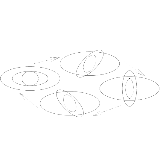
Figure 4: Evolution of the loop from Fig.2 during one relative period of the bars. The bars, outlined with solid lines, rotate counterclockwise. The loop is made out of points that represent separate particles on doubly periodic orbits.

It turns out that doubly periodic orbits play crucial role in providing orbital support for the pulsating potential of double bars. No closed periodic orbits have been proposed as candidates for the backbone of such a potential. If in a given potential of two bars there are loops that follow the inner bar, and other loops that follow the outer bar, then one may expect that such a potential is dynamically possible. An example of such a potential has been constructed in m+s00 . The loop from Fig.4 does not follow either bar in its motion, and therefore it is unlikely that it supports the assumed potential. It can be shown that in that potential, there are no loops which could support the two bars. Thus that potential is not self-consistent. This example shows how efficient is the loop approach in rejecting hypothetical doubly barred systems that have no orbital support.

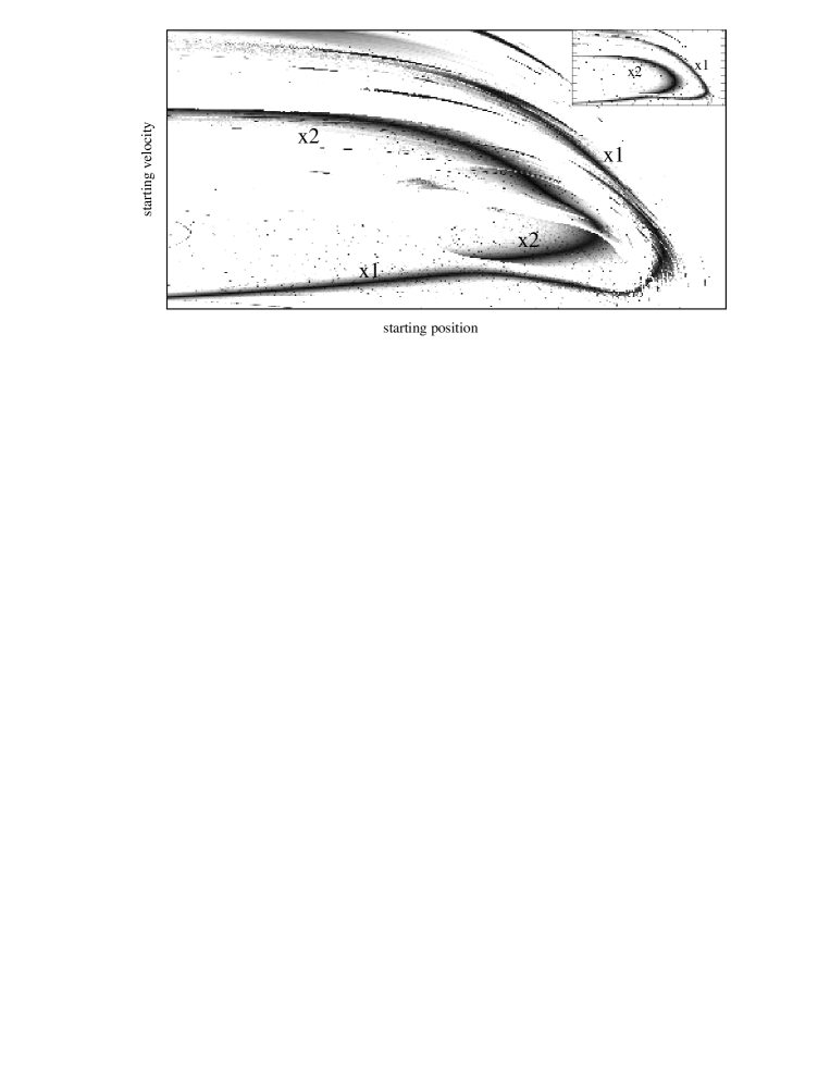
Figure 5: The width of the ring formed by particles trapped around loops in Model 2 from m+s00 as a function of the particle’s position along the minor axis of the aligned bars, and of its velocity (perpendicular to this axis). Darker color means smaller width. In the insert, the same is shown for rings around closed periodic orbits in a single bar (same model, but inner bar axisymmetric). Regions related to the $x_{1}$ and $x_{2}$ orbits, and to the loops originating from them, are marked.

Doubly periodic orbits in double bars are surrounded by regular orbits in the same way as are the closed periodic orbits in a single bar. In both cases, the trapped regular orbits oscillate around the parent orbit. The trajectory from the right panels of Fig.1 is an example of a regular orbit that is trapped around the doubly periodic orbit from Fig.2. How much of the phase space in double bars is occupied by orbits trapped around doubly periodic orbits? It can be examined by launching a particle from e.g. the minor axis of the bar, in the direction perpendicular to this axis, when the bars are aligned. If the particle is trapped, its positions at every alignment of the two bars lie within a ring containing the loop. The width of this ring depends on the particle’s position along the minor axis, and on its velocity. It is displayed in Fig.5 for the potential of Model 2 defined in m+s00 . Two stripes of low width appear on the diagram, which correspond to the $x_{1}$ and $x_{2}$ orbits in a single bar c+p80 (displayed in the insert). Thus in double bars there are doubly periodic orbits that correspond to closed periodic orbits in single bars. There are possible regions of chaos in double bars (white stripes in Fig.5), but overall loops in double bars and periodic orbits in single bars trap similar volumes of phase-space around them.

4 Conclusions

In a potential of two independently rotating bars, a large fraction of phase space can be occupied by trajectories trapped around parent regular orbits. These orbits are doubly periodic, with the two periods corresponding to the forcing frequencies of the two bars, but they do not close in any reference frame. Like particle trajectories oscillating around closed periodic orbits in a single bar, particle trajectories in double bars oscillate around the doubly periodic parent orbits. The structure of the parent regular orbits can be mapped using the loop approach, which allows us to single out dynamically possible double bars.

Acknowledgments. The concept of the loop as the organized form of motion in double bars benefits from the insight of Linda Sparke. I thank Lia Athanassoula for our collaboration that lead to this paper, and Peter Erwin for comments on the manuscript.

References

- (1) Binney, J. & Tremaine, S. 1987, Galactic Dynamics (Princeton: Princeton Univ. Press)
- (2) Broucke, R. A. 1969, Periodic Orbits in the Elliptic Restricted Three-Body Problem, Jet Propulsion Laboratory Report 32-1360
- (3) Contopoulos, G. & Papayannopoulos, Th. 1980, A&A, 92, 33
- (4) Erwin, P. & Sparke, L. S. 2002, AJ, 124, 65
- (5) Friedli, D., Wozniak, H., Rieke, M., Martinet, L., & Bratschi, P. 1996, A&AS, 118, 461
- (6) Louis, P. D. & Gerhard, O. E. 1988, MNRAS, 233, 337
- (7) Maciejewski, W. & Sparke, L. S. 1997, ApJL, 484, L117
- (8) Maciejewski, W. & Sparke, L. S. 2000, MNRAS, 313, 745
- (9) Sridhar, S. 1989, MNRAS, 238, 1159
- (10) Sygnet, J. F., Tagger, M., Athanassoula, E., & Pellat, R. 1988, MNRAS, 232, 733