Intrinsic Variability and Field Statistics for the Vela Pulsar: 2. Systematics and Single-Component Fits

Abstract

Individual pulses from pulsars have intensity-phase profiles that differ widely from pulse to pulse, from the average profile, and from phase to phase within a pulse. Widely accepted explanations do not exist for this variability or for the mechanism producing the radiation. The variability corresponds to the field statistics, particularly the distribution of wave field amplitudes, which are predicted by theories for wave growth in inhomogeneous media. This paper shows that the field statistics of the Vela pulsar (PSR B0833-45) are well-defined and vary as a function of pulse phase, evolving from Gaussian intensity statistics off-pulse to approximately power-law and then lognormal distributions near the pulse peak to approximately power-law and eventually Gaussian statistics off-pulse again. Detailed single-component fits confirm that the variability corresponds to lognormal statistics near the peak of the pulse profile and Gaussian intensity statistics off-pulse. The lognormal field statistics observed are consistent with the prediction of stochastic growth theory (SGT) for a purely linear system close to marginal stability. The simplest interpretations are that the pulsar’s variability is a direct manifestation of an SGT state and the emission mechanism is linear (either direct or indirect), with no evidence for nonlinear mechanisms like modulational instability and wave collapse which produce power-law field statistics. Stringent constraints are placed on nonlinear mechanisms: they must produce lognormal statistics when suitably ensemble-averaged. Field statistics are thus a powerful, potentially widely applicable tool for understanding variability and constraining mechanisms and source characteristics of coherent astrophysical and space emissions.

1 Introduction

Pulsars are believed to be highly magnetized neutron stars whose rotation causes highly nonthermal beams of radiation to be swept across the Earth. Most likely the radiation is produced over the magnetic polar caps of the star, which are offset from the rotational poles. The radiation’s high brightness temperatures require coherent emission processes such as plasma microinstabilities or nonlinear processes; however, despite many years of research, no agreement exists on which mechanisms dominate [Asseo 1996, Hankins 1996, Melrose 1996, Melrose & Gedalin 1999]. Proposed linear instabilities include: (i) Linear acceleration and maser curvature emission [Luo & Melrose 1995, Melrose 1996], in which electrons radiate coherently while accelerating in an oscillating large-scale field or on curved magnetic field lines, respectively. (ii) Relativistic plasma emission [Melrose 1996, Asseo 1996], in which a streaming instability either directly generates escaping radiation near harmonics of the electron plasma frequency $f_{pe}$ or else drives localized, non-escaping waves near $f_{pe}$ that are converted into escaping harmonic radiation by linear mode conversion or nonlinear processes. (iii) A streaming instability into a new, directly escaping mode (Gedalin, Gruman & Melrose 2002). Possible nonlinear mechanisms involve solitons, modulational instabilities, and strong turbulence wave collapse of intense localized wavepackets of waves driven near $f_{pe}$ (Pelletier, Sol, & Asseo 1988, Asseo, Pelletier, & Sol 1990, Asseo 1996, Weatherall 1997, 1998). Another possibility is an antenna mechanism, in which largescale low frequency wavepackets act as antennas for conversion of other higher frequency waves into radiation, due to acceleration of electrons in the combined wave fields (Pottelette, Treumann & Dubouloz 1999, Cairns & Robinson 2001). Standard analyses of linear and nonlinear growth rates suggest that numerous mechanisms are viable, in part due to uncertainties in the source plasma characteristics and location of emitting regions (e.g., above the polar cap or near the light cylinder). Accordingly new approaches are necessary.

Since the discovery of pulsars it has been known that only suitably long time averaging leads to a stable intensity profile. While this average profile is unique to each pulsar, individual pulses vary widely in intensity, often by a factor of 5 or more, from one phase to another in a given pulse and from one pulse to the next at a given phase. Illustrated in Figure 1 for Vela, this variability is intrinsic, clearly related to the emission mechanism and/or propagation effects, and has no accepted interpretation. This paper considers the variability in terms of its statistics, following Cairns, Johnston & Das (2001),hereafter called Paper I. In general, the variability includes phenomena known as drifting subpulses, microstructures, giant pulses, and giant micropulses. Subpulses are features that drift in time across the pulse window [Drake & Craft 1968, Manchester & Taylor 1977], while microstructures are concentrated features superposed on a subpulse that are sometimes quasiperiodic (Craft, Comella & Drake 1968, Kramer et al. 2002). Giant pulses [Cognard et al. 1996, Hankins 1996] and giant micropulses [Johnston et al. 2001] are very rare pulses with pulse-integrated fluxes $\stackrel{{\scriptstyle>}}{{\scriptstyle\sim}}10$ times the average.

Figure 1: Average flux profile as a function of phase bin for the Vela dataset (thick line), together with three superposed individual pulses (other lines). See Section 3 for more details.

Analyses of field statistics, such as the distributions of electric field strengths or intensities, are not yet standard in analyses of astrophysical radiation, in contrast to Fourier and correlation analyses related to propagation effects [Rickett 1977]. Probable reasons include (i) the strong theoretical motivations and benefits of considering field statistics were not clear before the advent of stochastic growth theory (SGT) (Robinson 1992, 1995, Robinson, Cairns & Gurnett 1993, Cairns, Robinson & Anderson 2000, Robinson & Cairns 2001, Cairns & Menietti 2001) and other theories such as self-organized criticality [SOC] (Bak, Tang & Weisenfeld 1987, Bak 1996), (ii) these motivations and benefits are not widely known in the astrophysical community, and (iii) high time resolution, coherently dedispersed data for high intensity sources, whose statistics are not strongly contaminated by instrumental/background noise, have only recently become available [Johnston et al. 2001, van Straten et al. 2001, Kramer et al. 2002]. Recent analyses of seven solar system wave phenomena show that all have well-defined field statistics that agree very well with the functional forms predicted by SGT, resolving longstanding theoretical problems pertaining to the burstyness, widely varying fields, and persistence of the waves (and driving particles) for unexpectedly large distances in the source. Giant pulses of some pulsars have power-law flux distributions [Cognard et al. 1996], as do giant micropulses [Johnston et al. 2001], potentially being interpretable in terms of SOC [Young & Kenny 1996], nonlinear modulational processes [Weatherall 1998, Paper I], or driven thermal waves [Cairns et al. 2000].

Pulsar variability and emission mechanisms can be addressed directly by analyzing the radiation statistics. Recently we presented a preliminary analysis of field statistics for the Vela pulsar [Paper I], demonstrating that the observed variability is intrinsic and corresponds to lognormal statistics at some pulsar phases, interpreting these statistics and the observed variability in terms of a pure SGT system, so that the associated pulsar emission mechanism involves only linear processes. The overall goal of the present paper and its companion (Cairns et al., 2002, hereafter called Paper III) is to present a detailed analysis of the Vela pulsar’s field statistics. Specific goals of this paper are: (i) to survey Vela’s field statistics as a function of phase, showing evolution from approximately Gaussian to power-law to lognormal to power-law to Gaussian distributions as the pulse phase varies from off-pulse to on-pulse to off-pulse again, (ii) present single-component Gaussian and lognormal fits to the field statistics for appropriate pulsar phases, (iii) demonstrate in detail that the variability corresponds to lognormal statistics near the peak of the pulse profile but Gaussian noise off-pulse, (iv) interpret the lognormal statistics in terms of SGT and linear emission mechanisms, and (v) discuss the results, including the constraints on nonlinear emission mechanisms. Paper III presents and interprets two-component fits to the observed field statistics over the remaining phase ranges; together these papers show that the Vela data are consistent with SGT applying, and with the emission mechanisms being purely linear, whenever the pulsar is detectable.

This paper proceeds by presenting required background information on theories for wave statistics (Section 2) and the Vela dataset (Section 3). Subsequently, the observed field statistics are surveyed, their evolution demonstrated, and initial analyses and associated interpretations described (Section 4). Detailed single-component fits to the observed field distributions for specific ranges of phase are then presented, first Gaussian intensity distributions off-pulse (Section 5) and then lognormal distributions near the center of the average pulse profile (Section 6). Brief descriptions of attempts to fit other distributions, specifically $\chi^{2}$ distributions and Gaussians in the field, to the data for these phase ranges are summarized in Section 7. Theoretical interpretations of these results are described and placed in context, first specifically for the Vela pulsar (Section 8) and then for other pulsars and astrophysical and solar system sources (Section 9). The conclusions are given in Section 10.

2 Theories for Wave Statistics

Wave growth in inhomogeneous plasmas naturally leads to bursty waves with widely varying fields. A qualitative rationale for this is as follows: (i) the plasma’s inhomogeneity leads to localized regions being favored for wave growth (e.g., the plasma instability depends upon plasma density, temperature etc.), (ii) the distribution function $f({\bf v})$ for the driving particles relaxes more in the growth sites (leading to larger wave fields there), (iii) this injects spatially and temporally varying fluctuations into $f({\bf v})$, (iv) these fluctuations cause burstyness and variable waves along the particle path, and (v) the system evolves to a statistically steady state where possible. These wave-particle interactions are expected to drive the system towards marginal stability, where wave emission and damping (and related energy inflows and outflows) are balanced, time- and volume-averaged. One likely condition for reaching a steady state is that the unstable features in $f({\bf v})$ be able to reform, at least partially; e.g., due to fast particles outrunning slow particles in a beam system [Robinson et al. 1993]. Different theories for wave growth are then characterized by different degrees of interaction between the waves, driving particles, and background plasma, leading to different wave statistics. Since these theories are not well known in the astrophysical literature, their salient features are summarized here in some detail.

SOC [Bak et al. 1987, Bak 1996] is relevant to systems with fully self-consistent interactions between the waves, driving particles and background plasmas and with no preferred distance or time scales. It predicts power-law statistics for the distribution of energy releases (e.g., wave energies), so that the distribution $P(I)$ of wave intensities $I$ obeys (where $I\propto E^{2}$ for the wave electric field $E$)

$$P(I)\propto I^{-\alpha}\ .$$ (1)

Typically the indices $\alpha$ approximately equal $1$, with a range $\approx 0.5-2$. Proposed examples include tokamak turbulence [Carreras et al. 1996] and solar flares [Lu & Hamilton 1991]. Also, Jovian “S” bursts have a power-law distribution for the radiation flux [Queinnec & Zarka 2001] and so may be an SOC system.

SGT (Robinson 1992, 1995l Robinson et al., 1993, Cairns et al. 2000, Robinson & Cairns 2001, Cairns & Menietti 2001) treats systems in which self-consistent wave-particle interactions occur in an independent, spatially inhomogeneous medium. The medium and wave-particle interactions then determine the relevant distance and time scales. In SGT the system evolves to a state in which (i) $f({\bf v})$ is close to time- and volume-averaged marginal stability but with fluctuations about this state which cause (ii) the wave gain $G$ to be stochastic variable. Relevant definitions are

$$E^{2}(t)=E_{0}^{2}e^{G(t)}\ ,$$ (2)

with $G=2\ln(E(t)/E_{0})$ for a reference field $E_{0}$, and

$$G(t)=\int_{-\infty}^{t}dt\ \gamma(t)$$ (3)

where $\gamma(t)$ is the (amplitude) growth rate of the waves. SGT is then a natural theory for bursty waves with widely varying fields (due to $\log E\propto G$ being a Gaussian random variable) that persist with the driving particles for unexpectedly large distances and/or times (due to the closeness to marginal stability). Moreover, SGT should be widely applicable since there is a natural qualitative route to an SGT state: writing the time integral in (3) as

$$\int_{-\infty}^{t}dt\ \gamma(t)={\LARGE\Sigma}_{i}\Delta G_{i}\ ,$$ (4)

then provided that sufficient fluctuations $\Delta G_{i}$ [associated with fluctuations in $f({\bf v})$] pass though a growth site during the characteristic time waves grow there, the Central Limit Theorem (CLT) predicts that $G$ will have Gaussian statistics irrespective of the detailed statistics of $\Delta G_{i}$. This means that $P(\log E)\propto P(G)$ obeys

$$P(\log E)=(\sqrt{2\pi}\sigma)^{-1}\ e^{-(\log E-\mu)^{2}/2\sigma^{2})}\ ,$$ (5)

where $\mu=\langle\log E\rangle$ and $\sigma$ are the average and standard deviation of $\log E$, respectively, and $\log\equiv\log_{10}$. That is, pure SGT predicts lognormal statistics for the field (Figure 2). In recent years pure SGT has been shown to be widely applicable (Robinson et al. 1993, Cairns and Robinson 1997, 1999, Cairns et al. 2000, Cairns & Grubits 2001, Cairns & Menietti 2001, Paper I).

Figure 2: Predictions for the $P(\log E)$ distribution for pure SGT (solid), SGT with a nonlinear decay process (dashed line), and SGT with wave collapse (dotted line).

SGT can coexist at moderate $E$ with nonlinear processes active at high $E$, causing characteristic modifications to the predicted lognormal statistics at fields close to and above the threshold field $E_{c}$ for the active nonlinear process. The presence or absence of active nonlinear processes can thus be constrained using field statistics, as used successfully in several applications. Two types of modification are known, as illustrated in Figure 2. First, when a three-wave decay process takes energy out of the measured waves, the $P(\log E)$ distribution is cutoff at $E\stackrel{{\scriptstyle>}}{{\scriptstyle\sim}}E_{c}$ with known analytic form [Robinson et al. 1993, Cairns & Menietti 2001, Cairns & Grubits 2001]. Second, the nonlinear process of wave collapse (Robinson 1997, Weatherall 1997, 1998), due to a self-focusing or modulational instability of a wavepacket, leads to a power-law tail at $E\stackrel{{\scriptstyle>}}{{\scriptstyle\sim}}E_{c}$. These indices are typically large: collapse of Langmuir waves in non-relativistic electron-proton plasmas leads to

$$P(E)\propto E^{-1}P(\log E)\propto E^{-\alpha}$$ (6)

with $\alpha$ varying between $4$ and $7$, depending on the dimensionality (2-D to 3-D) and shape (isotropic versus oblate versus prolate) of the wave packets and whether the collapse is subsonic or supersonic [Robinson & Newman 1990, Robinson 1997]. The characteristics of collapse, or even whether it occurs, are not so clear for the strongly magnetized and relativistic electron-positron plasmas relevant to pulsar magnetospheres: while a purely electrostatic analysis [Pelletier et al. 1988] suggests that solitons are stable to modulational instability and do not collapse, electromagnetic simulations suggest instead that the solitons are subject to modulational instability and do collapse (Weatherall 1997, 1998). Although the field statistics of these collapse events are not known, the qualitative behaviour is very similar to that for collapse in electron-proton simulations (Weatherall 1997, 1998). Accordingly, it is presumed hereafter that, if modulational instability occurs, then it leads to wave collapse and power-law field statistics described by (6) with indices similar to those given above for electron-proton simulations.

SGT also describes the statistics of waves driven by a linear instability from the thermal level $E_{th}$ [Robinson 1995, Cairns et al. 2000], being essentially a power-law with low index at fields $\stackrel{{\scriptstyle>}}{{\scriptstyle\sim}}E_{th}$, while thermal waves have a field distribution given by the product of a power-law with a Gaussian in $E^{2}$. In contrast, elementary burst theory [EBT] predicts exponential statistics (Melrose & Dulk 1982, Robinson, Smith & Winglee 1996) while the formerly standard theory for wave growth [Krall & Trivelpiece 1973, Melrose 1986], that of homogeneous exponential growth with constant growth rate until saturated at high fields by a nonlinear process or quasilinear relaxation (uniform secular growth), predicts $P(\log E)$ should be uniform (flat) below the nonlinear level [Robinson et al. 1993, Cairns & Robinson 1999]. While EBT appears consistent with solar microwave spike bursts [Robinson et al. 1996, Isliker & Benz 2001], the statistics of all systems published to date are inconsistent with uniform secular growth.

The final model considered here for field statistics and variability is that of Gaussian statistics in $I$, i.e.,

$$P(I)=(\sqrt{2\pi}\sigma_{I})^{-1}\ e^{-(I-I_{0})^{2}/2\sigma_{I}^{2}}\ ,$$ (7)

where $I_{0}=\langle I\rangle$ and $\sigma_{I}$ are the average and standard deviation of $I$. This is the standard expectation for background noise, for instance due to superposition of multiple random signals, so that the sky background, measurement noise, and sources with multiple unresolved sources should have $P(I)$ distributions with Gaussian statistics. Scattering of waves between the source and observer, due to refraction by density irregularities, can also lead to Gaussian $P(I)$, as sketched next. The Central Limit Theorem for a monochromatic (real, scalar transverse) field $E$ predicts Gaussian field statistics if sufficiently many ray paths contribute, whence the distribution $P(I)$ should then have an exponential distribution [Ratcliffe 1956, Rickett 1977], corresponding to a $\chi^{2}$ distribution with $2$ degrees of freedom. This distribution is well approximated by (7) if the scattering is weak and/or $\sigma_{I}\stackrel{{\scriptstyle<}}{{\scriptstyle\sim}}I_{0}$ [Ratcliffe 1956]. Intuitively, inclusion of finite bandwidth effects, due to multiple independent monochromatic signals contributing in a receiver bandwidth, should also lead towards Gaussian intensity statistics.

Relationships between the $P(I)$, $P(E)$ and $P(\log E)$ distributions follow from their normalization conditions, e.g., $\int dX\ P(X)=1$, and differentials. Accordingly

$$P(\log E)=\ln 10\ E\ P(E)=2\ln 10\ E^{2}\ P(I)\ ,$$ (8)

allowing (1), (5), and (6) to be related quickly. In summary, the field statistics predicted by the above theories are known and can be compared robustly with observational data to (i) determine the relevance of particular theories for wave growth, thereby constraining the physics of the wave growth and source region and the causes for the source’s variability, (ii) identify the presence or absence of nonlinear processes actively participating in the emission processes, and (iii) constrain the importance of scattering.

3 Dataset

The dataset consists of $20,085$ contiguous intensity pulses of the Vela pulsar, spanning approximately $30$ minutes, measured at $1413$ MHz by the Parkes radio telescope and described in detail elsewhere [Johnston et al. 2001]. Only a brief summary is given here. The measured quantities are the voltages (proportional to the received electric field strength) on two orthogonal feeds, which are frequency-downconverted, the DC offset removed with a time constant $\tau_{DC}$ long compared with the pulsar period ($\approx 88$ ms), and fed into a modified version of the Caltech and Princeton backend systems [Jenet et al. 1997, Stairs et al. 2000]. The backend system then samples the datastream in quadrature with 2-bit accuracy at 20 MHz and writes it to digital linear tape. Offline, dispersion effects are removed using coherent dedispersion techniques, the four Stokes parameters are recovered, instrumental polarization effects removed, and a flux calibrator (Hydra A) used to write the output data in terms of flux densities $F$ averaged over the backend’s 20 MHz bandwidth. The resulting dataset has $2048$ phase bins per pulse period, each of $\sim 44~{}\mu$s length, which is comparable to the scatter-broadening time at this frequency. About $1800$ 2-bit samples are thus used to calculate the flux in each phase bin every pulse. Arguments against this digitizing procedure significantly modifying the true field statistics are presented in section 9.

The resulting brightness temperature $T_{br}(\phi)$ at a given pulse phase $\phi$, proportional to $F$ and ideally to the antenna’s electric field squared, may be written as

$$T_{br}(\phi)=T_{rec}+T_{snr}+T_{back}+T_{psr}(\phi)\ ,$$ (9)

where $T_{rec}$ is the receiver (noise) temperature, $T_{snr}$ is the temperature of Vela’s supernova remnant, $T_{back}$ is the background temperature due to galactic synchrotron radiation, the Sun, and other sources, and $T_{psr}$ is the pulsar’s brightness temperature. Since the antenna points at the same location of the sky for the observing interval, removing the DC offset should eliminate $T_{snr}$ and $T_{back}$ from the final dataset (provided they do not vary on times $\ll\tau_{DC}$). Similarly, slow drifts in $T_{rec}$ will be removed, although rapid fluctuations corresponding to the receiver’s thermal noise persist and naturally dominate the observed field statistics at off-pulse phases (see Section 5 below).

While removal of the slowly-varying DC offset is an advantage in terms of observing weak sources above receiver and sky backgrounds, it is also a disadvantage for analyses of field statistics. There are at least three reasons. First, since $E^{2}\propto I\propto T_{psr}$, neglecting the time-steady, phase-averaged part of $T_{psr}$ ($\langle T_{psr}\rangle$) affects the field scale nonlinearly for fields $E$ such that $T_{br}(\phi)$ is within a factor of a few times $\langle T_{psr}\rangle$, thereby potentially modifying the field statistics there. Second, the logarithim function, which features prominently in SGT and the observed field statistics shown below, is undefined for negative fluxes (which occur in the dataset due to removal of the DC offset and due to thermal fluctuations in the receiver noise). Third, measurement of non-zero values of $\langle T_{psr}\rangle$ would permit more detailed investigation of the source physics, particularly if multiple wave populations are superposed, and perhaps allow competing physical models to be tested and distinguished. Possible origins for physically-significant, non-zero $\langle T_{psr}\rangle$ include synchrotron emission from the pulsar magnetosphere and coherently-produced radiation that undergoes scattering and diffusion as it propagates from its source, perhaps even changing the phase at which it is observed. Since the values $\langle T_{psr}\rangle$ are not available for these data, these issues are addressed by adding a constant offset flux

$$I_{off}^{\prime}=1250\ {\rm mJy}$$ (10)

to each sample in the dataset. Clearly, when fitting Gaussian intensity distributions (7) to the data, only relative variations in the centroid from $1250$ mJy are significant.

Comparisons between the data and Section 2’s theories are most easily accomplished by recasting the data in terms of fields and intensities. This is not inappropriate anyway, since the radiation fields incident on the antenna were first detected as voltages and the final calibrated fluxes are averaged over the detector’s $20$ MHz bandwidth. The calibrated intensity $I$ then equals the flux multiplied by the bandwidth and the field $E$ is proportional to $I^{1/2}$. Accordingly, rather than converting into SI units, the analyses below are cast in terms of variables $E^{\prime}$ and $I^{\prime}$, defined by

$$E^{\prime}= (F+1250{\rm mJy})^{1/2} \propto E\ ,$$ (11)

$$I^{\prime}= F+1250{\rm mJy} \propto I\ ,$$ (12)

which are related directly to the calibrated fluxes $F$ and whose units are in (mJy)^1/2 and mJy, respectively. Accordingly, $E^{\prime}$ and $I^{\prime}$ differ by multiplicative constants from $E$ and $I$ (and ideally to the incident field and intensity also), respectively, which correspond to constant scale factors or offsets along the abscissa axis in the linear and logarithmic plots of field statistics below.

Figure 1 shows the average pulse profile for relevant phase bins in mJy [Paper I], together with three superposed pulses that illustrate the variability. Note that the noise level is very low compared with many earlier analyses, allowing investigation of the intrinsic field statistics. Additionally, the pulses are sampled rapidly in time, reaching the limits imposed by scatter-broadening. This permits detailed investigation of the field statistics as a function of pulsar phase. The significant variations in field statistics with phase shown below suggest that rapid sampling is important if accurate analyses of field statistics is desired.

4 Identification of Regions

The off-pulse phase bins considered (phases $390-420$ and $600-630$, cf. Figure 1) have average intensities $I^{\prime}\approx I_{off}^{\prime}=1250$ mJy and maximum values $\approx 8000$ mJy. Only the on-pulse bins have $I^{\prime}\stackrel{{\scriptstyle>}}{{\scriptstyle\sim}}10^{4}$ Jy. Figure 3 surveys the whole dataset as a function of $\phi$: the top panel shows the maximum value of $\log E^{\prime}$ for each $\phi$, $\mu_{max}(\phi)$ (circles), and three averages for $\mu(\phi)=\langle\log E^{\prime}\rangle(\phi)$ (solid, dashed, and dotted lines), corresponding to averaging $\log E^{\prime}$ samples above specified intensity thresholds ($I^{\prime}\geq 10^{4}$, $2500$, and $0$ mJy, respectively). The Figure’s lower panel shows three estimates for $\sigma(\phi)$, which is the standard deviation of $\log E^{\prime}$, for these same phases and thresholds.

Figure 3: (Top) The maximum value of $\log E^{\prime}(\phi)$ (circles) and three estimates for the averages $\mu(\phi)=\langle\log E^{\prime}\rangle(\phi)$, calculated using three $I^{\prime}$ thresholds (solid – $10^{4}$ mJy, dashed – $2.5\times 10^{3}$ mJy, and dotted – 0 mJy), as functions of phase $\phi$ for the Vela dataset. (Bottom) Three estimates for $\sigma(\phi)$, using the line styles and intensity thresholds for (Top), as functions of phase.

The sharp, very localized peak in $\mu(\phi)$ and $\sigma(\phi)$ for a threshold of $10^{4}$ Jy at phases $429-433$, and its coincidence with the localized peak in $\mu_{max}$, demonstrates the appearance of a strongly phase-localized, intense component of the pulsar’s output. This corresponds to the giant micropulses identified previously [Johnston et al. 2001]. Otherwise Figure 3 shows smooth variations in $\mu$, $\mu_{max}$ and $\sigma$ with phase, including the “bump” identified for bins $550-600$ by Johnston et al. (2001). The effects of the different thresholds are not important for phases $\approx 460-540$, where the curves for the three thresholds agree well, corresponding to phases where $\mu(\phi)\stackrel{{\scriptstyle>}}{{\scriptstyle\sim}}0.5\log\sqrt{I_{off}}$ and the pulsar fields are typically well above the average value. However, the peaking of $\mu$ and $\mu_{max}$ at different phases ($\approx 480$ versus $\approx 450$) points towards different field statistics in these regions, as demonstrated in detail next, and to evolution in the number and characteristics of active components for the source.

Figure 4 shows the evolution of the field distribution $P(\log E^{\prime})$ as a function of pulsar phase. At each phase this distribution is calculated by binning the intensity time series in $\log E^{\prime}$ and normalizing so that $\int d(\log E^{\prime})P(\log E^{\prime})=1$. The $P(\log E^{\prime})$ distributions at phases $\stackrel{{\scriptstyle<}}{{\scriptstyle\sim}}428$ and $\stackrel{{\scriptstyle>}}{{\scriptstyle\sim}}600$ correspond to a Gaussian intensity distribution, being interpretable as Gaussian noise, as shown in detail in Section 5 below. However, for $\phi\stackrel{{\scriptstyle>}}{{\scriptstyle\sim}}429$ first a localized high-$I$ tail appears and disappears [the giant micropulses [Johnston et al. 2001]], after which an approximately power-law component appears at about phase $435$ and extends to increasingly high $E^{\prime}$ until about phase $455$. After this the entire distribution moves towards higher $E^{\prime}$, broadens, and the high-$E^{\prime}$ power-law slope becomes approximately parabolic in $\log P(\log E^{\prime})-\log E^{\prime}$ space at phase 465, corresponding to a lognormal distribution. The peak of this lognormal $P(\log E^{\prime})$ distribution continues to move to higher $E^{\prime}$ until about phase 480 but becomes narrower, corresponding to higher $\mu$ and smaller $\sigma$ in (5). Subsequently, the distributions continue to be approximately parabolic but move to lower $\mu$ and $\sigma$. Eventually the effects of Gaussian intensity noise become evident, giving rise to a non-parabolic tail at low $E^{\prime}$ for phases $\stackrel{{\scriptstyle>}}{{\scriptstyle\sim}}540$. In the phase range $\approx 545-600$ a power-law tail at high $E^{\prime}$ develops and then disappears, corresponding approximately to the “bump” [Johnston et al. 2001] in $\mu$ in Figure 3, after which the field distribution recovers the form in the off-pulse bins below phase $428$.

Figure 4 thus directly demonstrates that the Vela pulsar has different field statistics in neighboring ranges of phases; put another way, the field statistics vary with $\phi$ across the source. This immediately shows that field statistics can be used to probe the source physics.

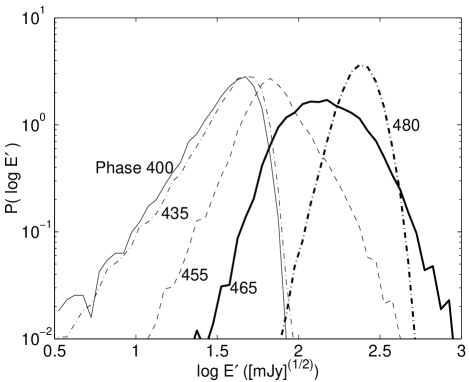
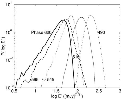
Figure 4: Distributions $P(\log E^{\prime})$ for chosen phases $\phi$, ranging from off-pulse ($\stackrel{{\scriptstyle<}}{{\scriptstyle\sim}}430$) to pulse-center (e.g., 470 and 490) to off-pulse again ($\stackrel{{\scriptstyle>}}{{\scriptstyle\sim}}600$).

The qualitative identifications given above are elaborated next by considering the quantities

$$R_{I}(\phi) = [I_{max}^{\prime}(\phi)-\langle I^{\prime}\rangle(\phi)]\ /\ \sigma_{I}(\phi)$$ (13)

$$R_{\mu}(\phi) = [\mu_{max}(\phi)-\mu(\phi)]\ /\ \sigma(\phi)\ ,$$ (14)

the first of which was considered previously, for example, by Johnston et al. (2001). A Gaussian intensity distribution at phase $\phi$ is expected to have $R_{I^{\prime}}(\phi)\stackrel{{\scriptstyle<}}{{\scriptstyle\sim}}5$, since almost all its samples should be within $\stackrel{{\scriptstyle<}}{{\scriptstyle\sim}}5\sigma_{I^{\prime}}(\phi)$ of the mean $\langle I^{\prime}\rangle(\phi)$. A similar statement follows for a lognormal field distribution, which should have $R_{\mu}(\phi)\stackrel{{\scriptstyle<}}{{\scriptstyle\sim}}5$. Figure 5 shows these quantities at different phases for the three intensity thresholds used in Figure 3. The $R_{I^{\prime}}(\phi)$ values in Figure 5’s top panel show that Vela’s field statistics are close to Gaussian in $I^{\prime}$ only for phases $\stackrel{{\scriptstyle<}}{{\scriptstyle\sim}}428$ and $\stackrel{{\scriptstyle>}}{{\scriptstyle\sim}}610$. The $R_{\mu}$ values in Figure 5’s bottom panel show that the field statistics are close to lognormal at phases $\stackrel{{\scriptstyle>}}{{\scriptstyle\sim}}460$ and $\stackrel{{\scriptstyle<}}{{\scriptstyle\sim}}540$, with particularly close agreement evident in the range $460-510$ where the traces for all three threshold are very close together.

Figure 5: The quantities $R_{I^{\prime}}$ and $R_{\mu}$ given by (13) and (14), respectively, are shown as functions of phase using the same intensity thresholds and line styles as Figure 3.

Figures 3 to 5 are thus all qualitatively consistent with the following identifications: phases $\stackrel{{\scriptstyle<}}{{\scriptstyle\sim}}428$ and $\stackrel{{\scriptstyle>}}{{\scriptstyle\sim}}600$ have Gaussian intensity statistics [Paper I], phases $429-433$ have non-Gaussian and non-lognormal statistics that correspond to giant micropulses [Johnston et al. 2001, Kramer et al. 2002], phases with $435-455$ and $545-600$ have an approximately power-law character at large $I^{\prime}$ and $\log E^{\prime}$; phases $460-540$ have lognormal field statistics (Papers I and III). These identifications are quantified next, using single-component fits, for the Gaussian-$I^{\prime}$ and lognormal regimes, refining and extending the analysis of Paper I. The approximately power-law domains are termed the “transition region” in Paper III, since these distributions are best interpreted in terms of vector convolution of a Gaussian and a lognormal component and not in terms of intrinsic power-law statistics. Two-component fits for the transition region and lognormal domains are detailed in Paper III.

5 Gaussian noise region

The field statistics at phases $\stackrel{{\scriptstyle<}}{{\scriptstyle\sim}}428$ and $\stackrel{{\scriptstyle>}}{{\scriptstyle\sim}}600$ are now shown in detail to be Gaussian in the intensity $I^{\prime}$, as expected for instrumental noise, background “noise” formed by incoherent superposition of a large number of small signals, and/or scattering. Figure 6 shows the $P(I^{\prime})$ distribution observed for phases $391-400$, calculated by binning the data into linear intensity bins and normalizing, together with the corresponding fit to (7), obtained using the Amoeba algorithm to minimize $\chi^{2}$ (Press et al. 1986). Restricting the fit to intensity bins with at least $100$ samples, the fit parameters are $\langle I^{\prime}\rangle=1220$ mJy (agreeing with $I_{off}^{\prime}$ to within less than the $100$ mJy bin width), $\sigma_{I^{\prime}}=1420$ mJy, $\chi^{2}=67$ for $N_{dof}=47$ degrees of freedom, and a significance probability $P(\chi^{2})=0.03$. Clearly the fit (7) agrees well with the observed data and has reasonable statistical significance.

Figure 6: Comparison of the observed intensity distribution $P(I^{\prime})$ for phases $391-399$ (circle symbols with error bars given by counting statistics) with the best fit to the prediction (7) for Gaussian statistics (solid line). Fits are performed where the dotted line shows that bins have $\geq 100$ counts and to the right of the vertical dashed line at $I^{\prime}=200$ mJy.

At high $I^{\prime}\stackrel{{\scriptstyle>}}{{\scriptstyle\sim}}7000$ mJy the observed distribution hints at deviations from the Gaussian form (7). The simplest explanation is that these high-$I^{\prime}$ samples correspond to pulsar emissions that slightly exceed the background. Put another way, the phase range 391-400 is not entirely off-pulse.

Lognormal fits to Figure 6’s data are clearly inferior (not shown). This is expected based on the strong dependence of the $R_{\mu}(\phi)$ curves in Figure 5 on the intensity thresholds used, in contrast to the lack of variation of the $R_{I^{\prime}}(\phi)$ curves on these thresholds. Thus these data are consistent with Gaussian intensity distributions and not lognormal field (or intensity) distributions. Analyses of other phases in the domain stated above yield similar fit parameters and statistics. This is expected on the basis of the very similar $P(\log E^{\prime})$ distributions shown in Figure 4.

6 Pure Lognormal Region

Single-component lognormal fits are presented in section 6.1 for the on-pulse phase domain $470-540$. Suggestions that a second component may also contribute are discussed in section 6.2. Two-component fits, which lead to very good agreement between observation and theory over the entire phase range, are presented in Paper III.

6.1 Single component fits

Figure 7 shows the $P(I^{\prime})$ distribution and its best Gaussian fit for phase 490, close to but after the peak in the pulsar’s average profile (Figure 1). The fit clearly fails at both low and high $I^{\prime}$, entirely missing the long tail at large $I^{\prime}$, and has $\chi^{2}=301$ for $N_{dof}=53$ and $P(\chi^{2})<10^{-36}$ for the fitted range of $I^{\prime}$ (dotted horizontal line). The variability at this phase is thus not described by Gaussian intensity statistics.

Figure 7: Comparison of the intensity distribution $P(I^{\prime})$ observed at phase 490 with the best fit (7) for Gaussian statistics (solid line). The circle symbols, error bars, dotted line, and vertical dashed line are as in Figure 6.

In contrast, Figure 8 shows that the $P(\log E^{\prime})$ distribution for phase 490 is well fitted by the pure SGT prediction (5): for bins with $\geq 100$ counts (dotted line) and $E^{\prime}\geq 10^{2}$ (mJy)${}^{1}/2$ ($I^{\prime}\geq 10^{4}$ mJy, which is $6\sigma_{I}$ above $\langle I^{\prime}\rangle$ in Figure 6), the fit parameters are $\mu=2.3$, $\sigma=0.096$, $\chi^{2}=27$ for $N_{dof}=19$ and $P(\chi^{2})=0.12$. Similarly the Kolmogorov-Smirnov test (Press et al. 1986) yields a significance probability of $0.47$. This fit is strongly statistically significant: pulsar variability at this phase is lognormally distributed and quantitatively consistent with the theoretical form (5) predicted for pure SGT. Note that the fit matches the data well even outside the fitted range of fields (vertical dashed line and horizontal dotted line), although the effects of the noise background become increasingly evident at fields $\leq 80$ (mJy)^1/2. It is worth emphasizing that the $P(I^{\prime})$ distribution in Figure 7 for $3\times 10^{4}\stackrel{{\scriptstyle<}}{{\scriptstyle\sim}}I^{\prime}\stackrel{{\scriptstyle<}}{{\scriptstyle\sim}}1.7\times 10^{5}$ mJy does not have an intrinsically power-law form but is instead best represented in terms of a lognormal form (Figure 8).

Figure 8: Comparison of the distribution $P(\log E)$ observed at phase 490 with the best fit (5) for lognormal statistics (solid line). The format is identical to Figure 6 except that the vertical dashed line is now at $E^{\prime}=100$ mJy^1/2.

Figure 9 presents the observed $P(\log E^{\prime})$ distribution and fit to the pure SGT prediction (5) for phase 510 . Again the observed distribution is well fitted by pure SGT with good statistical significance. For fields $E^{\prime}\geq 130$ (mJy)^1/2 the fit parameters are $\mu=2.1\pm 0.1$, $\sigma=0.10\pm 0.01$, $\chi^{2}=13$ for $N_{dof}=6$ with $P(\chi^{2})=0.04$. The statistical significance changes somewhat with the fitting threshold in $E^{\prime}$: requiring $E^{\prime}\geq 10^{2}$ (mJy)^1/2 yields $\mu=2.1\pm 0.1$, $\sigma=0.11\pm 0.1$, $\chi^{2}=42$, $N_{dof}=12$ and $P(\chi^{2})=3\times 10^{-5}$, while requiring $E^{\prime}\geq 150$ (mJy)^1/2 yields $\mu=2.1\pm 0.1$ and $\sigma=0.10\pm 0.01$ but $\chi^{2}=7$ for $N_{dof}=3$ and $P(\chi^{2})=0.07$. These varying statistical significances correspond to the varying contribution of the noise background to the observed distribution, due to the relatively weak pulsar fields at this phase and to $\mu$ approaching the background noise level. In each case the form of the distribution at high $\log E^{\prime}$ is very well fitted by the SGT prediction.

Figure 9: Comparison of the distribution $P(\log E^{\prime})$ observed at phase 510, in the same format as Figure 8, with the best fit to the prediction (5) for lognormal statistics (solid line).

Results similar to Figure 8 – 9 are found for phases $470-540$, although the statistical significance varies. Rather than showing more results for individual phases, Figure 10 shows the distribution $P(X)$ observed for phases $485-495$ [Paper I]. Here $X=[\log E^{\prime}-\mu(\phi)]/\sigma(\phi)$ is the field variable resulting from detrending variations in $\mu$ and $\phi$ with phase $\phi$. Comparison with (5) shows that purely linear SGT predicts the $P(X)$ distribution to be Gaussian with zero mean and unit standard deviation [Cairns & Robinson 1999]. Figure 10 demonstrates that the observations and SGT prediction agree well. The statistical significance is also good, with the Kolmogorov-Smirnov test yielding a significance probability of $0.1\%$.

Figure 10: Comparison of the distribution $P(X)$ for all data in phases 485–495 (plus signs), calculated using the procedure described in the text, with the pure SGT prediction (solid line).

One test of the results of Figures 8 – 10 is to compare the fits for $\mu$ and $\sigma$ with Figure 3’s values calculated directly from the data. Figure 11 shows that these values agree well, confirming that the fits are accurate and the lognormal component dominates the field statistics at these phases.

Figure 11: Comparison of $\mu$ and $\sigma$ (circle symbols) obtained by fitting the $P(\log E^{\prime})$ distributions to the SGT prediction (5) with the values obtained directly from the data set for $I^{\prime}\geq 2500$ mJy in Figure 3.

6.2 Initial evidence for a second component

Figures 8 – 10 show that the pure lognormal form (5) fits the data very well above the peak in the $P(\log E^{\prime})$ distribution but less well at low $E^{\prime}$. Specifically the observed distribution lies above the fit to (5) at low $E^{\prime}$, suggesting a contribution there from a second group (or component) of waves. This is not unexpected in view of the Gaussian statistics found at off-pulse phases (e.g., Figure 6), which if it corresponds to measurement noise, scattered radiation, or contributions from multiple unresolved, incoherently summed sources, might be expected to contribute at all phases.

In Paper III it is shown that the off-pulse Gaussian “noise” in Figure 6 indeed persists into the on-pulse bins and perhaps evolves into a second lognormal component. Performing two-component fits to the observed $P(\log E^{\prime})$ distributions then leads to very good agreement between observation and theory over almost the entire range of $E^{\prime}$ for all on-pulse bins. In particular, the approximately power-law $P(\log E^{\prime})$ distributions in Figure 4 correspond to vector convolution of the Gaussian component with an emerging lognormal component, while the clearly lognormal distributions observed at phases 460 – 540 are best modelled in terms of convolution of two lognormal components.

7 Attempts to Fit Other Distribution Functions

Attempts were made to assess the uniqueness of the Gaussian and lognormal fits presented heretofore, by also considering several other fitting functions: a Gaussian in the field (rather than the intensity), the SGT prediction for a thermal wave distribution [Robinson 1995, Cairns et al. 2000], and a $\chi^{2}$ distribution in $I^{\prime}$. Both the first and last of these are related to scattering theory [Ratcliffe 1956, Rickett 1977], the first being predicted for a scattered monochromatic real field and the latter (with $2$ degrees of freedom) for the intensity of a monochromatic scattered field. In more detail, a $\chi^{2}$ distribution with $n$ degrees of freedom corresponds to the distribution expected from summing a limited number $n$ of Gaussian-distributed variables and it is defined by

$$P_{\chi}(n,I^{\prime})=(I^{\prime}/I_{1})^{n/2-1}e^{-I^{\prime}/2I_{1}}/2^{n/2}\Gamma(n/2)\ .$$ (15)

Here $I_{1}$ is related to the average $\langle I^{\prime}\rangle$ by $I_{1}=\langle I^{\prime}\rangle/(n+2)$. In the limit $n\rightarrow\infty$ a $\chi^{2}$ distribution tends to a Gaussian.

Applying these three alternatives led to unsatisfactory results for all off-pulse phase bins (not shown), both in absolute terms and relative to the Gaussian intensity fits described in Section 5. This implies that the off-pulse data are best modelled in terms of Gaussian intensity statistics.

The results of these fits for on-pulse bins in the range $470-540$ were also unsatisfactory, both in absolute terms and relative to the lognormal fits in Section 6. Specifically: (i) These data were not well fitted as being Gaussian distributed in $E^{\prime}$ or as a thermal SGT distribution for any phase. (ii) Fits to the chi-squared distribution (15) invariably failed at high $\log E^{\prime}$ where the lognormal fits were clearly superior, due to an inability to fit the high-$I^{\prime}$ tail. (iii) While the data could be well fitted by (15) for some phase bins, but not all, the fit parameters $n$ and $I_{1}$ varied widely rapidly from phase bin to phase bin. (iv) Both the statistical significance of the fits and the size of the domains in $\log E^{\prime}$ for which good agreement existed between the $P(\log E^{\prime})$ data and fitting curves were generally considerably larger for the lognormal form (5) than for the chi-squared distribution (15). These statements are illustrated in Figure 12 for phase 490: for this phase (but not all) there is very good agreement at low $I^{\prime}$, as well as the typical inability to fit the high-$I^{\prime}$ tail. Moreover, the fit to (15) for phase 490 and bins with in excess of 100 samples has $n=12.3$, $I_{1}=3560$, $N_{dof}=54$, $\chi^{2}=93$ and $P(\chi^{2})=8\times 10^{-4}$, cf. the results in section 6, while the best fit for phase 510 has $n=8.3$, $I_{1}=1860$ mJy, and $P(\chi^{2})=0.02$. Accordingly, it is concluded that the on-pulse data are not well described in terms of Gaussian field statistics, thermal SGT, or a $\chi^{2}$ distribution in $I^{\prime}$, but are instead best described (for the four fitting functions attempted here) as lognormally distributed.

Figure 12: Comparison of the distribution $P(I^{\prime})$ observed at phase 490 with the best fit to prediction (15) for a chi-squared distribution, in the same format as Figure 6.

8 Theoretical Implications for the Vela Pulsar

In general, the observed field statistics are determined by intrinsic field statistics produced by relevant generation mechanisms, possible spatial variations across the source, and propagation effects. Propagation effects are discounted in the present context, since weak or moderate scattering of radiation by density fluctuations is typically predicted to cause Gaussian or exponential statistics of $I^{\prime}$ [Ratcliffe 1956, Rickett 1977], not lognormal statistics. In this dataset, then, Vela’s variability is not due to scattering by density irregularities. In general, though, scattering is expected to play some role in determining the field statistics of pulsars. The simplest interpretation is therefore adopted now, that the field statistics observed at each phase are intrinsic and are not significantly affected by spatial variations in the source. The possibility of two generation mechanisms being active at a given phase is deferred to Paper III.

For the phase range 470 - 540 considered above, where the Vela pulsar’s average pulse profile is well above the noise, the field distributions do not have power-law tails or nonlinear cutoffs but instead are consistent with lognormal statistics. Accordingly, these data are consistent with the observed variability being a direct manifestation of a simple SGT state, with no evidence for SOC or uniform secular growth. Put another way, Vela’s variability is due to lognormal field statistics and is consistent with the emission taking place in a source plasma that is in a simple SGT state.

The simplest interpretation is, then, that the absence of a power-law tail or cutoff in the $P(\log E^{\prime})$ distributions for these phases is inconsistent with nonlinear processes (e.g., Pelletier et al. 1988, Asseo et al. 1990, Asseo 1996, Weatherall 1997, 1998) such as wave collapse, modulational instability, and three-wave decay processes playing a significant role. Instead, the lognormal statistics observed are consistent with linear emission mechanisms, implying that a plasma instability in a SGT state either directly generates the radiation or else generates non-escaping waves that are transformed into escaping radiation by linear processes (e.g., mode conversion) alone. Moreover, these results are consistent with recent conclusions [Melrose & Gedalin 1999] that linear mechanisms are favoured on theoretical grounds and are made more topical by recent proposals of new linear emission mechanisms [Gedalin et al. 2002].

At a deeper level, however, nonlinear mechanisms cannot be ruled out entirely. Instead, stringent conditions are imposed: a nonlinear mechanism is viable only if it produces lognormal statistics when averaged over a suitable ensemble of nonlinear wavepackets or structures, with no evidence for a power-law tail or cutoff. Since existing simulations of collapse yield power-law statistics when ensemble-averaged in a homogeneous system [Robinson & Newman 1990, Robinson 1997], mechanisms involving collapse are not likely to be viable.

From the definitions of $\mu$ and $\sigma$ and the intensity decreasing with distance $R$ as $R^{-2}$, it is easy to show that $\sigma(R)$ is constant and that $\mu(R)=\mu(R_{0})-\log(R/R_{0})$, where $\mu(R_{0})$ is the value at the source’s edge ($R=R_{0}$). Taking the values $\mu=2.0$ and $\sigma=0.1$ to be representative of these phases, the distance $R=350$ pc for Vela, and the value $R_{0}=30$ m, yields $\mu(R_{0})\approx 20$. The value $R_{0}=30$ m results from assuming that the overall source is annular, with radius equal to the neutron star radius $\approx 10$ km, and dividing by the $2048$ phase bins used for Vela. Accordingly, the ratio $\mu_{0}/\sigma\approx 200$ in the source. The values $\mu_{0}$ and $\sigma$ will constrain future theoretical models for why SGT applies, similar to existing models for solar system phenomena [Robinson et al. 1993, Cairns & Robinson 1999, Cairns & Menietti 2001].

9 Discussion

The foregoing analyses are the first detailed applications of SGT to propagating EM radiation and, simultaneously, to extra-solar system sources (see also Paper I). Their success implies that radiation statistics are an underappreciated and potentially very powerful tool in astrophysics (and space physics), and suggests that SGT may well be widely applicable to coherent astrophysical sources. Of course, SGT is not likely applicable to all sources or indeed to all components of pulsar emissions, as discussed further in Paper III.

The importance of field statistics as a probe of source physics is shown above in terms of emission mechanisms. This is also shown empirically in terms of source structure by the demonstrated evolution in field statistics as a function of Vela’s phase, in particular by the field statistics ranging from Gaussian in $I$ off-pulse to approximately power-law, lognormal, and power-law on-pulse and to Gaussian in $I$ off-pulse again. This is the first detailed investigation of field statistics for a pulsar and the first demonstrated evolution in field statistics across a source. Quantitative discussion of how the fit parameters $\mu$, $\sigma$ etc. of the field statistics vary across Vela are deferred [Paper III], as is discussion of how representative the Vela results are to other pulsars.

It is appropriate to discuss the possibility that the intrinsic field statistics are modified by the digitization, summation, and coherent dedispersion procedures associated with the telescope backend system and consequent processing of the dataset (see section 3). Four observational results that argue against this possibility are the following: (i) the off-pulse statistics are Gaussian in $I^{\prime}$, as expected for receiver thermal noise; (ii) the on-pulse field statistics evolve smoothly with phase and the pulse profile (see section 4) and have well-defined functional forms; (iii) power-law field statistics are obtained from this dataset for Vela’s giant micropulses [Kramer et al. 2002] with indices of order those observed for giant pulses from other pulsars [Cognard et al. 1996, Johnston & Romani 2002, Romani & Johnston 2001, Cairns 2002]; (iv) the field distributions observed on-pulse can be fitted very well with lognormal functions [Paper I] and combinations of lognormal and Gaussian functions [Paper III], and can be interpreted theoretically in terms of existing theories for wave growth in plasmas; None of these results are expected a priori if measurement and analysis techniques have modified the intrinsic statistics significantly. Moreover, result (iii) is consistent either with the backend system and processing system not modifying the intrinsic field statistics or else with all analyses of giant pulses being similarly flawed. Thus, while modification of intrinsic field statistics by the measuring process is possible and must be kept in mind, the above points are strong arguments against Vela’s intrinsic field statistics being significantly modified for this dataset.

One final remark before concluding is that detailed analyses of field statistics would benefit from estimates for $\langle T_{psr}\rangle$ in (9), corresponding to the value $I_{off}^{\prime}$ in (10). This would allow an absolute scale for $E^{\prime}$ and $I^{\prime}$ to be estimated accurately and aid in interpreting detailed fits at low $E^{\prime}$ of the field statistics [Paper III].

10 Conclusions

Analysis of rapidly-sampled, coherently dedispersed data show for the first time that Vela pulsar’s variability corresponds to field statistics that are (i) well defined and (ii) evolve smoothly from Gaussian intensity statistics off-pulse to power-law and lognormal statistics on-pulse. Since theories for wave growth in inhomogeneous plasmas predict the field statistics, these observations allow the source plasma and emission physics to be probed. Detailed single-component fits to the observed field statistics confirm that the off-pulse variability corresponds to Gaussian intensity statistics, consistent with superposition of multiple incoherent signals and/or scattering, while the lognormal statistics observed near the peak of Vela pulsar’s average profile are consistent with the predictions of SGT for a purely linear system near marginal stability. The simplest interpretations are that the Vela pulsar’s on-pulse variability is a direct manifestation of an SGT state and that only linear emission mechanisms (either direct or indirect) are viable. This argues against some nonlinear theories for pulsar radio emissions. At a deeper level nonlinear mechanisms are not ruled out but are strongly constrained: viable mechanisms must produce lognormal statistics when suitably ensemble-averaged. Accordingly mechanisms involving wave collapse do not appear viable due to them yielding power-law statistics. The data suggest that scattering minimally affects the field statistics at on-pulse phases for Vela. Two-component fits for Vela’s power-law and lognormal domains, described elsewhere [Paper III], extend and strengthen these results, finding that the observed variability is consistent with lognormal statistics whenever the average pulse profile is above background.

These analyses of pulsar emissions represent the first applications of SGT to both non-solar-system sources and to propagating, free-space radio emissions. This generalizes the theory’s applicability significantly beyond the relatively localized, solar system, plasma waves considered previously. While SGT thus applies in all $8$ analyses performed by us to date, other field statistics are sometimes observed for other wave phenomena. Analysis of field statistics is thus a powerful tool for understanding source variability and constraining emission mechanisms and source characteristics. This new window into the source physics is likely to be widely useful for coherent astrophysical and solar system radio emissions, as already found for plasma waves in space.

References

- [Asseo 1996] Asseo E. 1996, in ASP Conf Ser. 105, Pulsars: Problems and Progress, ed. S. Johnston, M. A. Walker, & M. Bailes (San Francisco: ASP), 147
- [Asseo et al. 1990] Asseo E., Pelletier G., Sol H. 1990, MNRAS, 247, 529
- [Bak 1996] Bak P. 1996, How Nature Works. Copernicus, New York.
- [Bak et al. 1987] Bak P., Tang C., Wiesenfeld K., 1987, Phys. Rev. Lett., 59, 381
- [Cairns 2002] Cairns I.H., 2002, Astrophys. J., submitted
- [Cairns & Grubits 2001] Cairns I.H., Grubits K.A., 2001, Phys. Rev. E, 64, 056408
- [Cairns & Menietti 2001] Cairns I.H., Menietti, J.D., 2001, J. Geophys. Res., 106, 29,515
- [Cairns & Robinson 1997] Cairns I.H., Robinson P.A., 1997, Geophys. Res. Lett., 82, 3066
- [Cairns & Robinson 1999] Cairns I.H., Robinson P.A., 1999, Phys. Rev. Lett., 82, 3066
- [Cairns & Robinson 2001] Cairns I.H., Robinson P.A., 2001, in Radio Astronomy at Long Wavelengths, ed. R.G. Stone, J.-L. Bougeret, K. Weiler, and M. Goldstein, Geophysical Monograh 119, American Geophysical Union, 37
- [Cairns et al. 2000] Cairns I.H., Robinson P.A., Anderson R.R., 2000, Geophys. Res. Lett., 27, 61
- [Paper I] Cairns I.H., Johnston S., Das P., 2001, ApJ, 563, L65 (Paper I)
- [Paper III] Cairns I.H., Das P., Johnston S., and Robinson P. A., 2002a, MNRAS, submitted (Paper III)
- [Carreras et al. 1996] Carreras B.A., Newman D.E., Lynch V.E., Diamond P.H., 1996, Plasma Phys. Rep., 22, 740
- [Cognard et al. 1996] Cognard I., Shrauner J.A., Taylor J.H., and Thorsett S.E., 1996, ApJ, 457, L81
- [Craft et al. 1968] Craft H.D., Comella, J.M., Drake F.D., 1968, Nature, 218, 1122
- [Drake & Craft 1968] Drake F.D., Craft H.D., 1968, Nature, 220, 231
- [Gedalin et al. 2002] Gedalin M.E., Gruman E., Melrose D.B. 2002, MNRAS, submitted
- [Hankins 1996] Hankins T.H., 1996, in ASP Conf. Ser. 105, Pulsars: Problems and Progress, ed. S. Johnston, M.A. Walker, & M. Bailes (San Francisco: ASP), 197
- [Isliker & Benz 2001] Isliker H., Benz A.O., 2001, A.&A., 375, 1040
- [Jenet et al. 1997] Jenet, F.A., Cook, W.R., Prince, T.A., Unwin, S.C., 1997, PASP, 109, 707
- [Johnston & Romani 2002] Johnston S., Romani R., 2002, MNRAS, 332, 109
- [Johnston et al. 2001] Johnston S., van Straten W., Kramer M., Bailes M., 2001, ApJ, 549, L101
- [Krall & Trivelpiece 1973] Krall N.A., Trivelpiece A.W., 1973, Principles of Plasma Physics. McGraw-Hill, New York
- [Kramer et al. 2002] Kramer M., van Straten W., Johnston S., Bailes M., 2002, MNRAS, 334, 523
- [Kuznetsov et al. 1986] Kuznetsov, E.A., Rubenchik, A.M., and Zakharov, V.E., Phys. Rep., 142, 103
- [Lu & Hamilton 1991] Lu, E.T., and Hamilton, R.J., 1991, Astrophys. J., 380, L89
- [Luo & Melrose 1995] Luo Q., Melrose D.B., 1995, MNRAS, 276, 372
- [Manchester & Taylor 1977] Manchester R.N., Taylor J.H. 1977, Pulsars. Freeman, San Francisco
- [Melrose 1986] Melrose D.B., 1986, Instabilities in Space and Laboratory Plasmas. Cambridge, Cambridge.
- [Melrose 1996] Melrose D.B., 1996, in ASP Conf. Proc. 105, Pulsars: Problems and Progress, ed. S. Johnston, M. A. Walker, & M. Bailes et al. (San Francisco: ASP), 139
- [Melrose & Dulk 1982] Melrose D.B., Dulk, G.A. 1982, Astrophys. J., 259, 844
- [Melrose & Gedalin 1999] Melrose D.B., Gedalin M.E. 1999, ApJ, 521, 351
- [Pelletier et al. 1988] Pelletier, G. Sol, H., and Asseo, E. 1988, Phys. Rev. A, 38, 2552
- [Pottelette et al. 1992] Pottelette R., Treumann R.A., Dubouloz N., 1992, J. Geophys. Res., 97, 12,029
- [Press et al. 1986] Press W.H., Flannery B.P., Teukolsky S.A., Vetterling W.T., 1986 Numerical Recipes. Cambridge, New York.
- [Queinnec & Zarka 2001] Queinnec J., Zarka P., 2001, Plan. Space Sci., 49, 365
- [Ratcliffe 1956] Ratcliffe J.A., 1956, Rep. Prog. Phys., 19, 188
- [Rickett 1977] Rickett B.J., 1977, Ann. Rev. Astron. & Astrophys., 15, 471
- [Robinson 1992] Robinson P.A., 1992, Sol. Phys., 139, 147
- [Robinson 1995] Robinson P.A., 1992, Phys. Plasmas B, 2, 1466
- [Robinson 1997] Robinson P.A., 1997, Rev. Mod. Phys., 69, 507
- [Robinson & Cairns 2001] Robinson P.A., Cairns I.H., 2001, Phys. Plasmas, 8, 2394
- [Robinson & Newman 1990] Robinson P.A., Newman, D.L., 1990, Phys. Fluids, 2999
- [Robinson et al. 1993] Robinson P.A., Cairns I.H., Gurnett D.A., 1993, ApJ, 407, 790
- [Robinson et al. 1996] Robinson P.A., Smith, H.B., Winglee, R.M., 1996, Phys. Rev. Lett., 76, 3558
- [Romani & Johnston 2001] Romani R., Johnston S. 2001, Astrophys. J., 557, L93
- [Stairs et al. 2000] Stairs I.H., Splaver E.M., Thorsett S.E., Nice D.J., Taylor J.H. 2000, MNRAS, 314, 459
- [van Straten et al. 2001] van Straten W., Bailes M., Britton M., Kulkarni S.R., Anderson S.B., Manchester R.N, Sarkissian J., 2001, Nature, 412, 158
- [Weatherall 1997] Weatherall J.C., 1997, ApJ, 483, 402
- [Weatherall 1998] Weatherall J.C., 1998, ApJ, 506, 341
- [Young & Kenny 1996] Young M.D.T., Kenny B.G., 1996, in ASP Conf Ser. 105, Pulsars: Problems and Progress, ed. S. Johnston, M.A. Walker, & M. Bailes (San Francisco, ASP), 179