Constraints on a Universal IMF from UV to Near-IR Galaxy Luminosity Densities

Abstract

We obtain constraints on the slope of a universal stellar initial mass function (IMF) over a range of cosmic star-formation histories (SFH) using $z\approx 0.1$ luminosity densities in the range from 0.2 $\mu$m to 2.2 $\mu$m. The age-IMF degeneracy of integrated spectra of stellar populations can be broken for the Universe as a whole by using direct measurements of (relative) cosmic SFH from high-redshift observations. These have only marginal dependence on uncertainties in the IMF, whereas, fitting to local luminosity densities depends strongly on both cosmic SFH and the IMF. We fit to these measurements using population synthesis and find the best-fit IMF power-law slope to be $\Gamma=1.15\pm 0.2$ (assuming ${\rm d}N/{\rm d}\log m\,\propto\,m^{-\Gamma}$ for 0.5–120 M_⊙ and $m^{-0.5}$ for 0.1–0.5 M_⊙). This $M>0.5$ M_⊙ slope is in good agreement with the Salpeter IMF slope ($\Gamma=1.35$). A strong upper limit of $\Gamma<1.7$ is obtained which effectively rules out the Scalo IMF due to its too low fraction of high-mass stars. This upper limit is at the 99.7% confidence level if we assume a closed-box chemical evolution scenario and 95% if we assume constant solar metallicity. Fitting to the H$\alpha$ line luminosity density, we obtain a best-fit IMF slope in good agreement with that derived from broadband measurements.

Marginalizing over cosmic SFH and IMF slope, we obtain (95% conf. ranges): $\Omega_{\rm stars}$ = 1.1–2.0 $\times 10^{-3}$ $h^{-1}$ for the stellar mass density; $\rho_{\rm SFR}$ = 0.7–4.1 $\times 10^{-2}$ $h\,{\rm M}_{\odot}\,{\rm yr}^{-1}\,{\rm Mpc}^{-3}$ for the star-formation rate density, and; $\rho_{L}$ = 1.2–1.7 $\times 10^{35}$ $h\,{\rm W}\,{\rm Mpc}^{-3}$ for the bolometric, attenuated, stellar, luminosity density (0.09–5 $\mu$m). Comparing this total stellar emission with an estimate of the total dust emission implies a relatively modest average attenuation in the UV ($\lesssim 1$ magnitude at 0.2 $\mu$m).

1 Introduction

The luminosity density of the Universe in the range from about 0.2 $\mu$m to 2.2 $\mu$m, mid-UV to near-IR, is dominated by stellar emission. This wavelength range spans the peak in the spectra ($f_{\nu}$) of stars with effective temperatures from about 20000 K down to 2000 K. Therefore, measurements of the luminosity density in various broadbands across this range provide a powerful constraint on cosmic star-formation history (SFH) and/or a universal stellar initial mass function (IMF).

The stellar IMF describes the relative probability of stars of different masses forming (see Gilmore & Howell, 1998, for recent reviews and analyses). Its importance crosses many fields of astronomy from, for example, star formation (testing theoretical models) to cosmic chemical evolution (heavy metal production from high mass stars). It is widely used in the study of the SFH of galaxies from their integrated spectra. Generally, an IMF is assumed and used as an input to evolutionary, stellar population, synthesis models, and these models are fitted to integrated spectra.

The first calculation of an IMF was made by Salpeter (1955) based on the observed luminosity function of solar-neighborhood stars, converting to mass, correcting for main-sequence lifetimes and assuming that the star-formation rate (SFR) has been constant for the last 5 Gyr. Despite the uncertainties in mass-to-light ratios, stellar lifetimes and the SFR, this result (a power-law slope of $-1.35$ measured from about 0.3 to 15 M_⊙) is still commonly used today.

Measurements of the solar neighborhood IMF were reviewed by Scalo (1986) producing an IMF with a mass fraction peak around 0.5–1 M_⊙ (Fig. 1). When applied to galaxy populations, this IMF is unable to reproduce H$\alpha$ luminosities (Kennicutt, Tamblyn, & Congdon, 1994), and applied to cosmic evolution, is unable to match observed mean galaxy colors (Madau, Pozzetti, & Dickinson, 1998) due to a too low fraction of high-mass stars ($M>10$ M_⊙).

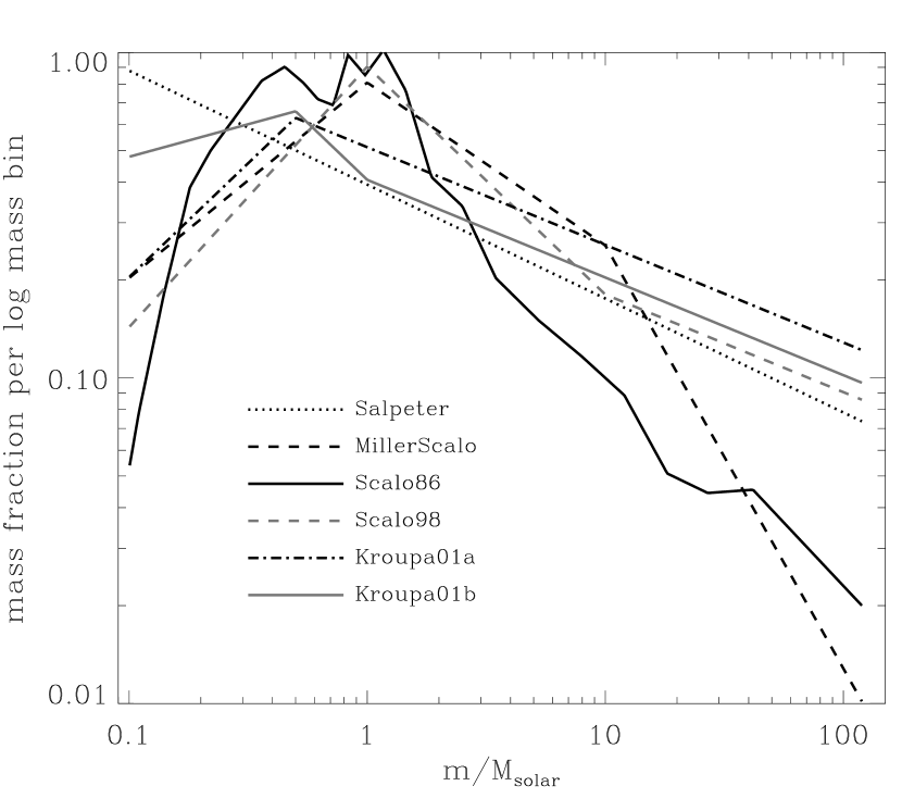
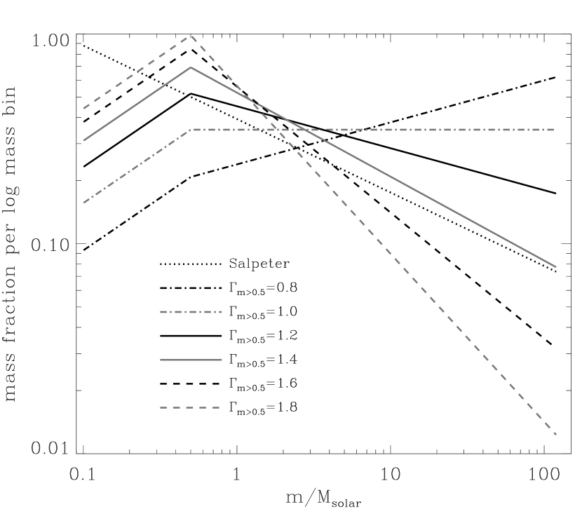
Figure 1: Stellar initial mass functions: mass fraction (per logarithmic mass bin) versus mass for the Salpeter (1955) IMF, the Miller & Scalo (1979) IMF, the Scalo (1986, 1998) IMFs, the Kroupa (2001, eqns. 2 and 6) IMFs (left panel) and the IMF parameterization of Equation 3 (right panel). All are assumed to be valid over the range 0.1–120 M_⊙. The integral of each curve is set to unity. Note that the slopes of the lines are equivalent to $1-\Gamma$ [$\,={\rm d}\log(m\,n_{\log m})\,/\,{\rm d}\log(m)$, see Eqn. 3 for definitions]. The $\Gamma$ values for $M>1$M_⊙ for the published IMFs are 1.35 (S55), 1.5/2.3 (MS79), $\sim$2.05/1.5 (S86), 1.7/1.3 (S98) and 1.3 (K01) (see also Table 2).

In a more recent review by Scalo (1998), he concluded that the field star IMF was of questionable use for a number of reasons (e.g. the derived IMF in the range 0.9–1.4 M_⊙ depends strongly on the assumed solar-neighborhood SFH). Instead, he summarized the results from studying star clusters in a triple-index power-law IMF as an estimate of an average IMF (Fig. 1). He also noted that “if the existing empirical estimates of the IMF are taken at face value, they present strong evidence for variations, and these variations do not seem to depend systematically on physical variables such as metallicity or stellar density”. The observed IMF variations from stellar counts could be largely due to statistical fluctuations and/or observational biases such as mass segregation within a star cluster (Elmegreen, 1999). These points, if correct, mean that the concept of a universal IMF is highly useful in the studies of integrated spectra of galaxies (since they are mostly the result of many star-formation regions and episodes) but the IMF is still uncertain at the level of 0.5 in the power-law slopes. By ‘universal IMF’, we mean an IMF that represents the average in a significant majority of galaxies and over a significant majority of cosmic time.

Measurements of the cosmic luminosity densities represent the $\lambda/\Delta\lambda\sim 6$ components of the “Cosmic Spectrum” which is the luminosity-weighted, average galaxy spectrum (Baldry et al., 2002). Thus, if there is a universal IMF, it should certainly apply to this spectrum and constraints on the IMF can be obtained by fitting population synthesis models. These constraints are degenerate with the assumed cosmic SFH. However, cosmic SFH is generally more accurately quantified than the SFH of any individual galaxy other than in the Local Group. For example, star-forming galaxies have been observed as far back as $z\sim 5$ (Dey et al., 1998), and there is evidence for reionization as early as $z\sim 20$ (Kogut et al., 2003), which for a Universe age of $13.7\pm 0.2$ Gyr (Spergel et al., 2003) gives a time of 12.3–13.7 Gyr since the onset of a significant rate of star formation in the Universe. The results for individual galaxies are often limited by age-metallicity degeneracy (Worthey, 1994) and recent bursts of star formation which can disguise their underlying age (Barbaro & Poggianti, 1997). Given our knowledge of cosmic SFH, we can then place constraints on a universal IMF by limiting the SFH we consider.

The primary knowledge of cosmic SFH comes from measuring the comoving density of SFR indicators at various redshifts (Madau et al., 1996). These SFR indicators include UV luminosities and emission-line luminosities that are dominated by light from short-lived high-mass stars. The conversion to SFR depends on the IMF. However, the relative cosmic SFH is well defined if the same indicator is used at each redshift regardless of the assumed IMF. Even if the indicator varies (e.g. 0.2 to 0.3 $\mu$m rest-frame UV), the derived cosmic SFH is less sensitive to the slope of the IMF than the local luminosity densities (0.2 to 2.2 $\mu$m). It is this principal that enables constraints on a universal IMF.

An analysis of this type was applied by Madau et al. (1998) using various luminosity densities (0.15 to 2.2 $\mu$m) spread over a range of redshifts (0–4). They fitted cosmic SFHs for three different IMFs. Here, we use a more quantitative approach to constraining a universal IMF slope and use more accurate, recent, local ($z\approx 0.1$) luminosity density measurements. Note that we assume that there is a universal IMF and do not constrain any variation in the IMF between different galaxies (see e.g. Wyse, 1997; Kroupa, 2002, for evidence for an invariant IMF). Even if there is some variation, the results presented here could be regarded as constraints on a luminosity-weighted, average IMF.

To summarize, if the cosmic SFH is assumed to be known, based on measurements of various SFR indicators with redshift, then local luminosity density measurements provide a constraint on a universal stellar IMF. The other principal factors to consider are chemical evolution (metallicity) and dust attenuation.

The plan of the paper is as follows. In Section 2, we describe details of recent luminosity density measurements. The measurements are illustrated in Figure 2 and summarized in Table 1. In Section 3, we describe our modeling and fitting procedure. A summary of the parameters used in the modeling is given in Section 3.5. In Sections 4 and 5, we present our results and conclusions.

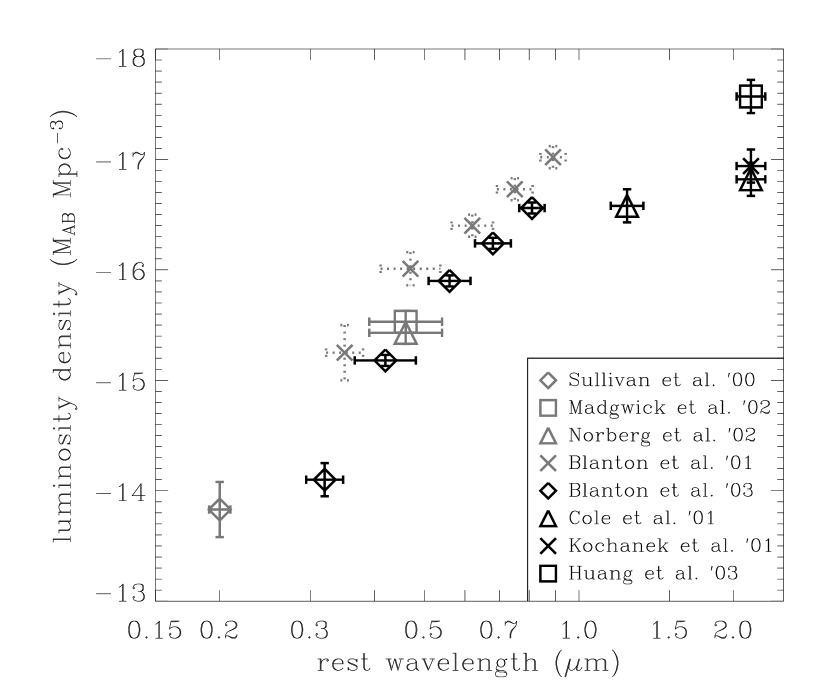
Figure 2: Local luminosity densities: absolute AB magnitudes per Mpc³ [$(h,\Omega_{m_{0}},\Omega_{\Lambda_{0}})$ = (1.0,0.3,0.7)] versus wavelength. The vertical bars represent uncertainties while the horizontal bars represent FWHM of the bandpasses. See Table 1 and Section 2 for details. We use the Sullivan et al. (2000), the Blanton et al. (2003b) and the $J$-$K$-band results for our fitting.

Table 1: Local luminosity densities from various surveys ($0<\bar{z}<0.2$)

band	reference	$\lambda_{\rm eff}$	$j+2.5\log h$	notes
		($\mu$m)	a(AB magnitudes)
bFOCA 0.2 $\mu$m	Sullivan et al. (2000)	0.20	$-13.83\pm 0.25$	$z\approx 0.15$, uncorrected for dust
cAPM $b_{\rm J}$	Madgwick et al. (2002)	0.46	$-15.53\pm 0.10$	$z\approx 0.10$
”	Norberg et al. (2002)	0.46	$-15.43\pm 0.10$	evolution corrections to $z=0.0$
dSDSS $u$	Blanton et al. (2001)	0.35	$-15.25\pm 0.25$	$z\approx 0.05$
SDSS $g$	”	0.47	$-16.01\pm 0.15$	$z\approx 0.10$
SDSS $r$	”	0.62	$-16.40\pm 0.10$	”
SDSS $i$	”	0.75	$-16.73\pm 0.10$	”
SDSS $z$	”	0.89	$-17.02\pm 0.10$	”
SDSS ${}^{0.1}u$	Blanton et al. (2003b)	0.32	$-14.10\pm 0.15$	evolution corrections to $z=0.1$
SDSS ${}^{0.1}g$	”	0.42	$-15.18\pm 0.05$	”
SDSS ${}^{0.1}r$	”	0.56	$-15.90\pm 0.05$	”
SDSS ${}^{0.1}i$	”	0.68	$-16.24\pm 0.05$	”
SDSS ${}^{0.1}z$	”	0.81	$-16.56\pm 0.05$	”
e2MASS $J$	Cole et al. (2001)	1.24	$-16.58\pm 0.15$	evolution corrections to $z=0.0$
2MASS $K_{s}$	”	2.16	$-16.82\pm 0.15$	evolution corrections to $z=0.0$
”	Kochanek et al. (2001)	2.16	$-16.94\pm 0.15$	$z\approx 0.03$
Hawaii $K_{s}$	Huang et al. (2003)	2.16	$-17.57\pm 0.15$	$z\approx 0.15$

^aluminosity density conversion: $j=-2.5\log(L_{\nu}/{\rm\,W\,Hz^{-1}\,Mpc^{-3}})+34.10$
^bFOCA magnitudes: assumed $m_{\rm AB}=m_{2000}+2.25$ (Milliard et al., 1992)
^cAPM magnitudes: assumed $m_{\rm AB}=b_{\rm J}-0.08$ (see Section 2.2)
^dSDSS magnitudes: assumed $m_{\rm AB}=(u,g,r,i,z)\,+\,(-0.04,0.035,0.015,0.015,0.00)$ (Blanton et al., 2003b)
^e2MASS, Hawaii magnitudes: assumed $m_{\rm AB}=J+0.9$, $m_{\rm AB}=K+1.8$ (Cutri et al., 2001)

2 Luminosity Density Measurements

In this section, we summarize the details of various luminosity density measurements and their conversion to AB magnitudes (Oke & Gunn, 1983) per comoving Mpc³. The zero point of the AB absolute magnitude scale is $4.345\times 10^{13}\>{\rm W}\>{\rm Hz}^{-1}$ (3631 Jy for apparent magnitudes). In general, an estimate of the total luminosity density from the galaxy population is obtained by an analytical integration of the Schechter (1976) function parameters, given by

$$j=M_{*}-2.5\log\left[\phi_{*}\,\Gamma_{\rm f}(\alpha+2)\right]+{\cal C}$$ (1)

where $\Gamma_{\rm f}$ is the gamma function and ${\cal C}$ represents corrections from the magnitude system defining the luminosity function to total AB magnitudes. The final luminosity densities are quoted for a cosmology where $(h,\Omega_{m_{0}},\Omega_{\Lambda_{0}})$ = (1.0,0.3,0.7) and $h=H_{0}/100\,{\rm km\,s^{-1}\,Mpc^{-1}}$. The surveys select redshifts to a limiting magnitude in the same wavelength as that of the luminosity density measurement.

2.1 Ultraviolet: 0.2 $\mu$m

An analysis of a mid-UV selected redshift survey is presented by Sullivan et al. (2000). The imaging for this survey covers about 6 deg² to a depth of about 21 AB magnitudes using the FOCA balloon-borne telescope (Milliard et al., 1992). The filter response approximates a Gaussian centered at 2015 Å with a full-width half maximum (FWHM) of 188 Å. The survey area covers four fields chosen with very low milky-way (MW) extinction [$E(B-V)\leq 0.015$]. Follow up spectroscopy was obtained using multi-object, optical spectrographs on the WIYN and WHT telescopes (Treyer et al., 1998).

Sullivan et al. measured the local luminosity density using a sample of about 200 galaxies ($0<z<0.4$) to estimate the luminosity function. The Schechter parameters without dust-correction were $(M_{*},\phi_{*},\alpha)=(-20.59,0.00955,-1.51)$. Integrating this function gives $-16.18$, and converting to AB magnitudes gives $-13.93$ using $m_{\rm AB}=m_{2000}+2.25$ (Milliard et al., 1992). We also correct the measurement to our default world model of $(\Omega_{m_{0}},\Omega_{\Lambda_{0}})$ = (0.3,0.7) from (1.0,0.0) assuming a redshift of 0.15. This gives a correction of about $+0.1$ magnitudes. The formal uncertainty from the fitting is 0.13 magnitudes. However, there are additional uncertainties: absolute calibration ($<0.25$ mags), MW extinction ($<0.15$ mags), conversion to total magnitudes ($<0.1$ mags), large-scale structure, incompleteness corrections, etc. We will assume an additional 1$\sigma$ uncertainty of 0.2 to be added in quadrature, so that $j=-13.83\pm 0.25$.

The limit of this survey is $m_{2000}=18.5$ which corresponds to $M_{*}$ galaxies at $z\approx 0.2$. With a steep faint-end slope of $-1.5$, the luminosity-weighted mean redshift is around 0.15 corresponding to the redshift position plotted by Sullivan et al. This is higher than our fiducial redshift of 0.10 (see below), giving a higher luminosity for any declining cosmic SFR at $z<0.5$. However, this may be counteracted by the lack of MW-extinction and total-magnitude corrections. For simplicity and since we do not want to assume a cosmic SFH and IMF, we will use the luminosity density as it was measured. Note that a couple of galaxies with obvious active galactic nuclei (AGN) characteristics were removed from their sample. We will assume the measured luminosity density does not have a strong, non-stellar, AGN component. Neither Sullivan et al. (2000) or Contini et al. (2002) found strong evidence for significant AGN contamination based on emission-line flux ratios.

2.2 Optical: 0.3 $\mu$m to 0.9 $\mu$m

The Sloan Digital Sky Survey (SDSS; York et al., 2000; Stoughton et al., 2002) has imaged over 2000 deg² in five bandpasses ($ugriz$) with effective wavelengths from 0.35 to 0.9 $\mu$m to a depth of about 21–22 AB magnitudes. Followup spectroscopy is also included as part of the SDSS for various targeting schemes, of which, the main galaxy sample (MGS; Strauss et al., 2002) is appropriate for determining cosmic luminosity densities. The MGS is a magnitude-limited galaxy sample ($r<17.77$) with a median redshift of 0.10. To form effectively complete samples in the other four bands, galaxies were selected to $(u,g,i,z)\>\lesssim\>(18.4,17.65,16.9,16.5)$.

The first luminosity densities from the MGS were published by Blanton et al. (2001). However, Wright (2001) found that these results overpredicted the near-IR luminosity density by a factor of 2.3 (compared to Cole et al., 2001; Kochanek et al., 2001). Since then, better analysis techniques, calibration and more data have allowed the optical luminosity density measurements to be significantly improved. We use the results of Blanton et al. (2003b) as the basis for our fitting here. One of their approaches was to $k$-correct and to evolve-correct to a fiducial redshift of 0.10. This reduces systematic uncertainties associated with these types of corrections because the median redshift of the SDSS is at this mark and the luminosity-weighted mean redshift is close to it. Thus, their results are most accurate for the shifted bandpasses, designated ${}^{0.1}u$, ${}^{0.1}g$, ${}^{0.1}r$, ${}^{0.1}i$ and ${}^{0.1}z$ (rest-frame bandpasses for galaxies at $z=0.1$). We use the ${}^{0.1}r$ band as the fiducial band and measure all colors with respect to it when comparing synthetic magnitudes with luminosity densities. We set a 1$\sigma$ uncertainty of 0.05 for the $g,r,i,z$ band measurements. This allows for some mis-calibration since the formal uncertainties of Blanton et al. are 0.03/0.02 for these bands. Using such small errors is appropriate since it is the relative ${}^{0.1}g,^{0.1}i,^{0.1}z$ to ${}^{0.1}r$ measurements that constrain the normalized SFH or IMF. In other words, the errors only need to represent the uncertainties in the colors and the absolute measurements of the luminosity densities need not be accurate to this level. An estimated conversion of SDSS to AB magnitudes is given and used by Blanton et al. (see also Table 1), and the magnitudes used by them are assumed to be close enough to total that a correction is not applied.

The new results of Blanton et al. (2003b) are in good agreement with $b_{\rm J}$ luminosity densities determined by Madgwick et al. (2002) and Norberg et al. (2002). These analyses were based on the Automated Plate Measuring (APM; Maddox et al., 1990) galaxy catalog with redshifts from the 2dF Galaxy Redshift Survey (2dFGRS; Colless et al., 2001). The conversion to AB magnitudes of $-0.08$ was based on an integration of the $b_{\rm J}$ curve (P. C. Hewett & S. J. Warren 1998 private communication) through a spectrum of Vega (Lejeune, Cuisinier, & Buser, 1997, computed by R. L. Kurucz). The $b_{\rm J}$ magnitudes were calibrated to total by comparison with deeper, CCD photometry.

2.3 Infrared: 1.0 $\mu$m to 2.5 $\mu$m

The Two Micron All Sky Survey (2MASS; Skrutskie et al., 1997) has imaged the whole sky in the $J$, $H$ and $K_{s}$ bands to a depth of 15–16 AB magnitudes (14.7, 13.9, 13.1 Vega mags, respectively). Cole et al. (2001) matched the second incremental data release to redshifts obtained by the 2dFGRS. With this data set, they determined the local $J$ and $K$ band luminosity functions. With $k$ and evolution corrections to $z=0$, the Schechter parameters were $(-22.36,0.0104,-0.93)$ and $(-23.44,0.0108,-0.96)$ for the $J$ and $K$ bands, respectively. Integrating these functions gives $-17.36$ and $-18.50$. The conversions to AB magnitudes are taken as $m_{\rm AB}=J+0.9$ and $K+1.8$ (Cutri et al., 2001) and the conversion to total magnitudes is estimated to be between $-0.08$ and $-0.15$ (we take $-0.12$). The uncertainties come from Poisson noise, the absolute calibration, the conversion to total magnitudes and large-scale structure. These are not all well defined but we will be conservative and use 0.15 for the 1$\sigma$ uncertainty so that $j=-16.58\pm 0.15$ and $j=-16.82\pm 0.15$ for the $J$ and $K$ bands, respectively.

The $K$-band luminosity function was also determined by Kochanek et al. (2001) using 2MASS imaging. Here, they determined the luminosity density using a shallower sample but with greater sky coverage for the redshifts. Their best estimate was obtained by summing separate luminosity functions for late and early-type galaxies: $(-22.98,0.0101,-0.87)$ and $(-23.53,0.0045,-0.92)$. The total luminosity density is then $-16.94$ in AB magnitudes after appropriate corrections (to AB, as above; to total, $-0.21$). This is in good agreement with the Cole et al. result.

A deeper $K$-band survey covering about 8 deg² was recently analysed by Huang et al. (2003). Imaging was taken with the University of Hawaii telescopes at Mauna Kea Observatory (Huang et al., 1997) with redshifts obtained using the 2dF facility on the AAT. The best-fit Schechter parameters were $(-23.70,0.0130,-1.37)$, giving a luminosity density of $j=-17.57$ after correcting to AB magnitudes. Even with a conservative error of 0.15, this result is $>3\sigma$ discrepant from the result of Cole et al. (2001). This discrepancy of 0.75 magnitudes is too large to be explained by cosmic evolution since the $K$-band luminosity density is dominated by the older stellar populations. Analysis by Huang et al. (2003) suggests it could be due to a local underdensity. We note that near-IR luminosity densities have larger uncertainties due to large-scale structure than bluer measurements. In underdense regions, the SFR per galaxy is higher (as noted by color-density and morphology-density relationships, e.g. Blanton et al., 2003a) which counteracts the effect on the UV luminosity density.

Given the above discrepancy in the near-IR luminosity densities, firstly, we will consider the Cole et al. results separately from the Huang et al. results in our fitting, and secondly, we will use an average $K$-band luminosity.

3 Modeling

We fit the data with synthetic magnitudes calculated using the PEGASE.2 evolutionary synthesis code (Fioc & Rocca-Volmerange, 1997, 1999) and integrating the spectra through the filter response curves (Fig. 3). The responses for the SDSS are taken from Stoughton et al. (2002), the FOCA filter curve is assumed to be Gaussian (Milliard et al., 1992) and the near-IR filter curves are taken from Cutri et al. (2001). We run the PEGASE models with nebular emission but ‘no extinction’ except we modified the code so that the absorption of Lyman continuum photons by dust was still included (following the prescriptions of Spitzer, 1978). This was done because our dust attenuation parameterization (Sec. 3.4) does not apply to this ‘pre-extinction’ of nebular continuum and line emission. The prescription for the models is described below including SFH, IMF and chemical evolution. We include further effects of dust attenuation on the output spectra.

Figure 3: FOCA, SDSS and 2MASS filters. The SDSS filters are shown ‘shifted’ to $z=0.1$ since we are fitting to the results of Blanton et al. (2003b). Each curve is normalized so that the integral of the normalized transmission $T\,{\rm d}\ln\lambda$ is equal to unity. Thus the height of each curve is related to its resolving power ($\lambda/\Delta\lambda$).

3.1 Cosmic SFH

For our modeling of cosmic star-formation history we use a ‘double power-law’ parameterization (Baldry et al., 2002):

$${\rm SFR}\>\propto\begin{array}[]{ll}(1+z)^{\beta}&\hbox{ for }0<z<1\\ (1+z)^{\alpha}&\hbox{ for }1<z<5\\ \end{array}$$ (2)

The SFRs from the two power-laws are the same at $z=1$ and star formation is started at $z=5$. Clearly, there are many other possible cosmic SFHs other than defined by these two parameters. However, the resulting synthetic spectra are highly degenerate with SFH. We chose this two-parameter model because the $\beta$ parameter provides a good match to direct measures of SFR at $z\lesssim 1$ and the $\alpha$ parameter allows us to add high-redshift star formation in a well-defined way. We assume a cosmology corresponding to $(h,\Omega_{m_{0}},\Omega_{\Lambda_{0}})$= (0.7,0.3,0.7). Most importantly this determines the timescale for cosmic SFH measurements.

Examples of this parameterized cosmic SFH are shown in Figure 4 with a timescale for the $h=0.7$ cosmology. Note that direct measures of the relative cosmic SFH with redshift do not depend on $H_{0}$. The Hubble constant changes the scaling factor at all redshifts by the same amount. However, our modeling of the cosmic SFH, to fit to local luminosity densities (fossil cosmology), does depend on $H_{0}$ because of the timescale dependence. The synthetic spectra are calculated at 11 Gyr corresponding to the fiducial redshift, $z=0.1$, with the chosen cosmology and $z_{\rm form}=5$.

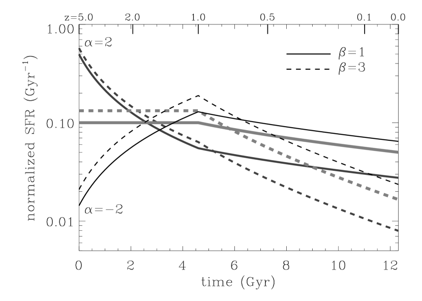
Figure 4: Examples of the parameterized cosmic SFH. The SFR is proportional to $(1+z)^{\beta}$ for $z<1$ and $(1+z)^{\alpha}$ for $1<z<5$. Each curve is normalized so that the total star formation between $z=5$ and $z=0$ is unity. The timescale is for $(h,\Omega_{m_{0}},\Omega_{\Lambda_{0}})$= (0.7,0.3,0.7). Six SFHs are shown with two values of $\beta$ (1,3) for each of three values of $\alpha$ ($-$2,0,2).

There is overwhelming evidence for a rise in SFR to $z=1$ from a variety of indicators (e.g. Haarsma et al., 2000; Hammer et al., 1997; Lilly et al., 1996; Rowan-Robinson et al., 1997). Recent estimates from compilations of measures of luminosity density with redshift out to $z=1$ give, for example, $\beta=2.7\pm 0.7$ (Hogg, 2002). If we take the formal 2$\sigma$ range from Hogg, we obtain a range of 1.3–4.1. However, some of the measurements compiled by him could be biased toward a steeper evolution (e.g. Lilly et al.) because of selection effects. Cowie, Songaila, & Barger (1999) found a shallower evolution of $\beta=1.5\pm 0.5$ based on rest-frame UV selection at all redshifts. To encompass the “evidence for a gradual decline” (Cowie et al.) to a steep decline (Lilly et al.), we will consider $\beta$ to be in the range 0.5–4.0.

High redshift ($z>1$) star formation is parameterized by $\alpha$ and $z_{\rm form}=5$. We do not try to exactly match high redshift measurements. The uncertainties are still large due to, for example, dust and surface brightness corrections. By taking $\alpha$ from $-2$ to $2$, we can approximate the effect of high-redshift star formation from a rapid decline at high redshift (Madau et al., 1996) to a flattening (Steidel et al., 1999) to a significant rise (Lanzetta et al., 2002). Note that the effect of any significant star formation in the $\sim$1 Gyr between $z=20$ and $z=5$ can be approximated by an increase in $\alpha$.

3.2 Universal IMF

Significant degeneracies exist with modeling the spectra of galaxies, e.g. age-metallicity. Given these uncertainties, modelers have generally assumed an IMF, typically the Salpeter (1955) IMF for modeling galaxy spectra. Here, we will assume a universal IMF (constant with time and environment) but we will consider different IMF power-law slopes. A double power-law IMF is chosen based on the rationale that there is a clear change in slope around 0.5 M_⊙ but no definitive change at higher masses (Kroupa, 2001). Our parameterization is

$$n_{\log m}\>\propto\begin{array}[]{ll}m^{-0.5}&\hbox{ for }0.1<m<0.5\\ m^{-\Gamma}&\hbox{ for }0.5<m<120\\ \end{array}$$ (3)

where $n_{\log m}\,{\rm d}\log m$ is the number of stars with logarithm of the mass in the range $\log m$ to $\log m+{\rm d}\log m$, $m$ is in units of solar masses with 0.1 M_⊙ and 120 M_⊙ being the IMF cutoffs. For the Salpeter (1955) IMF, $\Gamma=1.35$ in this formalism except, traditionally, the slope continues down to 0.1 M_⊙. A comparison between different IMFs is shown in Figure 1. Note that despite the average IMF of Scalo (1998) using a break at 1 and 10 M_⊙, figure 5 of that paper appears consistent with a single break at 0.5–0.8 M_⊙. Thus, as with Kroupa (2001), there is no strong evidence to rule out a double-power law IMF with a break at 0.5 M_⊙ being an adequate approximation of a universal IMF. For the low-mass slope, we use the average of the two Kroupa equations. We do not vary this slope since our results are less sensitive to this than the upper-mass slope.

3.3 Chemical evolution

For chemical evolution, we incorporate the closed-box evolutionary model within PEGASE which uses the models of Woosley & Weaver (1995) to estimate metallicity production via supernovae. The metallicity is controlled by a parameter $r$ (Baldry et al., 2002) that represents the total mass of stars formed between $z=5$ and $z=0$ divided by the total amount of gas initially available. Higher values of $r$ produce higher metallicity. The parameter can be greater than unity because of recycling of material. Since we are comparing different IMFs, we do not quote $r$ values but rather the value for the metallicity ($\bar{Z}$) averaged on the luminosity at $z=0.1$ (the $\bar{Z}$-$r$ dependence varies with IMF). Solar metallicity is considered to be $Z=0.02$ in the PEGASE models.

3.4 Dust attenuation

We wish to estimate the effective dust attenuation for the cosmic spectrum covering the UV to near-IR. However, we can not consider a standard slab or screen model as we would for an individual galaxy because the contributions to the luminosity densities come from many types of galaxies. Kochanek et al. (2001) estimated 54% and 46% contributions to the $K$-band from late- and early-type galaxies, respectively. The ratio is similar in the visible red bands from the SDSS survey though it depends on the chosen dividing line in color or morphology (Blanton et al., 2003a) . From Madgwick et al. (2002), 61% and 39% are the fractional contributions to the $b_{\rm J}$ band from late and early types, respectively, based on spectroscopic classification (assuming Types 2–4 for late, Type 1 for early). Late-type galaxies (Sa–Sd and starbursts) contribute about 90–95% of the light in the 0.2 $\mu$m UV (estimated from table 7 of Sullivan et al., 2000). This is consistent with the results obtained by Wolf et al. (2003) for the 0.28 $\mu$m UV at $z=0.3$, with $\sim 75/90$% contribution from late spectral types (3–4/2–4). Using the inclination-averaged attenuations of various galaxy types given by Calzetti (2001, table 3) and averaging over suitable distributions at each wavelength, we obtain cosmic spectrum attenuations in magnitudes of 1.1–1.35 at 0.15 $\mu$m, 0.4–0.55 at 0.45 $\mu$m, 0.2–0.3 at 0.8 $\mu$m and 0.05–0.1 at 2.2 $\mu$m.

To incorporate dust attenuation, we use a power law. The attenuation in magnitudes as a function of wavelength is approximated by

$$A_{\lambda}=A_{v}\left(\frac{\lambda}{\lambda_{v}}\right)^{-n}$$ (4)

where $A_{v}$ is the attenuation at the fiducial wavelength of $\lambda_{v}$. We use 0.56 $\mu$m since it matches the effective wavelength of our fiducial ${}^{0.1}r$ band and it is close to the standard $V$ band (0.55 $\mu$m).

If we fit to the cosmic spectrum attenuations, estimated above, we obtain $(A_{v},n)\approx(0.35,1.0)$ for our fiducial dust model. This curve is within the ranges in attenuation estimated above at each wavelength. Charlot & Fall (2000) found that for an average star-burst galaxy, $n$ was approximately 0.7 in a UV-to-visible attenuation law. Their model also included increased effective absorption in birth clouds which had a finite lifetime. Here, we assume that the the average of all galaxies (the luminosity densities considered here) can be approximated by a single effective optical depth. The average spectrum of the Universe is not that of a star-burst galaxy and the broadband colors are not strongly affected by emission lines. The luminosity density attenuations are naturally steeper than $n=0.7$ because of the increasing contribution of less dusty ellipticals as the wavelength is increased. Rather than restricting our fitting to a single value of $n$, we allow for a range from 0.8 to 1.2.

For $A_{v}$, we allow for a range from 0.2 to 0.55 magnitudes. For $n=1.0$, this is equivalent to a range in $A_{2000}$ from 0.55 to 1.55 magnitudes. This encompasses the difference between the uncorrected and dust-corrected luminosity densities of Sullivan et al. which amounts to 1.3 magnitudes. To avoid excessive attenuation at UV and near-IR wavelengths, we also set $0.5\leq A_{2000}\leq 1.6$ and $A_{K}\leq 0.15$ which reduces the $A_{v}$ range away from $n=1.0$. In general, we marginalize over attenuation, i.e., we chose the best fit parameters within the defined ranges that minimize $\chi^{2}$ when fitting the SFH and IMF.

3.5 Summary of parameters

In this section, we summarize the important parameters and ranges considered in our analysis and show the effect of varying some of the parameters.

• Synthetic spectra. PEGASE.2 (Fioc & Rocca-Volmerange, 1997, 1999): Padova tracks (Bressan et al., 1993), spectral libraries of Lejeune et al. (1997) and Clegg & Middlemass (1987). The Lejeune et al. library is principally derived from Kurucz (1992) model atmospheres. Nebular continuum and line emission is also included.

• Cosmology. $(h,\Omega_{m_{0}},\Omega_{\Lambda_{0}})$ = (0.7,0.3,0.7) (except luminosity densities are quoted for $h=1$, or, equivalently as $j+2.5\log h$). These values are fixed in our analysis.

• Cosmic SFH (Sec. 3.1, Eqn. 2). $\beta$ between [0.5,4.0], $\alpha$ between [$-$2,2], $z_{\rm form}=5$. Low-redshift ($z<1$) star formation is parameterized by ${\rm SFR}\propto(1+z)^{\beta}$ and high-redshift by $(1+z)^{\alpha}$.

• Universal IMF (Sec. 3.2, Eqn. 3). Power-law slopes of $-0.5$ (for $m<0.5$ M_⊙) and $-\Gamma$ between $[-0.8,-1.8]$ (for $m>0.5$ M_⊙) with $(m_{\rm min},m_{\rm max})$ = (0.1,120). The power-laws are with respect to $\log m$ so that the Salpeter IMF slope is $-1.35$.

• Chemical evolution (Sec. 3.3). Closed-box approximation with $\bar{Z}$ between [0.008,0.05] (Z_⊙=0.02) from $r$ between [0.1,1.4]. The final luminosity-weighted metallicity $\bar{Z}$ is principally a function of $r$ and the IMF.

• Dust attenuation (Sec. 3.4, Eqn. 4). Power-law slope of $-n$ between $[-0.8,-1.2]$ with $A_{v}$ between [0.2,0.55]. The ranges are also constrained by $0.5\leq A_{2000}\leq 1.6$ and $A_{K}\leq 0.15$.

Figure 5 shows the effects of varying one parameter on the synthetic spectra (normalized at the ${}^{0.1}r$ band) with respect to a model of $(\Gamma,\beta,\alpha,\bar{Z},A_{v},n)$ = (1.3, 2.5, 0, 0.018, 0.35, 1.0). Over our chosen parameter ranges, varying the IMF slope $\Gamma$ has the largest effect on the UV $-$ ${}^{0.1}r$ colors, with $\beta$ having the second largest effect. The metallicity has the largest effect on the near-IR $-$ ${}^{0.1}r$ colors.

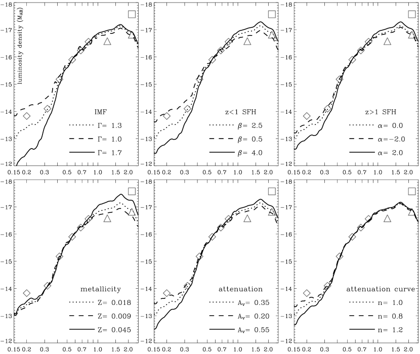
Figure 5: The effect of varying selected parameters individually: absolute magnitude versus wavelength. The lines represent synthetic spectra smoothed to $\lambda/\Delta\lambda\sim 10$. The dotted line is derived from the same set of parameters in every panel [$(\Gamma,\beta,\alpha,\bar{Z},A_{v},n)$ = (1.3, 2.5, 0, 0.018, 0.35, 1.0)]. All the spectra are normalized to $-15.90$ in the ${}^{0.1}r$ band filter (Blanton et al., 2003b). The symbols represent luminosity density measurements: the diamonds for Sullivan et al. and Blanton et al.; the triangles for Cole et al., and; the square for Huang et al.

4 Results

First, we fit to the UV-to-optical luminosity density measurements of Sullivan et al. (2000); Blanton et al. (2003b) with different near-IR measurements, considered separately: (a) using the Cole et al. (2001) $K$-band result (compilation designated SBC_K); (b) using the Huang et al. (2003) result (compilation SBH), and; (c) using the Cole et al. $J$-band result (compilation SBC_J) and not including the $z$-band measurement which is included in the first two compilations. Examples of fitted spectra are shown in Figure 6. This shows that the near-IR luminosity density measurements can be fitted, primarily by varying metallicity, while the UV-to-optical spectrum remains approximately the same. Within the range of metallicity considered here (0.4 Z_⊙–2.5 Z_⊙), the best fit is obtained to the SBC_K data. Here, all the measurements are within about $1\sigma$ of the synthetic magnitudes. The new results of Blanton et al. (2003b) and this analysis resolves the major discrepancy noted by Wright (2001) between the optical and near-IR luminosity densities. However, there is a significant discrepancy between the Hawaii and the 2MASS $K$-band luminosity densities and a discrepancy between the $J$-band result and the $z$-band/$K$-band results.

Figure 6: Example fits to data from SBC_K (UV, $ugriz$ and $K$ triangle; solid line), SBH (UV, $ugriz$ and $K$ square; dashed line) and SBC_J (UV, $ugri$ and $J$; dotted line). The lines represent the fitted synthetic spectra smoothed to $\lambda/\Delta\lambda\sim 10$. The parameters for these fits were $(\Gamma,\beta,\alpha,\bar{Z},A_{v},n)$ = (1.1, 4.0, 0, 0.022, 0.20, 0.9) for SBC_K, (1.1, 3.5, 0, 0.048, 0.44, 0.8) for SBH and (1.1, 4.0, 0, 0.009, 0.22, 0.8) for SBC_J. See text for details.

Neither of the infrared surveys is ideal for comparison with the SDSS survey results. The 2MASS survey is too shallow (median $z\sim 0.05$ at the limit of the extended source catalog) for direct comparison with the $z=0.1$ analysis and the Hawaii survey goes deeper but has a significantly smaller area (8 deg²). Note that the Sullivan et al. result only uses about 200 galaxies but it is consistent with the ${}^{0.1}u$ band result. Improved surveys are needed to resolve the near-IR luminosity density discrepancies and to reduce the uncertainties in UV luminosity densities.

We first look at constraints on the metallicity and IMF for a given cosmic SFH (marginalizing over dust attenuation). We compute $\chi^{2}$ and determine the confidence levels of $\Delta\chi^{2}$ = (1.0, 2.3, 6.2, 11.8) corresponding to (68.3%) 1-parameter and (68.3%, 95.4%, 99.73%) 2-parameter confidence limits. The resulting contours are shown in Figure 7 for a cosmic SFH with $\beta=2.5$ and $\alpha=0$ (Hogg, 2002; Steidel et al., 1999). As expected, the best fit metallicity is dependent on the near-IR data: the SBC_K data has a best fit metallicity around 1–1.5 Z_⊙; SBH data, $>2$ Z_⊙, and; SBC_J data, $<1$ Z_⊙. The SBC_K set of data is in agreement with solar neighborhood measurements of the metallicity which give an average close to solar (Haywood, 2001). The SBH data is in disagreement with solar metallicity at the 99.7% confidence level.

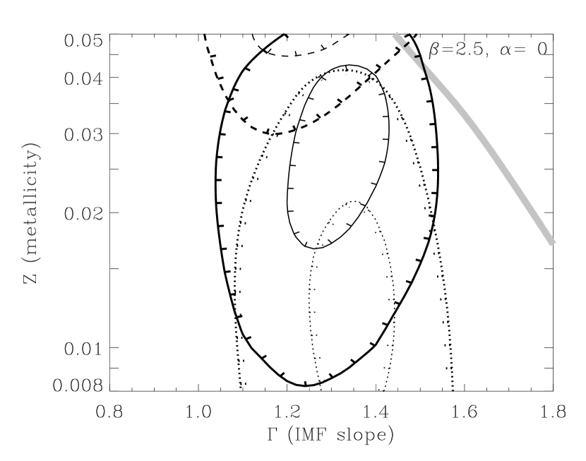
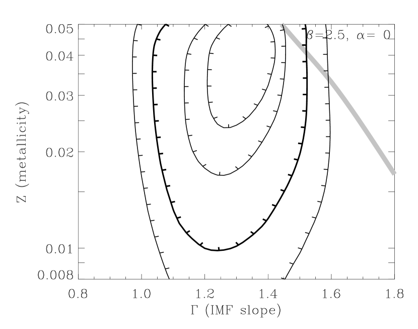
Figure 7: Joint confidence levels over metallicity and IMF slope assuming a cosmic SFH ($\beta=2.5$, $\alpha=0$). Left: The contours represent confidence levels for the SBC_K data (solid lines), SBH data (dashed lines) and SBC_J data (dotted lines). The levels correspond to 68% 1-para. and 95% 2-para. confidence limits, marginalized over dust attenuation. The thick gray line represents the approximate upper limit on the luminosity-weighted $\bar{Z}$ due to chemical evolution (from the closed-box model of PEGASE). Any $\chi^{2}$ values above this line are linearly extrapolated. Right: The same except the confidence limits are for the SBav data which uses an average near-IR luminosity estimate (Eqn. 5), and the levels represent the 68% 1-para. and 68%, 95%, 99.7% 2-para. confidence limits.

For the rest of the paper, we use an average estimate of the $K$-band luminosity corresponding to

$$j=-16.88\pm 0.25$$ (5)

from Cole et al. (2001) and Kochanek et al. (2001). The uncertainty was increased, and the $J$-band was not included, so that the constraints on the IMF were not dependent on the discrepancies noted above. This 1$\sigma$ range in the $K$-band luminosity density is also similar to the range determined by Bell et al. (2003). The metallicity-IMF contours for this data set (compilation designated SBav) are also shown in Figure 7. The best fit IMF slope, $\Gamma=1.3\pm 0.1$, shows the tightness of the constraint if the SFH is known. The best-fit metallicity is greater than solar but for other cosmic SFHs (e.g. $\beta=2.5$ and $\alpha=2$), the best fit is around solar. In general, there is minimal degeneracy between $\Gamma$ and metallicity for the data, i.e. the choice of metallicity does not significantly affect the constraints on the IMF slope.

Note that there is an upper limit on the metallicity as a function of $\Gamma$ due to the closed-box model (Fig. 7). Insufficient metals can be produced in the available time to raise the average metallicity above a certain limit and this limit decreases as the fraction of high-mass stars in the IMF decreases. This chemical evolution limit is derived from the PEGASE code using the upper yields of Woosley & Weaver (1995).

The pattern shown in Figure 7 is similar as $\beta$ is varied except the best-fit $\Gamma$ shifts. To illustrate this, we now fix $\bar{Z}$ equal to 0.02 for the SBav fit and show joint confidence levels in $\beta$ versus $\Gamma$ in Figure 8. We plot the result for three values of $\alpha$. All the plots show a broad degeneracy with a slope of $-7\pm 1$. In other words, the best-fit $\Gamma$ decreases by about $-0.14$ for each $+1$ increase in $\beta$. Note that the metallicity was chosen to be consistent with the solar neighborhood and so that the closed-box model was valid out to $\Gamma$ of 1.8 with only minimal extrapolation (see Fig. 7).

Figure 8: Joint confidence levels over $\beta$/$\alpha$ and IMF slope for three different values of $\alpha$ ($-$2,0,2) / one value of $\beta$ (2.5) and for a chemical evolution closed-box approximation with $\bar{Z}=0.02$. The contours represent 68% 1-para. and 68%, 95%, 99.7% 2-para. confidence levels for the SBav data, marginalized over dust attenuation.

The choice of high redshift star formation (defined by $\alpha$) makes little difference on the best-fit $\Gamma$ (Fig. 8). Marginalizing over SFH ($\beta$ & $\alpha$), we obtain a best fit for $\Gamma$ in the range 0.85–1.3 (68% conf.) and a strong upper limit of $\Gamma<1.7$ (99.7% conf.). This is our principal result. In other words, assuming a declining SFR from $z=1$ to the present day ($\beta\geq 0.5$) then the present luminosity densities, in particular, the UV to optical colors mean that the upper-mass IMF slope cannot be steeper than 1.7. The caveats are: (i) PEGASE evolutionary tracks and stellar spectra are sufficiently accurate; (ii) cosmic SFH can be approximated with the double power-law and the look-back time to $z=1$ is close to 7.7 Gyr; (iii) there is a close to universal IMF with a near unbroken slope above 0.5 M_⊙; (iv) chemical evolution can be approximated by a single metallicity for each epoch with the metallicity increasing with time (closed-box approximation); (v) the average effect of dust can be approximated by a power-law within the ranges considered; (vi) the Copernican principle, that we are in no special place in the Universe, applies; (vii) the luminosity density uncertainties can be approximated as Gaussian.

We now turn to look at varying a couple of these assumptions, related to metallicity and dust, in Sections 4.1 and 4.2. In Section 4.3, we calculate the stellar mass, SFR and bolometric densities from our models and, in Section 4.4, we apply constraints using measurements of H$\alpha$ luminosity density.

4.1 Metallicity approximations

We have used the ‘closed-box’ approximation for the evolutionary synthesis in the above analysis. This is valid if the dominant star formation at each epoch is taking place in an average chemical environment at that epoch. This scenario could result from complete mixing between different environments. Hot, young stars have a higher metallicity on average than cool, old stars. Another commonly used assumption in evolutionary synthesis is the ‘constant-metallicity’ approximation. This scenario could result from no mixing between environments. The metallicity evolves independently and rapidly in each separate star-forming region with a characteristic or average metallicity representing all epochs (separate regions) of star formation.

Since the Universe has neither complete or no mixing, something between these two approximations might be expected. Examples of differences between these are shown in Figure 9. Though the effect on the broadband colors depends on the SFH and IMF, the general effect is to increase the UV and near-IR fluxes with respect to the visible fluxes for the constant-$Z$ approximation. This approximation leads to lower metallicities for young/hot stars and higher metallicities for old/cool stars compared to the closed-box evolution scenario (matching $\bar{Z}$ to constant $Z$).

Figure 9: Examples of the difference between constant-Z and closed-box approximations on synthesized colors (wrt. the ${}^{0.1}r$ band). Both the UV $-$ visible and near-IR $-$ visible fluxes are increased for the constant-Z approximation. The differences are plotted for matching luminosity-weighted $\bar{Z}$ to constant $Z$.

Some results for the constant-metallicity approximation are shown in Figures 10 and 11 for the SBav data. If we chose solar metallicity then the results are similar to the closed-box approximation except $\Gamma$ is in the range 1.05–1.45 (68% conf.) and $\Gamma<1.7$ at 95% confidence. The latter confidence level holds for $Z\lesssim 0.025$.

Figure 10: Joint confidence levels over metallicity and IMF slope assuming a cosmic SFH ($\beta=2.5$, $\alpha=0$) for the constant-metallicity approximation. See Figure 8 for contour meanings.

Figure 11: Joint confidence levels over $\beta$ and IMF slope for two different values of $\alpha$ (0,2) and for a constant-metallicity approximation with $Z=0.02$. See Figure 8 for contour meanings.

Table 2 shows a comparison between different published IMFs with multiple power-law slopes. We use the constant-metallicity approximation for this comparison to avoid the additional complication introduced by metal production in a closed-box model. With this comparison, the Kroupa, Tout, & Gilmore (1993); Miller & Scalo (1979); Scalo (1986) IMFs are strongly rejected. This is consistent with their average slopes, over 1–10 M_⊙ and 10–120 M_⊙, being $\Gamma\geq 1.7$. Note that our modeling cannot strongly distinguish between different slope changes below 1 M_⊙.

Table 2: Comparison between published IMFs

reference	apower-law slopes ($-\Gamma$) in four mass ranges				bconfidence of	best-fit SFH $\beta$
	0.1–0.5 M⊙	0.5–1 M⊙	1–10 M⊙	10–120 M⊙	rejection	(for $\alpha=0$, 2)
this paper	$-$0.5	$-$1.2	$-$1.2	$-$1.2	$<68$%	3.5, 2.5
Kennicutt (1983)	$-$0.4	$-$0.4	$-$1.5	$-$1.5	80%	2.0, 1.0
Kroupa (2001) A	$-$0.3	$-$1.3	$-$1.3	$-$1.3	$<68$%	3.0, 2.0
Kroupa (2001) B	$-$0.8	$-$1.7	$-$1.3	$-$1.3	$<68$%	3.0, 2.0
Kroupa et al. (1993)	$-$0.3	$-$1.2	$-$1.7	$-$1.7	98%	1.5, 0.5
Miller & Scalo (1979)	$-$0.4	$-$0.4	$-$1.5	$-$2.3	98%	1.5, 0.5
Salpeter modified A	$-$0.5	$-$1.35	$-$1.35	$-$1.35	$<68$%	3.0, 1.5
Salpeter modified B	$-$0.5	$-$0.5	$-$1.35	$-$1.35	$<68$%	3.0, 2.0
cScalo (1986)	$-$0.15	$-$1.1	$-$2.05	$-$1.5	99.9%	0.5, 0.5
Scalo (1998)	$-$0.2	$-$0.2	$-$1.7	$-$1.3	90%	1.5, 0.5

^aAll the IMFs are assumed to be valid from 0.1 M_⊙ to 120 M_⊙.
^bThe IMFs were compared by marginalizing over 24 SFHs ($\beta=0.5$–4.0, step 0.5, for $\alpha=-2,0,2$) using the constant-metallicity approximation with $Z=0.02$. The confidence of rejection is with respect to the best-fit IMF in this table.
^cThe power-law slopes shown for the Scalo (1986) IMF are an approximation from a fit to the mass fractions (Fig. 1).

4.2 Dust attenuation approximations

We have used a power law to describe average dust attenuation based on estimating the distributions of galaxy types at each wavelength (Sec. 3.4, $A_{v}=0.2$–0.55, $n=0.8$–1.2). Charlot & Fall (2000) showed that star-forming galaxies were consistent with a shallower or grayer slope of $n=0.7$. If we take the approximate distribution in the attenuation parameter measured by Charlot et al. (2002), $A_{v}=0.8\pm 0.3$, and we also take $n=0.7\pm 0.1$, both with normal distributions (cutoff $>0$), then the average effective parameters over many galaxies are equivalent to ($A_{v}$,$n$) $\approx$ (0.75,0.65). In other words, there is a slight reduction in the effective attenuation and a slight flattening of the curve because fluxes are averaged rather than magnitudes. The attenuation for these average parameters at 0.2 $\mu$m is 1.45 magnitudes, not far from the average attenuation estimated by Sullivan et al. (2000) of 1.3. Their attenuation corrections were based on Balmer line measurements with conversion to UV attenuation using the Calzetti (1997) law.

In Figure 12, we compare this star-forming galaxy attenuation law (0.75,0.65) with the average attenuation estimated in Section 3.4 (0.35,1.0) and a steeper MW extinction law ($A_{v}=0.5$, Pei, 1992). The best fit regions for these fixed attenuation laws lie primarily within the best fit region based on marginalizing over metallicity. Thus, our results are not strongly dependent on the assumptions about dust and we have chosen a fairly generous range of parameters for our principal fitting. Note that the grayer law of (0.75,0.65) produces an unrealistically high attenuation in the $K$-band of 0.3 magnitudes and the MW extinction law ($n\sim 1.5$ visible-to-near-IR) is naturally too steep because it is a foreground-screen law. In Section 4.3, we analyse the consequences of our dust model for IR luminosity density due to dust emission.

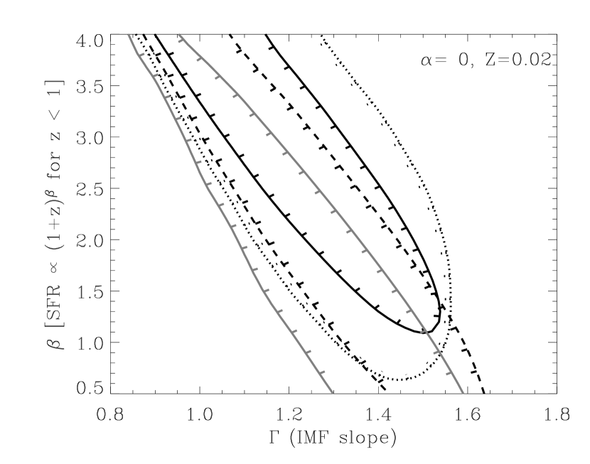
Figure 12: Confidence levels in $\beta$ versus $\Gamma$ for various dust approximations with the closed-box approximation. All the contours represent 95% 2-para. confidence limits. The dotted line represents the result from marginalizing over attenuation $A_{v}=0.2$–0.55 and $n=0.8$–1.2 (Sec. 3.4); the upper solid line from the fiducial $A_{v}=0.35$ and $n=1.0$ (effective average over many galaxies); the dashed line from fixed $A_{v}=0.75$ and $n=0.65$ (star-forming galaxies), and; the lower solid line from fixed $A_{v}=0.5$ with an MW extinction law (Pei, 1992).

4.3 Stellar mass, SFR and bolometric densities

We can calculate some derived physical properties of the Universe (at $z\approx 0.1$). The mass density in stars, $\Omega_{\rm stars}$, is in the range 1.1–2.0 $\times 10^{-3}$ $h^{-1}$, and; the SFR density, $\rho_{\rm SFR}$, is in the range 0.7–4.1 $\times 10^{-2}$ $h\,{\rm M}_{\odot}\,{\rm yr}^{-1}\,{\rm Mpc}^{-3}$. These ranges represent 95% confidence limits marginalized over IMF and cosmic SFH but restricted to near-solar metallicity models ($\bar{Z}$ or $Z=0.015$–0.025). However, the results depend strongly on the low-mass end of the stellar IMF which is not constrained by our analysis. As a test of the varying the low-mass end of the IMF, we also computed the ranges using the best-fitting IMFs and cosmic SFHs described in Table 2 (with $<95$% conf. of rejection). From these, $\Omega_{\rm stars}$ is in the range 0.8–2.5 $\times 10^{-3}$ $h^{-1}$, and; $\rho_{\rm SFR}$ is in the range 1.1–4.3 $\times 10^{-2}$ $h\,{\rm M}_{\odot}\,{\rm yr}^{-1}\,{\rm Mpc}^{-3}$. The lower stellar mass densities are derived from IMFs with $\Gamma_{m<1}\leq 0.5$ (Kennicutt, Salpeter mod. B, Scalo 1998) while the higher mass densities are derived from the Kroupa (2001) B IMF. The uncertainty in the current SFR density is not increased compared to the measurement based on the Equation 3 parameterization. The lowest SFR densities ($<0.01$) only occur in our models with $\Gamma\lesssim 1.1$ and none of the published IMFs in the table have $\Gamma_{m>1}<1.2$ which explains the lack of low SFR densities based on those IMFs.

These results are in good agreement with the results, based on the Kennicutt IMF, of Cole et al. and Baldry et al., and with the results, based on a modified Salpeter IMF, of Bell et al. (2003). They are generally not in agreement with results based on the Salpeter IMF extending down to 0.1 M_⊙ because such an IMF produces a high mass density from low mass stars that have minimal impact on the luminosity densities. This type of universal IMF is ruled out by stellar counts in the MW (e.g. Scalo, 1986, 1998) and by analysis of the dynamics of spiral galaxies (e.g. Bell & de Jong, 2001).

The total, bolometric, attenuated, stellar, luminosity density (0.09–5 $\mu$m) is determined from the models to be in the range 1.2–1.7 $\times 10^{35}$ $h\,{\rm W}\,{\rm Mpc}^{-3}$ (95% confidence). We can also estimate the total, bolometric, luminosity density ($\sim\,$5–1000 $\mu$m) due to dust absorbing and re-emitting stellar light. This depends critically on our dust model. From the best-fit models after marginalizing over dust-model parameters, the total is in the range 0.3–1.5 $\times 10^{35}$ $h\,{\rm W}\,{\rm Mpc}^{-3}$ which corresponds to 20–50% of the unattenuated stellar light being absorbed. If we restrict our dust model to ($A_{v}$,$n$) = (0.35,1.0), the ranges are 0.55–0.95 $\times 10^{35}$ $h\,{\rm W}\,{\rm Mpc}^{-3}$ and 30–40%.

From Saunders et al. (1990), the local, far-IR, 42–122 $\mu$m, luminosity density is in the range 0.17–0.26 $\times 10^{35}$ $h\,{\rm W}\,{\rm Mpc}^{-3}$ ($\pm 2\sigma$ range). This is significantly lower than the energy predicted by our dust model. However, a correction to total dust emission needs to be applied. Using the infrared energy dust models of Dale & Helou (2002), corrections from the 42–122 band emission to the total dust emission range from 1.9 to 2.6. If we assume this represents the systematic uncertainty in the luminosity density correction, then the total bolometric dust emission is in the range 0.3–0.7 $\times 10^{35}$ $h\,{\rm W}\,{\rm Mpc}^{-3}$ (scaling from the Saunders et al. result). Our fiducial dust model has a range in total bolometric emission that overlaps with this estimate.

This upper limit of 0.7 $\times 10^{35}$ $h\,{\rm W}\,{\rm Mpc}^{-3}$ for the dust emission favors models with lower attenuation and/or lower luminosity densities around 0.2 $\mu$m. From our fitting, after marginalizing over dust-model parameters, we obtain $A_{2000}\lesssim 1$. This is marginally inconsistent with the Sullivan et al. (2000) estimate of the effective attenuation, 1.3, which is why we have not used the estimated total dust emission to constrain our dust model. This discrepancy could be resolved if the UV luminosity density and/or attenuation were overestimated, and/or the total IR plus sub-mm flux was underestimated perhaps due to a population of galaxies with colder dust than those detected by 60 $\mu$m surveys. Note also that Buat & Burgarella (1998) found an average attenuation of 1.2 but this may not be inconsistent with our attenuation limit since it represents a limit on the luminosity-weighted average by flux. Future analyses could use IR and sub-mm luminosity density measurements to better constrain a dust model.

4.4 H$\alpha$ luminosity density

The H$\alpha$ nebular emission comes from reprocessed Lyman continuum photons. Therefore it provides a measure of the UV flux blueward of 0.1 $\mu$m. Here, we consider measurements of the attenuation-corrected H$\alpha$ luminosity density, relative to the ${}^{0.1}r$ band, in comparison with model predictions. This emission-line attenuation is significantly higher than for the stellar light at the same wavelength (Calzetti, Kinney, & Storchi-Bergmann, 1994) but it can be estimated using the Balmer decrement (H$\alpha$/H$\beta\approx 2.85$ for case B recombination, Hummer & Storey, 1987).

Table 3: Attenuation-corrected H$\alpha$ luminosity densities

reference	$\log(L_{H\alpha}\,/\,h{\rm\,W\,Mpc}^{-3})$	notes
Gallego et al. (1995)	32.39	$z\approx 0.03$, UCM objective-prism survey, luminosity function
Tresse & Maddox (1998)	32.74	$z\approx 0.20$, CFRS, luminosity function
Glazebrook et al. (2003)	32.77	$z\approx 0.03$, SDSS, cosmic spectrum

Three attenuation-corrected H$\alpha$ luminosity density measurements are summarized in Table 3. We do not quote error bars as the uncertainties are dominated by systematics. These include (i) subtraction of the stellar contamination which, in particular, affects the measurement of H$\beta$ and thus the estimate of the attenuation (Glazebrook et al. 2003 included this uncertainty which amounted to 0.1–0.15 in the $\log$ result), (ii) uncertainties in the attenuation curve (e.g. Caplan & Deharveng, 1986) which affect the conversion from a reddening measurement to absolute attenuation, and (iii) AGN contamination. Both the Gallego et al. (1995) and Tresse & Maddox (1998) results are based on obtaining the emission-line luminosity function from spectra. However, the selection criteria of the surveys are different, an emission-line objective-prism survey and $I$-band photometry, respectively. Glazebrook et al. (2003) took a different approach of summing SDSS spectra to form a cosmic optical spectrum before calculating the H$\alpha$ and H$\beta$ luminosity densities. We take the mean of these three results for our fitting:

$$\log(L_{H\alpha}\,/\,h{\rm\,W\,Mpc}^{-3})=32.63\pm 0.20\>.$$ (6)

This is appropriate since the Tresse & Maddox and Glazebrook et al. results may be too high due to AGN contamination which are enhanced by aperture affects. The spectra taken through a fiber are normalized to a broadband filter and since AGN are centrally concentrated, any emission line luminosity due to them will be over enhanced. However, Glazebrook et al. did measure the weak OI 6300 Å line, suggesting that the AGN contribution was only a few percent at most. The Gallego et al. result is probably too low because of the small survey (i.e. large scale structure) and/or because it only includes EW$>$10 Å (H$\alpha$, emission positive) galaxies.

To compare this average measurement with model predictions, we use the output from PEGASE for the H$\alpha$ flux without dust attenuation. As with the earlier fitting, the synthetic spectra are normalized to the ${}^{0.1}r$ band so we are really comparing the ratio of H$\alpha$ and ${}^{0.1}r$ band fluxes between the models and the data. A correction is made for the fact that the measured ${}^{0.1}r$ band flux includes dust attenuation because we are fitting to an attenuation-corrected H$\alpha$ measurement. We use the fiducial attenuation of $A_{v}=0.35$. In other words, unlike the earlier fitting we now normalize the synthetic spectra to an attenuation-corrected luminosity density in the ${}^{0.1}r$ band.

Figure 13 shows the results from fitting to the average attenuation-corrected H$\alpha$ luminosity density. The degeneracy in $\beta$ versus $\Gamma$ is similar to that for the broadband luminosity densities. In addition, the best-fit IMF slope, $\Gamma$ in the range 0.9–1.5 (68% conf. assuming $\alpha=0$ and averaging over the metallicity approximations), is in good agreement with the those results.

Figure 13: Confidence levels in $\beta$ versus $\Gamma$ from fitting solely to the H$\alpha$ luminosity density (Eqn. 6, relative to the ${}^{0.1}r$ band). The solid lines represent the contours for the closed-box approximation while the dotted lines represent the contours for the constant-metallicity approximation. The contours represent 68% 1-para. and 95% 2-para. confidence levels.

5 Conclusions

In this paper, we present the results of fitting spectral synthesis models with varying IMFs to local luminosity densities.

• A good fit is obtained to the measurements of Sullivan et al. (2000), Blanton et al. (2003b) and Cole et al. (2001) $K$-band (compilation SBC_K) with a best-fit metallicity of around solar. If we fit to the measurements of the first two papers and Huang et al. (2003) (compilation SBH), the best fit metallicity is greater than twice solar and the results are inconsistent with solar metallicity at the 99.7% confidence level.

• The data can be well fit by a universal IMF and, therefore, there is no need to invoke IMF variations. However, this provides only a weak constraint on the invariance of the IMF because of significant degeneracies associated with this type of modeling.

• The best-fit universal IMF slope marginalized over a significant range of cosmic SFH ($0.5\leq\beta\leq 4.0$, $-2\leq\alpha\leq 2$) is $\Gamma=1.15\pm 0.2$ based on an average between a closed-box approximation and a constant-metallicity approximation around solar (using compilation SBav). Our results are in good agreement with the Salpeter IMF slope.

• A strong upper limit of $\Gamma<1.7$ is obtained with 99.7% or 95% confidence depending on the metallicity approximation. This rules out the Scalo (1986) IMF for a universal IMF since the mass fraction of stars above 10 M_⊙ is similar to our parameterization with $\Gamma=1.8$ (Fig. 1, see also Table 2). A similar conclusion was reached by Madau et al. (1998) from fitting to luminosity densities over a range of redshifts and by Kennicutt et al. (1994) from fitting to H$\alpha$ EW-color relations for galaxies. Madau et al. found a Salpeter IMF or an IMF with $\Gamma=1.7$ provided adequate fits. Here, we find that the latter slope does not provide a good fit to luminosity densities. This is principally because we have used more accurate local luminosity density measurements. If we increase our $1\sigma$ uncertainties by 0.05 at all wavelengths then we obtain $\Gamma<1.7$ with 80% confidence.

• The stellar mass density of the universe is in the range 1.1–2.0 $\times 10^{-3}$ $h^{-1}$ based on marginalizing over cosmic SFH and our parameterization of the IMF. The current SFR density is in the range 0.7–4.1 $\times 10^{-2}$ $h\,{\rm M}_{\odot}\,{\rm yr}^{-1}\,{\rm Mpc}^{-3}$. The total bolometric stellar emission (0.09–5 $\mu$m) is known more accurately, naturally because we observe light and not mass, and is in the range 1.2–1.7 $\times 10^{35}$ $h\,{\rm W}\,{\rm Mpc}^{-3}$ derived from the fitted PEGASE model spectra (the mass-to-light ratio is $\sim 0.9$–1.4 M_⊙/L_⊙). We find that our dust model can reproduce the estimated total dust emission (0.3–0.7 $\times 10^{35}$ $h\,{\rm W}\,{\rm Mpc}^{-3}$, $\sim\,$5–1000 $\mu$m) scaled from the far-IR luminosity density (Saunders et al., 1990) if we have $A_{2000}\lesssim 1$ ($\lesssim\,$60%). Note that this represents a limit on the cosmic spectrum attenuation, i.e., a luminosity-weighted average by flux (not magnitudes).

• Fitting to the local H$\alpha$ luminosity density provides a similar result for the IMF slope ($\Gamma=1.2\pm 0.3$). This provides some evidence that our upper mass cutoff of 120 M_⊙ is a reasonable approximation because the sensitivity of the H$\alpha$ flux to massive stars is different to that of the mid-UV to optical fluxes. More accurate measurements could test this upper mass limit.

• The quantitative results on $\Gamma$ rely on the accuracy of the population synthesis model (PEGASE). An alternative, qualitative result would be that there is consistency between the theory of evolutionary population synthesis (evolutionary tracks and stellar spectra) and the measurements of luminosity densities, cosmic SFH and an average MW IMF derived from stellar counts (e.g. $\Gamma\approx 1.3$ from Kroupa, 2001).

Greater constraints can be placed on a universal IMF both by improved accuracy in local luminosity density measurements (in particular, $z=0.1$ to match the multi-wavelength SDSS MGS) and by improved accuracy of direct measures of cosmic SFH with redshift (in particular, $z=0$ to $z\sim 1$–2). For the direct tracing of cosmic SFH, it is important that the UV is measured at the same rest-frame wavelength in order to avoid IMF dependency. In other words, we need an IMF-independent cosmic SFH in order for the local luminosity densities to accurately constrain a universal IMF or the IMF-dependency should be quantified.

References

- Baldry et al. (2002) Baldry, I. K. et al. 2002, ApJ, 569, 582
- Barbaro & Poggianti (1997) Barbaro, G. & Poggianti, B. M. 1997, A&A, 324, 490
- Bell & de Jong (2001) Bell, E. F. & de Jong, R. S. 2001, ApJ, 550, 212
- Bell et al. (2003) Bell, E. F., McIntosh, D. H., Katz, N., & Weinberg, M. D. 2003, ApJ, submitted (astro-ph/0302543)
- Blanton et al. (2001) Blanton, M. R. et al. 2001, AJ, 121, 2358
- Blanton et al. (2003a) —. 2003a, ApJ, in press (astro-ph/0209479)
- Blanton et al. (2003b) —. 2003b, ApJ, in press (astro-ph/0210215)
- Bressan et al. (1993) Bressan, A., Fagotto, F., Bertelli, G., & Chiosi, C. 1993, A&AS, 100, 647
- Buat & Burgarella (1998) Buat, V. & Burgarella, D. 1998, A&A, 334, 772
- Calzetti (1997) Calzetti, D. 1997, in AIP Conf. Proc., Vol. 408, The Ultraviolet Universe at Low and High Redshift: Probing the Progress of Galaxy Evolution, ed. W. H. Waller (Woodbury: AIP), 403
- Calzetti (2001) —. 2001, PASP, 113, 1449
- Calzetti et al. (1994) Calzetti, D., Kinney, A. L., & Storchi-Bergmann, T. 1994, ApJ, 429, 582
- Caplan & Deharveng (1986) Caplan, J. & Deharveng, L. 1986, A&A, 155, 297
- Charlot & Fall (2000) Charlot, S. . & Fall, S. M. 2000, ApJ, 539, 718
- Charlot et al. (2002) Charlot, S., Kauffmann, G., Longhetti, M., Tresse, L., White, S. D. M., Maddox, S. J., & Fall, S. M. 2002, MNRAS, 330, 876
- Clegg & Middlemass (1987) Clegg, R. E. S. & Middlemass, D. 1987, MNRAS, 228, 759
- Cole et al. (2001) Cole, S. et al. 2001, MNRAS, 326, 255
- Colless et al. (2001) Colless, M. et al. 2001, MNRAS, 328, 1039
- Contini et al. (2002) Contini, T., Treyer, M. A., Sullivan, M., & Ellis, R. S. 2002, MNRAS, 330, 75
- Cowie et al. (1999) Cowie, L. L., Songaila, A., & Barger, A. J. 1999, AJ, 118, 603
- Cutri et al. (2001) Cutri, R. M. et al. 2001, Explanatory Supplement to the 2MASS Second Incremental Data Release (IPAC/Caltech)6662MASS explanatory supplement is available at http://www.ipac.caltech.edu/2mass/releases/second/doc/explsup.html
- Dale & Helou (2002) Dale, D. A. & Helou, G. 2002, ApJ, 576, 159
- Dey et al. (1998) Dey, A., Spinrad, H., Stern, D., Graham, J. R., & Chaffee, F. H. 1998, ApJ, 498, L93
- Elmegreen (1999) Elmegreen, B. G. 1999, ApJ, 515, 323
- Fioc & Rocca-Volmerange (1997) Fioc, M. & Rocca-Volmerange, B. 1997, A&A, 326, 950 (PEGASE)
- Fioc & Rocca-Volmerange (1999) —. 1999, PEGASE.2, astro-ph/9912179 (Institut d’Astrophysique de Paris)777Revised 2001 May. PEGASE.2 is available at http://www.iap.fr/users/fioc/PEGASE.html
- Gallego et al. (1995) Gallego, J., Zamorano, J., Aragon-Salamanca, A., & Rego, M. 1995, ApJ, 455, L1
- Gilmore & Howell (1998) Gilmore, G. & Howell, D., eds. 1998, ASP Conf. Ser., Vol. 142, The Stellar Initial Mass Function (San Francisco: Astron. Soc. Pacific)
- Glazebrook et al. (2003) Glazebrook, K. et al. 2003, ApJ, 587, 55
- Haarsma et al. (2000) Haarsma, D. B., Partridge, R. B., Windhorst, R. A., & Richards, E. A. 2000, ApJ, 544, 641
- Hammer et al. (1997) Hammer, F. et al. 1997, ApJ, 481, 49
- Haywood (2001) Haywood, M. 2001, MNRAS, 325, 1365
- Hogg (2002) Hogg, D. W. 2002, preprint (astro-ph/0105280v2)
- Huang et al. (1997) Huang, J.-S., Cowie, L. L., Gardner, J. P., Hu, E. M., Songaila, A., & Wainscoat, R. J. 1997, ApJ, 476, 12
- Huang et al. (2003) Huang, J.-S., Glazebrook, K., Cowie, L. L., & Tinney, C. 2003, ApJ, 584, 203
- Hummer & Storey (1987) Hummer, D. G. & Storey, P. J. 1987, MNRAS, 224, 801
- Kennicutt (1983) Kennicutt, R. C. 1983, ApJ, 272, 54
- Kennicutt (1998) —. 1998, in The Stellar Initial Mass Function, ed. G. Gilmore & D. Howell (San Francisco: ASP), 1
- Kennicutt et al. (1994) Kennicutt, R. C., Tamblyn, P., & Congdon, C. E. 1994, ApJ, 435, 22
- Kochanek et al. (2001) Kochanek, C. S. et al. 2001, ApJ, 560, 566
- Kogut et al. (2003) Kogut, A. et al. 2003, ApJ, submitted (astro-ph/0302213)
- Kroupa (2001) Kroupa, P. 2001, MNRAS, 322, 231
- Kroupa (2002) —. 2002, Science, 295, 82
- Kroupa et al. (1993) Kroupa, P., Tout, C. A., & Gilmore, G. 1993, MNRAS, 262, 545
- Kurucz (1992) Kurucz, R. L. 1992, in IAU Symp. 149, The Stellar Populations of Galaxies, ed. B. Barbuy & A. Renzini (Dordrecht: Kluwer), 225
- Lanzetta et al. (2002) Lanzetta, K. M., Yahata, N., Pascarelle, S., Chen, H., & Fernández-Soto, A. 2002, ApJ, 570, 492
- Lejeune et al. (1997) Lejeune, T., Cuisinier, F., & Buser, R. 1997, A&AS, 125, 229
- Lilly et al. (1996) Lilly, S. J., Le Fevre, O., Hammer, F., & Crampton, D. 1996, ApJ, 460, L1
- Madau et al. (1996) Madau, P., Ferguson, H. C., Dickinson, M. E., Giavalisco, M., Steidel, C. C., & Fruchter, A. 1996, MNRAS, 283, 1388
- Madau et al. (1998) Madau, P., Pozzetti, L., & Dickinson, M. 1998, ApJ, 498, 106
- Maddox et al. (1990) Maddox, S. J., Efstathiou, G., Sutherland, W. J., & Loveday, J. 1990, MNRAS, 243, 692
- Madgwick et al. (2002) Madgwick, D. S. et al. 2002, MNRAS, 333, 133
- Miller & Scalo (1979) Miller, G. E. & Scalo, J. M. 1979, ApJS, 41, 513
- Milliard et al. (1992) Milliard, B., Donas, J., Laget, M., Armand, C., & Vuillemin, A. 1992, A&A, 257, 24
- Norberg et al. (2002) Norberg, P. et al. 2002, MNRAS, 336, 907
- Oke & Gunn (1983) Oke, J. B. & Gunn, J. E. 1983, ApJ, 266, 713
- Pei (1992) Pei, Y. C. 1992, ApJ, 395, 130
- Rowan-Robinson et al. (1997) Rowan-Robinson, M. et al. 1997, MNRAS, 289, 490
- Salpeter (1955) Salpeter, E. E. 1955, ApJ, 121, 161
- Saunders et al. (1990) Saunders, W., Rowan-Robinson, M., Lawrence, A., Efstathiou, G., Kaiser, N., Ellis, R. S., & Frenk, C. S. 1990, MNRAS, 242, 318
- Scalo (1986) Scalo, J. M. 1986, Fundamentals of Cosmic Physics, 11, 1
- Scalo (1998) —. 1998, in The Stellar Initial Mass Function, ed. G. Gilmore & D. Howell (San Francisco: ASP), 201
- Schechter (1976) Schechter, P. 1976, ApJ, 203, 297
- Skrutskie et al. (1997) Skrutskie, M. F. et al. 1997, in The Impact of Large Scale Near-IR Sky Surveys (Dordrecht: Kluwer), 25
- Spergel et al. (2003) Spergel, D. N. et al. 2003, ApJ, submitted (astro-ph/0302209)
- Spitzer (1978) Spitzer, L. 1978, Physical processes in the interstellar medium (New York: Wiley-Interscience)
- Steidel et al. (1999) Steidel, C. C., Adelberger, K. L., Giavalisco, M., Dickinson, M., & Pettini, M. 1999, ApJ, 519, 1
- Stoughton et al. (2002) Stoughton, C. et al. 2002, AJ, 123, 485
- Strauss et al. (2002) Strauss, M. A. et al. 2002, AJ, 124, 1810
- Sullivan et al. (2000) Sullivan, M., Treyer, M. A., Ellis, R. S., Bridges, T. J., Milliard, B., & Donas, J. . 2000, MNRAS, 312, 442
- Tresse & Maddox (1998) Tresse, L. & Maddox, S. J. 1998, ApJ, 495, 691
- Treyer et al. (1998) Treyer, M. A., Ellis, R. S., Milliard, B., Donas, J., & Bridges, T. J. 1998, MNRAS, 300, 303
- Wolf et al. (2003) Wolf, C., Meisenheimer, K., Rix, H.-W., Borch, A., Dye, S., & Kleinheinrich, M. 2003, A&A, 401, 73
- Woosley & Weaver (1995) Woosley, S. E. & Weaver, T. A. 1995, ApJS, 101, 181
- Worthey (1994) Worthey, G. 1994, ApJS, 95, 107
- Wright (2001) Wright, E. L. 2001, ApJ, 556, L17
- Wyse (1997) Wyse, R. F. G. 1997, ApJ, 490, L69+
- York et al. (2000) York, D. G. et al. 2000, AJ, 120, 1579