THE KINEMATICS AND PHYSICAL CONDITIONS OF THE IONIZED GAS IN NGC 4593 FROM CHANDRA HIGH-ENERGY GRATING SPECTROSCOPY

Abstract

We observed the Seyfert 1 galaxy NGC 4593 with the Chandra high energy transmission gratings and present a detailed analysis of the soft X-ray spectrum. We measure strong absorption lines from He-like O, Ne, Mg, Si, H-like N, O, Ne, Mg, Si and highly ionized Fe xix-xxv. The weighted mean of the offset velocity of the strongest absorption profiles is $-140\pm 35$ km $\rm{s}^{-1}$. However the individual profiles are consistent with the systemic velocity of NGC 4593 and many profiles hint at the presence of either multiple kinematic components or blending. Only the N vii Ly$\alpha$ ($\lambda 24.781$) , O viii Ly$\alpha$ ($\lambda 18.969$) and Mg xii Ly$\alpha$ ($\lambda 8.421$) lines appear to be marginally resolved. We identify a spectral feature at $\sim 0.707$ keV with a neutral Fe L edge, which might suggest that there is dust along the line-of-sight to NGC 4593 although, this is not the only interpretation of this feature. A search for neutral O absorption which would reasonably be expected from dust absorption is complicated by contamination of the Chandra ACIS CCDs. Neutral Si absorption, which might also be expected from absorption due to dust is present (though not significantly) in the form of a weak neutral Si edge. The neutral Si column ($<4\times 10^{17}\ \rm{cm}^{-2}$) corresponding to the Si edge is consistent with the neutral Fe column ($\sim 1.5\times 10^{17}\ \rm{cm}^{-2}$) from the Fe L edge. We also detect, at marginal signficance, N vii Ly$\alpha$ ($\lambda 24.781$) and O vii (r) ${\it 1s^{2}-1s2p}$ ($\lambda 21.602$) absorption at $z\sim 0$, due to a hot medium in our Local Group. The soft X-ray spectrum of NGC 4593 is adequately described by a simple, single-zone photoionized absorber with an equivalent Hydrogen column density of $5.37^{+1.45}_{-0.79}\times 10^{21}\ \rm{cm}^{-2}$ and an ionization parameter of $\log\xi=2.52^{+0.06}_{-0.04}$ ergs cm $\rm{s}^{-1}$ although there remain some features which are not identified. Although the photoionized gas almost certainly is comprised of matter in more than one ionization state and may consist of several kinematic components, data with better signal-to-noise ratio and better spectral resolution are required to justify a more complex model. Finally, in emission we detect only weak forbidden lines of [Ne ix] and [O vii] .

1 Introduction

The launch of Chandra and XMM-Newton began a new era in the study of X-ray photoionized circumnuclear gas. High resolution X-ray spectroscopy with Chandra now allows the gas kinematics to be studied seriously for the first time, and the detection of individual absorption and emission lines can now place very strong constraints on the ionization structure of the warm, or partially ionized, X-ray absorbing gas in type 1 active galactic nuclei (AGNs)(e.g. Lee et al. (2001); Sako et al. 2001a ; Kaastra et al. (2002); Kaspi et al. (2002); Yaqoob et al. (2003)).

Here we present the results of a Chandra High-Energy Transmission Grating (or HETGS –Markert, et al. 1995) observation of NGC 4593 , which was simultaneous with an RXTE observation. NGC 4593 ($z=0.0083$, De Vaucouleurs et al. 1991) is a type I AGN that lies within a barred-spiral host galaxy. NGC 4593 is also relatively luminous ($L_{2-10\rm\ keV}$ typically $8.6\times 10^{42}\ \rm ergs\ s^{-1}$, converted from the luminosity given in Reynolds (1997) using $H_{0}=70\ \rm km\ s^{-1}\ Mpc^{-1}$ and $q_{0}=0$ which we use throughout this paper). In the present paper we focus on the soft X-ray spectroscopy results.

The paper is organized as follows. In §2 we present the data and describe the analysis techniques. In §3 we discuss gross features of the X-ray spectrum, including the intrinsic continuum form and interpret the data in the context of historical, lower spectral resolution CCD data. In §4 we qualitatively discuss the discrete X-ray spectral features before describing detailed spectral modeling. In §5 we describe in detail the modeling of the X-ray spectrum using the photoionization code, XSTAR. In §6 we compare our results with those from other X-ray observations of NGC 4593 . In §7 we discuss the possibility of a dusty warm absorber in NGC 4593 and we investigate the relativistically broadened disk-line scenario (Branduardi-Raymont et al. 2001; Sako et al. 2001b; Mason et al. 2002) as an alternative to the dusty warm absorber model. Finally, in §8 we summarize our results and in §9 briefly state our conclusions.

2 Observations and Data

We observed NGC 4593 with Chandra (simultaneously with RXTE ) on 2001 June 29 for a duration of $\sim 79$ ks, beginning at UT 00:54:49. The Chandra data were reprocessed using ciao 2.1.3 and CALDB version 2.7, according to recipes described in ciao 2.1.3 threads. The RXTE PCA data were reduced using methods described in Weaver, Krolik, & Pier (1998), except improved background subtraction was utilized (released 2002, February) and a later version of the spectral response matrix (v 8.0) was used. Only data from layer 1 and from PCUs 1, 2, 3 and 4 were used (PCU0 has had technical problems in the later part of the mission).

For Chandra the instrument used in the focal plane of the High Resolution Mirror Assembly was the HETGS . The HETGS consists of two grating assemblies, a High-Energy Grating (HEG) and a Medium-Energy Grating (MEG). Only the summed, negative and positive, first-order Chandra grating spectra were used in our analyis. For further discussion of the HETGS and our analysis procedure here, see Yaqoob et al. (2003). The mean Chandra total HEG and MEG count rates were $0.1965\pm 0.0017$ and $0.4743\pm 0.0021$ cts/s respectively. HEG, MEG and PCA spectra were extracted over the entire on-time for each instrument. This resulted in net exposure times of 78,889 s for HEG and MEG, and between $\sim 14$ ks and $\sim 70$ ks for each PCU. The background subtracted spectra from the different PCUs were co-added for analysis and the resulting mean count rate was 4.8 ct/s over the entire PCA band. The excess variances on the hardness ratios 1.0–2.5 keV/(0.6–1.0 keV) and 2.5–7.0 keV/(0.6–1.0 keV) for Chandra data binned at $0.16\AA$ were $0.0011\pm 0.0012$ and $0.0014\pm 0.0007$ respectively. Thus, the data are consistent with no spectral variability in soft X-rays during the observation, but there may be some small spectral variation in hard X-rays. The RXTE observation extended $\sim 20$ ks beyond the Chandra observation but the mean count rate in that portion of the observation was compatible with the mean of the strictly overlapping portion. Therefore, for the sake of improved statistics, the PCA spectrum included $\sim 10$ ks exposure beyond the Chandra data.

For Chandra HETGS we made effective area files (ARF, or ancillary response file), photon spectra and counts spectra following the method of Yaqoob et al. (2003). Since the MEG soft X-ray response is much better than the HEG (whose bandpass only extends down to $\sim 0.8$ keV) we will use the MEG as the primary instrument but refer to the HEG for confirmation of features in the overlapping bandpass and for constraining the continuum. The MEG spectral resolution corresponds to FWHM velocities of $\sim 280,560$, and 3,560 $\rm km\ s^{-1}$ at observed energies of 0.5, 1.0, and 6.4 keV respectively.

We did not subtract detector or X-ray background since it is such a small fraction of the observed counts ($<0.5\%$ for the MEG). We treated the statistical errors on both the photon and counts spectra with particular care since the lowest and highest energies of interest can be in the Poisson regime, with spectral bins often containing a few, or even zero counts. We assign statistical upper and lower errors of $1.0+\sqrt{(N+0.75)}$ and $N(1.0-[1.0-(1/9N)-(1/3\sqrt{(}N))]^{3})$ respectively (from Gehrels, 1986) on the number of photons, $N$, in a given spectral bin. Statistical errors were always computed on numbers of photons in final bins, according to the above prescription for plotting purposes. When fitting the Chandra data, we used the $C$–statistic (Cash, 1976) for finding the best-fitting model parameters, and quote 90$\%$ confidence, one-parameter statistical errors unless otherwise stated. The $C$–statistic minimization algorithm is inherently Poissonian and so makes no use of the errors on the counts in the spectral bins described above.

For the HEG data, the signal-to-noise ratio per $0.02\AA$ bin is $>1$ blueward of $\sim 15\AA$ and as high as $\sim 10$ in the $\sim 6-7\AA$ range. For the MEG data, in the $\sim 2-25\AA$ band which we examine here, the signal-to-noise ratio per $0.02\AA$ bin ranged from $\sim 1$ at $\sim 22.5\AA$ to a maximum of $\sim 14$ at $\sim 7\AA$. The systematic uncertainty in the energy scale is currently believed to be $0.0028\AA$ and $0.0055\AA$ for the HEG and MEG respectively. For the MEG, at 0.5 keV, 1 keV and 6.4 keV this corresponds to velocity offsets of $\sim 67$, 133, and 852 $\rm km\ s^{-1}$ respectively, and about half of these values for the HEG.

In addition, there has been a continuous degradation of the quantum efficiency of Chandra ACIS due to molecular contamination. The degradation includes an excess absorption due to neutral O . When fitting photoionization models to the data we will investigate the effect of this degradation on model parameters. There is no satisfactory correction available for the gratings but we will estimate worst case effects using a pure ACIS correction, since a grating in front of the CCDs will not make the CCD degradation worse. Indeed a grating may improve the situation by adding extra energy information. We will show in §5.3 that omitting the correction only affects the inferred intrinsic continuum and does not affect the important physical parameters of absorption models.

3 Overall Spectrum and Preliminary Spectral Fitting

We used XSPEC v11.2.0 for spectral fitting to the HEG and MEG spectra in the 0.8–5 keV and 0.5–5 keV bands respectively. These energy bands will be used in all the spectral fitting in the present paper, in which we concentrate on features in the soft X-ray spectrum (less than $\sim 2$ keV). The harder spectrum out to $\sim$ 15 keV, including the Fe-K emission line and Compton-reflection continuum (using simultaneous RXTE data in addition to the Chandra data) will be discussed elsewhere. However, we will utilize a portion of the RXTE PCA spectrum to constrain the continuum for fitting the soft X-ray Chandra data and use the $\chi^{2}$ statistic for minimization.

Since we convolve all models through the instrument response before comparing with the data, all our model line-widths are intrinsic values and do not need to be corrected for the instrument broadening. This contrasts with the analysis method in some of the literature on results from grating data in which models are fitted directly to the data and then corrected for instrument broadening (e.g. Kaspi et al. 2002). First, we show how the 0.5–5 keV MEG data compare to a simple model consisting only of a single power law and Galactic absorption. For the latter, we use a value of $1.97\times 10^{20}{\rm cm^{-2}}$ (Elvis et al. 1989) throughout this work. Later in this paper we show that the ACIS degradation discussed above does not effect our results. Therefore we do not let the Galactic column vary in spectral fitting since its systematic error is much less than the effects of ACIS degradation. Fig. 1 (a) shows the MEG photon spectrum of NGC 4593 binned at $0.32\AA$ (which is comparable with ASCA resolution) with the model overlaid. The power-law index was allowed to vary in this fit. Fig. 1 (b) shows the ratio of the data to this model. This simple power law is clearly a poor fit to the data, with considerable complexity apparent, both in the continuum, and in terms of discrete absorption features. Fig. 1 (b) clearly shows a soft X-ray excess, rising up from the hard power law (modified by Galactic absorption), below $\sim 0.7\ {\rm keV}$. We caution that there may still be broad residual uncertainties of $\sim 30\%$ or more in the calibration of the MEG effective area at the lowest energies . The instrumental effective area is very small at these energies, although residuals at $<0.6$ keV probably coincide with the complex instrumental O i edge which is spread over $\sim$ 10 eV around $\sim 0.53$ keV.

Observations of NGC 4593 in 1994 with ASCA , as summarized in Reynolds (1997) and George et al. (1998) also indicated a soft excess present below $\sim 0.7$ keV, relative to an extrapolation of the best-fitting hard X-ray power-law. A soft excess has also been observed by XMM-Newton and Chandra LETGS (Kaastra et al. 2001), as well as by BeppoSAX (Guainazzi et al. 1999). This would suggest that at least part of the soft excess we observed with Chandra HETGS is real. The low-energy degradation of the CCDs mentioned in §2 is in fact in the sense that any soft excess will actually be larger when the correction is taken into account.

The origin of the soft excess is unclear. It may be the tail end of some kind of soft thermal emission (or Comptonized soft thermal emission), possibly from an accretion disk (e.g. see Piro, Matt, & Ricci (1997), and references therein). Any relativistically-broadened O viii Ly$\alpha$ ($\lambda 18.969$) emission that is present could also contribute to the soft excess (e.g. Branduardi-Raymont et al. 2001; Turner et al. 2001). Since the soft excess appears only in the 0.5–1 keV band of our data, we do not have enough information to constrain its origin, and sophisticated modeling of it is not warranted. Therefore, in the remainder of this paper we model the 0.5–5 keV intrinsic continuum with a broken power law. When the data are modeled with this continuum, there is still considerable structure in the soft X-ray spectrum, characteristic of the presence of a photoionized, or ‘warm’ absorber.

Now, the warm absorber in NGC 4593 and other AGN when observed with CCDs (such as those on ASCA ) has often been modeled simply with absorption edges due to O vii and O viii since the lower CCD spectral resolution did not usually warrant more sophisticated models. In order to directly compare the new Chandra data with previous observations we modeled the MEG data for NGC 4593 with two absorption edges, Galactic absorption, and the intrinsic continuum described above. Here we used the RXTE PCA data to help constrain the continuum. First, we modeled the HEG, MEG, and PCA data simultaneously, the latter data only covering the 3–8 keV band in order to avoid the Compton-reflection continuum. We had to include an additional Gaussian model component (with center energy, width and intensity allowed to vary) to model the Fe-K line. Since we are not concerned with the Fe-K line in this paper we then take the hard power-law index ($\Gamma=1.794^{+0.013}_{-0.019}$) from this fit and use $\Gamma=1.794$ in all subsequent model-fitting in this paper. If we allow $\Gamma$ to vary in our best model (two absorption edges, a warm absorber and a broken power-law , see §8 below) fit to the Chandra MEG data binned at 0.16$\AA$, we find a best-fitting value of $\Gamma=1.803\pm 0.017$ which is consistent with the fixed value above, so fixing $\Gamma$ does not affect our results or conclusions. Since we will only be using Chandra data below 5 keV from this point on, we do not have to worry about the spectral fits becoming unstable due to too much interplay between the two parts of the broken power-law index and the Fe-K line model. This will be dealt with in future work.

In order to measure the absorption-edge parameters, we then modeled the 0.5–5 keV MEG data only, fixing the hard photon index at 1.794, and allowed the energies and optical depths (at threshold) of the two absorption edges to vary. The best-fitting model overlaid on the MEG photon spectrum is shown in Fig. 2 . Although a spectrum with bin size $0.04\AA$ was used for the spectral fitting, the plot shows the data binned at $0.32\AA$ since this is closer to the resolution of CCD data. The best-fitting parameters obtained from this model were $0.708\pm 0.003$ keV and $0.868^{+0.007}_{-0.010}$ keV for the edge threshold energies. For the the optical depths at threshold we obtained $\tau=0.18\pm 0.04$ and $0.14^{+0.03}_{-0.04}$ respectively. All quantities refer to the source rest frame. The best-fitting soft X-ray photon index was $2.26\pm 0.05$ and the break energy was $1.03^{+0.04}_{-0.03}$ keV.

The edge at 0.868 keV is in good agreement with the expected energy of the O viii edge at 0.871 keV. However, the edge at 0.708 keV is redshifted by $\sim 12,600$ km $\rm{s}^{-1}$ from the expected energy of the O vii edge (0.739 keV). Rather, this edge energy agrees extremely well with the expected energy of a neutral Fe L3-edge at 0.707 keV (as observed, for example, by Lee et al. (2001) in the warm absorber of MCG $-$6$-$30$-$15 ). Furthermore, adding a third edge to the continuum model, with a threshold energy fixed at that expected for O vii , does not improve the fit statistic significantly. The threshold optical depth of the O vii edge in this case is $<0.03$ at the one-parameter, $90\%$ confidence level. We note that since the spectrum is so complex around the regions of the O vii and O viii edges, optical depths derived from simple models should be interpreted with caution. We can compare the threshold optical depths with those measured from the 1994 January 4 ASCA observation of NGC 4593 (Reynolds 1997): $0.26\pm 0.04$ (ascribed to O vii ) and $0.09^{+0.04}_{-0.03}$ (O viii ). The Chandra and ASCA O viii edge depths are in marginal agreement but the O vii depths are completely incompatible. It seems that, due to the limited energy resolution of CCD data, the Fe-L3 edge was misidentified with an O vii edge, not only in NGC 4593 but possibly also for other AGN. The high resolution of Chandra HETGS indicates that this edge cannot be due to O vii , and previous ASCA data from AGN needs to be re-examined in this context. The optical depth that we measure for the Fe-L3 edge is in marginal agreement with that ascribed to the O vii edge by Reynolds (1997). The ASCA SIS (4-CCD mode) observation of NGC 4593 had an energy resolution (FWHM) of $\sim 140$ eV at $\sim 1.0$ keV at the time of the observation, and therefore could not distinguish between an O vii edge and a neutral Fe edge. However, an Fe-L edge for the feature at 0.7 keV is not the only interpretation (see §7). High resolution observations with Chandra are also hinting at X-ray absorption fine structure (XAF) around absorption edges (Lee et al. 2002). The apparent Fe-L edge in our data extends over $\sim 5$ eV, which is $\sim 3$ times the FWHM resolution of Chandra at this energy. The S/N of our data and the FWHM resolution of Chandra are not adequate to measure the XAF structure around the Fe-L edge, which in any case, will be complicated by O vii ${\it 1s^{2}-1snp}$ ($n>4$) absorption features.

4 Spectral Features and Kinematics

4.1 Absorption and Emission Lines

In order to best illustrate different characteristics of the spectrum we display the spectral data in several different ways. In Fig. 3 we show the MEG photon spectrum between 0.47–2.1 keV, as a function of observed energy. The data and the models in Fig. 3 are all absorbed by the Galactic column density. An important point to realize from Fig. 3 is that in some regions the spectrum is so complex that it is difficult to distinguish absorption from emission. For example, two emission features may be present between 1.0–1.5 keV according to the data/model ratio plot of Fig. 2 . However, from Fig. 3 it is clear that the peak flux of both features coincides with the inferred intrinsic continuum, implying that the apparent feature is simply due to the presence of broad absorption complexes on either side of it. In addition there is a sharp variation in the MEG effective area (at $\sim 0.85$ keV) and any uncertainties in the response could be manifested as an apparent spectral feature (see §5 for further discussion).

In Fig. 4 and Fig. 5 we show the MEG spectrum, this time as a function of wavelength in the source rest-frame, redward of $2\AA$. These spectra have bin sizes of $0.02\AA$, approximately the FWHM MEG spectral resolution ($0.023\AA$). In Fig. 4 we overlay the Lyman series (blue) for H-like N, O, Ne, Mg, Si, S, Ar and the corresponding He-like triplets (red) that lie in the 2-25$\AA$ range. In Fig. 5 we overlay the He-like resonance series lines (blue) to the $n=1$ level for the same elements. In addition, in Fig. 5 we indicate L-shell transitions of Fe xix (red) in the $2-25\AA$ range to illustrate just some of the blending of spectral features that can arise due to absorption by highly ionized Fe.

Referring to Figs. 3 to 5, we see that the strongest, clear discrete spectral features detected are absorption lines due to O viii Ly$\alpha$ ($\lambda 18.969$) , O viii Ly$\beta$ ($\lambda 16.006$) , Ne ix (r) ${\it 1s^{2}-1s2p}$ ($\lambda 13.447$), Ne ix (r) ${\it 1s^{2}-1s3p}$ ($\lambda 11.549$), Ne x Ly$\alpha$ ($\lambda 12.134$) , Mg xii Ly$\alpha$ ($\lambda 8.421$) , Si xiii (r) ${\it 1s^{2}-1s2p}$ ($\lambda 6.648$). Also included amongst the strongest discrete features are transitions (and blends of transitions) which we identify with highly ionized Fe, typically L-shell transitions in Fe xx –Fe xxv . Weaker absorption lines are also apparent from the spectra such as N vii Ly$\alpha$ ($\lambda 24.781$) , O vii (r) ${\it 1s^{2}-1s2p}$ ($\lambda 21.602$) and higher-order Lyman and (He-like) resonance absorption lines of O and Ne (there is evidence for transitions up to $n=4$ in each case; see Figs. 4 and 5). Some of these weaker features may be blended with Fe xxii - Fe xxiii transitions. Higher signal-to-noise X-ray spectroscopy (e.g. of NGC 3783, Kaspi et al. 2002) has shown that blending of absorption features considerably complicates the spectrum. In particular, transitions of Fe xxiii could be blended with the absorption troughs at $\sim 10.65$ and $11.0\AA$. Similarly, transitions of Fe xx and Fe xxii could be blended with troughs at $9.15\AA,12.8\AA$, and $11.75\AA$ respectively. We note that such a wide range of observed ionization states (from N vii to Fe xxv ) suggests that there is more than one ionization component of the warm absorber. We shall return to this point in the discussion of photoionization modeling in §5.

We also identify absorption features due to O vii (r) ${\it 1s^{2}-1s2p}$ ($\lambda 21.602$) and N vii Ly$\alpha$ ($\lambda 24.781$) in the observed frame, at $z=0$, indicating absorption along the line of sight due to a hot medium in our Galaxy or local group (see also Figs. 3, 4 & 5). The separations of the lines at $z=0$ and $z=0.0083$ is 2490 km $\rm{s}^{-1}$, which is easily resolved by Chandra . Strong local absorption by O vii (r) ${\it 1s^{2}-1s2p}$ ($\lambda 21.602$) and Ne ix (r) ${\it 1s^{2}-1s2p}$ ($\lambda 13.447$) and weaker local absorption by O viii Ly$\alpha$ ($\lambda 18.969$) and O vii (r) ${\it 1s^{2}-1s3p}$ ($\lambda 18.628$) has also been observed by Nicastro et al. (2002) in the direction of the blazar PKS 2155-304. Nicastro et al. (2002) suggest that the local absorption is produced in a low density intergalactic plasma, collapsing towards our Galaxy. It is likely that the $z=0$ absorption features O vii (r) ${\it 1s^{2}-1s2p}$ ($\lambda 21.602$) and N vii Ly$\alpha$ ($\lambda 24.781$) in NGC 4593 are due to the same gas. The strengths of the lines, although only marginally significant, are comparable with the EW$\sim 0.2-0.3$ eV detected by Nicastro et al. (2002).

Apart from Fe K$\alpha$ (which will be discussed elsewhere), we also identify weak [O vii] and [Ne ix] emission features. Table 1 shows that [O vii] and [Ne ix] are redshifted but the errors are consistent with systemic velocity. The corresponding intercombination and resonance lines of the O vii and Ne ix He-like triplets are not detected. The relative prominence of forbidden lines compared to the intercombination and resonance lines indicates an origin in a photoionized plasma (e.g. Porquet & Dubau 2000). Fig. 6 shows close-ups of the wavelength regions spanning the O vii and Ne ix He-like triplets (with the positions of the forbidden (f), intercombination (i) and resonance (r) lines marked in red). The ratio of the forbidden and intercombination line fluxes (R=f/i) constrains the electron density (e.g. see Porquet & Dubau 2000). An estimate of R from the flux at the i,f wavelengths in Fig. 6 yields R$<$3 for Ne ix and R$<$10 for O vii . These ratios imply $n_{e}<2\times 10^{12}\ {\rm cm^{-3}}$ and $n_{e}<8\times 10^{10}\ {\rm cm^{-3}}$ respectively, for a relative ionic abundance of the H-like and He-like ions of $\leq 10^{3}$ (see Fig.9 of Porquet & Dubau 2000). If blending is significant in either of these triplets, then the measured line intensities would be upper limits only, thereby yielding a potentially significant systematic error to our estimates of R and therefore $n_{e}$.

The presence of broad, bound-free absorption features and many narrow features which may be blended, makes it impossible to define an observed continuum for much of the spectrum, and therefore it is difficult to measure meaningful equivalent widths of even the strongest narrow absorption features. Rather than try to measure equivalent widths of all candidate features, and compare with model predictions, we will take the physically more direct approach of fitting photoionization models to the data (§5). First we give the measured energies and equivalent widths of the strongest absorption lines. The measurements were made using the broken power law plus two-edge model as the baseline spectral model (see §3) and Gaussians to model the absorption lines. The continuum and edge parameters were frozen at the best-fitting values given in §3, and the data were fitted over a few hundred eV centered on the feature of interest. Allowing the edge parameters to vary did not change our results. The fitted range of the data was extended down to 0.47 keV in order to measure the parameters of N vii Ly$\alpha$ ($\lambda 24.781$) . Initially the intrinsic width of each Gaussian was frozen at less than the instrumental resolution but then allowed to vary in order to investigate whether the lines were resolved. The results for the measured energies, apparent velocity shifts relative to systemic, equivalent widths, intrinsic widths and the improvement in the fit-statistic, of these strongest absorption features are given in Table 1. Note that the quoted equivalent widths are relative to the intrinsic continuum (corrected for Galactic absorption). Again, we caution that the measured equivalents widths are subject to uncertainties in the continuum, line-blending, and any complexity in the line profile. It is instructive to compare line strengths with a physical model, so also in Table 1 are the predicted equivalent widths from the best-fitting photoionization model discussed in §5.

4.2 Absorption-Line Velocity Profiles

Table 1 shows that most of the measured absorption lines are blueshifted, with Gaussian-fitted centroids ranging from near systemic velocity to $\sim-$310 km $\rm{s}^{-1}$. The exceptions are Ne ix (r) ${\it 1s^{2}-1s2p}$ ($\lambda 13.447$) and Fe xx ($\lambda 12.817$). The former is redshifted, but the measurement is consistent with systemic velocity and the latter is likely blended with nearby Fe xx transitions (see below). Some of the velocity profiles of the absorption features in Table 1 appear to be more complex than Gaussian, as can be seen from an inspection of the profiles in Fig. 7 and Fig. 8. These velocity profiles were obtained from combined HEG and MEG data except for those transitions at $>17\AA$, which were determined using MEG data only, since they are out of the HEG bandpass. The profiles are centered with zero at the systemic velocity of NGC 4593 , with positive and negative velocities corresponding to redshifts and blueshifts respectively. Superimposed on the data are velocity spectra from the best-fitting photoionization model which will be discussed in detail in §5.

Fig. 7  (a) shows the velocity profile centered on the O viii Ly$\alpha$ ($\lambda 18.969$) absorption transition in the NGC 4593 rest-frame. A broad absorption trough can be seen between $\sim-$600 km $\rm{s}^{-1}$ and systemic, centered around $\sim-$300 km $\rm{s}^{-1}$. Fig. 7  (b) is centered around the Ne x Ly$\alpha$ ($\lambda 12.134$) transition and also exhibits a broad absorption profile from $\sim-$300 km $\rm{s}^{-1}$ to $\sim$ +100 km $\rm{s}^{-1}$. Fig. 7  (c) shows the velocity profile for Mg xii Ly$\alpha$ ($\lambda 8.421$) , which exhibits a broad absorption profile from $\sim-$500 km $\rm{s}^{-1}$ to $\sim$ +300 km $\rm{s}^{-1}$. Fig. 7  (d) shows the velocity profile for Si xiv Ly$\alpha$ ($\lambda 6.182$) . The Si xiv Ly$\alpha$ ($\lambda 6.182$) profile appears to be broader than the others, with a flat base between $\pm$ 600 km ${\rm s^{-1}}$. There is also apparent emission at +900 km $\rm{s}^{-1}$ relative to systemic for Si xiv Ly$\alpha$ ($\lambda 6.182$) . This is problematic since Si xiv Ly$\alpha$ ($\lambda 6.182$) emission at +900 km $\rm{s}^{-1}$ would be difficult to reconcile with the small redshifts (consistent with systemic) of the [O vii] and [Ne ix] emission features. All four profiles in Fig. 7 have widths that agree with the formal upperlimits in Table 1 ($\sim$ few hundred to $\sim$ 1000 km ${\rm s^{-1}}$ FWHM for all profiles, except the more complex and broader Si xiv Ly$\alpha$ ($\lambda 6.182$) profile which is $\sim 2000$ km ${\rm s^{-1}}$ FWHM ). Formal results from Gaussian fits indicate that both O viii Ly$\alpha$ ($\lambda 18.969$) and Mg xii Ly$\alpha$ ($\lambda 8.421$) are marginally resolved (see Table 1).

Fig. 8 shows the velocity profiles of some of the strongest resonance absorption features and the profile of a transition in highly ionized Fe. Superimposed are velocity spectra from the best-fitting photoionization model (solid lines) and from the 99$\%$ upper limits on this model (dashed lines, superimposed in Fig. 8  (b,c) only) (see §5 for further details). Fig. 8  (a) is centered on the Fe xx ($\lambda 12.817$) transition. Absorption is strong and spans $\sim-$300 km $\rm{s}^{-1}$ to $\sim$ +500 km $\rm{s}^{-1}$. The profile appears deeper on the redward side of systemic. This may be due to a second absorber kinematic component, or due to blending with a one or more Fe L-shell transitions. Formally, from Gaussian fits, this Fe blend is marginally resolved (see Table 1). Fig. 8  (b) is centered on the Ne ix (r) ${\it 1s^{2}-1s2p}$ ($\lambda 13.447$) transition. The absorption trough spans $\sim-$100 km ${\rm s^{-1}}$ to $\sim$ +300 km ${\rm s^{-1}}$. Also noticeable in Fig. 8  (b) is the sharp absorption feature at $\sim$ +1500 km ${\rm s^{-1}}$. This probably corresponds to a blend of Fe xviii ($\lambda 13.503$) and Fe xix ($\lambda 13.504$) L-shell transitions, which are at $\sim$ +1300 km ${\rm s^{-1}}$ offset in velocity space from Ne ix (r) ${\it 1s^{2}-1s2p}$ ($\lambda 13.4473$). Fig. 8  (c) shows the absorption velocity profile of Mg xi (r) ${\it 1s^{2}-1s2p}$ ($\lambda 8.421$). The profile minimum lies around $\sim-$230 km ${\rm s^{-1}}$, and the profile which spans $\sim-$600 km ${\rm s^{-1}}$ to systemic velocity, appears slightly broader on the blueward side, suggesting an unresolved kinematic component or an unresolved blend with (most likely) Fe xx L-shell ($\lambda 9.166-9.167$) transitions. Finally, Fig. 8  (d) is centered on the Si xiii (r) ${\it 1s^{2}-1s2p}$ ($\lambda 6.648$) transition which spans $\sim-$300 km ${\rm s^{-1}}$ to systemic velocity.

Just as for the equivalent widths, one should not interpret apparent velocity shifts too literally because, in addition to uncertainty in the continuum, the velocity profiles are complex and in fact can be different for different ions. The complexity may either be intrinsic or due to contamination from other absorption and/or emission features. Emission filling in the red side of absorption features can lead to saturated features appearing non-saturated (Kaspi et al. 2002). If all the lines listed in Table 1 were in fact P Cygni, the estimated outflow velocities in Table 1 would gain a systematic error of about half of the listed outflow velocities. Intrinsic complexity could also be due, for example, to the presence of several kinematic components, making different contributions to the overall profile. However, the fact that most features are consistent with systemic (see Table 1) is significant and those features that deviate strongly from systemic are likely affected by spectral complexity.

5 Photoionization Modeling

We used the photoionization code XSTAR 2.1.h to generate several grids of models of emission and absorption from photoionized gas in order to directly compare with the data. We used the default solar abundances in XSTAR (e.g. see Table 2 in Yaqoob et al. 2003).

5.1 The Spectral Energy Distribution

First we constructed a spectral energy distribution (SED) for NGC 4593 , as follows. Average radio, infrared (IR), optical and ultraviolet (UV) fluxes were obtained from Ward et al. (1987) and NED. The X-ray region of the SED is constructed from the intrinsic continuum derived from our Chandra HETGS data (described below). Flux measurements obtained from historical data (Ward et al. 1987, NED) are not in general contemporaneous. Nevertheless, the NGC 4593 SED appears to exhibit a peak in the IR-UV spectral region. Due to the large spectral variability however, the flux levels in this spectral region can span up to an order of magnitude at a given frequency. We attempted to crudely account for variability in this region of the NGC 4593 SED by generating two different SEDs. For the first SED (SEDa), we chose the highest envelope of the measurements in the IR-UV region from Ward et al. (1987). SEDa exhibits a prominent IR-UV bump as is evident in Fig. 9 (SEDa is the solid line). We then simply connected the optical/UV endpoint of the IR-UV bump at $\sim 10^{15}$ Hz to the X-ray portion of the SED with a straight line in log-log space. The second SED (SEDb) was generated simply by connecting the highest energy IR data point at $\sim 10^{13.9}$ Hz from Ward et al. (1987) to the X-ray portion of the SED, such that SEDb does not have a prominent bump in the IR-UV region. SEDb is represented in Fig. 9 by filled circles connected by a dashed curve. By constructing these two SEDs, we could investigate the effect of reasonable uncertainties in the IR-UV region on the X-ray photoionization models. Also shown for comparison in Fig. 9 is the lower envelope of the measurements in the IR-UV region from Ward et al. (1987) (dash-dot line).

To derive the X-ray portion of the SED, we fitted the data with a broken power law continuum and three absorption edges (as discussed in §3 above). The 0.5 keV intrinsic model flux was then simply joined onto the last UV (SEDa) and IR (SEDb) points of the lower-energy part of the SED by a straight line in log-log space. The hard X-ray power law was extended out to 500 keV. Note that we did not include any correction for the ACIS low energy CCD degradation as there is no satisfactory correction for grating data. Grids of photoionization models (see §5.2 below) were then generated using this SED. Also shown in Fig. 9 is the ‘mean AGN’ SED derived by Matthews & Ferland (1987) normalized to the ionizing luminosity of the NGC 4593 SEDa.

5.2 Model Grids

The photoionization model grids used here are two-dimensional, corresponding to a range in values of total Hydrogen column density, $N_{\rm H}$, and the ionization parameter, $\xi=L_{\rm ion}/(n_{e}R^{2})$. Here $L_{\rm ion}$ is the ionizing luminosity in the range 1 to 1000 Rydbergs, $n_{e}$ is the electron density and $R$ is the distance of the illuminated gas from the ionizing source. The grids were computed for equi-spaced intervals in the logarithms of $N_{\rm H}$ and $\xi$, in the ranges $10^{20-22}\ {\rm cm^{-2}}$ and $10^{1.5-4.0}$ erg cm ${\rm s^{-1}}$ respectively. From SEDa, we deduce that $L_{\rm ion}\sim 7\times 10^{44}$ ergs $\rm{s}^{-1}$ and therefore the lowest values of $n_{e},\log\xi$ in the grid yield $R\sim 150$ pc and the highest values of $n_{e},\log\xi$ in the grid yield $R\sim 7$ light-hours. This range in $R$ in the grid spans the expected location of the warm absorber. We computed grids with $n_{e}$ in the range $10^{2-11}\ {\rm cm^{-3}}$. For XSTAR models of the absorber, we confirmed that results from fitting the photoionization models to the X-ray data were indistinguishable for densities in the range $n_{e}=10^{2}\ {\rm cm^{-3}}$ to $10^{11}\ {\rm cm^{-3}}$. Hereafter we will use $n_{e}=10^{8}\ {\rm cm^{-3}}$ unless otherwise stated. Different density models will be important when we come to model the emission lines.

All models assumed a velocity turbulence ($b$-value) of $1$ $\rm km\ s^{-1}$, and since XSTAR broadens lines by the greater of the turbulent velocity and the thermal velocity, it is the latter which is relevant for these models. As the turbulent velocity increases, the equivalent width of an absorption line increases for a given column density of an ion. Therefore, to calculate model equivalent widths correctly one must know what the velocity width is (note that the $b$-value could represent all sources of line-broadening). We cannot simply extend the XSTAR model grids into another dimension (velocity width), and deduce a $b$-value directly from model-fitting, because we are limited by the finite internal energy resolution of XSTAR. The widths of the energy bins of the XSTAR model grids are in the range $\sim$ 200–600 km ${\rm s^{-1}}$. Our choice of velocity width ($b$-value corresponding to the thermal width) ensures that the energy resolution of XSTAR is the limiting factor and not the $b$-value itself. We will then need to take a rather more complicated approach to model-fitting (described in §5.3 below) and deduce a b-value appropriate for the data.

5.3 Model-Fitting

We proceeded to fit the MEG and HEG spectra simultaneously (binned at $0.04\AA$, which is approximately the upper limit on the FWHM of most of the strong absorption features in Table 1) , with all corresponding model parameters for the two instruments tied together, except for the relative normalizations. The intrinsic continuum was a broken power law (the hard photon index again fixed at 1.794) modified by absorption from photoionized gas (derived from SEDa, which has a prominent bump in the IR-UV region, see §5.1) and the Galaxy, as well as an absorption edge due to neutral Fe in the rest-frame of NGC 4593 . Excluding overall normalizations, there were a total of seven parameters, namely the column density of the warm absorber, $N_{H}$, the ionization parameter, $\xi$ and the redshift $z$ of the warm absorber, the energy E and maximum optical depth $\tau$ of the neutral Fe absorption edge, the intrinsic soft photon index, $\Gamma_{2}$ and the break energy of the broken power-law continuum, $E_{\rm B}$.

Our model-fitting strategy is more complicated than simply comparing the XSTAR model spectra with the data since the XSTAR spectra assume a certain line width ($b$-value), which itself is limited by the finite internal energy resolution of XSTAR. We chose $b=1\ \rm km\ s^{-1}$ in order that the energy resolution of XSTAR is the limiting factor. The result is that the equivalent widths of lines in the XSTAR spectra need to be calculated more rigorously using a line width ($b$-value) appropriate for the data. On the other hand, the ionic columns in the XSTAR models are robust from this point-of-view and do not depend on the velocity width. Therefore, after finding the best-fitting ionization parameter and warm-aborber column density from a global fit using the model described above, in § 5.5 we will deduce a $b$-value from a curve-of-growth analysis, using ionic column densities from the best-fitting global model. We will then construct detailed model profiles for each of the detected absorption lines.

The best-fitting parameters derived from the XSTAR global model fits were $N_{H}=5.37^{+1.45}_{-0.79}\times 10^{21}\ {\rm cm^{-2}}$ and $\log{\xi}=2.52^{+0.06}_{-0.04}$ ergs cm ${\rm s^{-1}}$. The broken power-law model corresponding to this best fit had a break energy of $E_{\rm B}=1.07^{+0.08}_{-0.07}\ {\rm keV}$ and a soft power-law photon index of $\Gamma_{1}=2.27^{+0.08}_{-0.07}$, values which are consistent with the SED that was used as input to the models. The absorption edge had an energy of $E=0.708\pm 0.002$ and a optical depth of $\tau=0.19\pm 0.04$. The photoionized absorber was offset by $-$140 $\pm$ 35 km $\rm{s}^{-1}$ from the systemic velocity of NGC 4593 , the weighted mean of the values for velocity offsets of absorption features in Table 1, excluding the Fe xx ($\lambda 12.817$) transition, which is skewed, likely due to blending. We found that a photoionization model based on SEDb (the SED without a prominent bump in Fig. 9 ) yielded best-fit parameters within the $90\%$ errors given above ($\Delta C\sim 4$ for no additional parameters). Only a small difference in results between SEDa and SEDb should be expected since the relevant ionizing continuum is mainly in the X-ray band. Since there are no significant differences between the photoionization model fits corresponding to each SED, hereafter all photoionization model fits shall refer to SEDa (which has a prominent bump in the optical/UV frequency range). Table 2 shows the ionic column densities predicted by our best-fitting model for a range of ions.

Fig. 10 shows the best-fitting model folded through the MEG response and overlaid onto the MEG counts spectrum. The lower panel of Fig. 10 shows the ratio of the data to the best-fitting model. Fig. 11 shows the actual best-fitting XSTAR model before folding through the instrument response. Fig. 12 shows the 68$\%$, 90$\%$, and 99$\%$ joint confidence contours of $\log{\xi}$ versus $N_{H}$. Overall, the fit is good and it is already apparent that the best-fitting parameters which describe the overall spectrum also give good fits to the most prominent absorption lines and edges. This can also be seen in Fig. 3 which shows the best-fitting model overlaid on the photon spectrum, and in Fig. 7 and Fig. 8 which show close-ups of the data and model (in velocity space), centered on particular atomic transitions. In Fig. 3 , some absorption features are discrepant with the model predictions, most notably Si xiii (r) ${\it 1s^{2}-1s2p}$ ($\lambda 6.648$). The data and model disagree here for two reasons; firstly, because the $b$-value used by XSTAR is not appropriate for the individual absorption features, as discussed above. Secondly, the data in Fig. 3 are binned at $0.08\AA$ which has combined the two minima in Fig. 7  (d) at $\sim-200$ km $\rm{s}^{-1}$ (which we identify with Si xiii (r) ${\it 1s^{2}-1s2p}$ ($\lambda 6.648$) and $\sim-1000$ km $\rm{s}^{-1}$ (unidentified) into a single deep feature.

The wavelength accuracy of the XSTAR atomic database is 5 m$\AA$, which corresponds to a velocity offset of 120 km $\rm{s}^{-1}$ at 1 keV. This offset is marginally less than the offset due to uncertainty in the MEG energy scale (5.5m$\AA$). We mentioned in §3 that the 2.0–2.5 keV region in the Chandra spectra suffers from systematics as large as $\sim 20\%$ in the effective area due to limitations in the calibration of the X-ray telescope absorption edges in that region . We therefore omitted the 2.0–2.5 keV regions of the Chandra spectra during the spectral fitting so that the fits would not be unduly biased. These and other instrumental features can be seen in the upper panel of Fig. 10 . All the MEG data in the 0.5–5 keV band are shown here, although the 2.0–2.5 keV region was omitted during spectral fitting. Other regions which have sharp changes in the effective area also show notable mismatches between data and model, but these are not as bad as in the 2.0–2.5 keV region.

The ACIS CCDs have been undergoing a continuous low-energy QE degradation, probably due to absorption by a cumulative build-up of contaminants. Unfortunately, at the time of writing, there is no correction available for grating data. There is however, a model of the contamination pertinent for pure ACIS data (without the gratings). We can use this model as a ‘worst case’ to estimate the effects on our photoionization modeling and conclusions. Thus, we repeated the spectral fitting described above with the addition of the ACIS QE degradation model in XSPEC v11.2 (acisabs), using the defaults for absorption by the contaminants C, H, O, and N in the ratio 10:20:2:1 by number of atoms. Remarkably, we found that the best-fitting $N_{H}$, $\log{\xi}$ and their associated statistical errors, were essentially indistinguishable from those obtained without the contamination model. What changed was the soft photon index, which increased to $3.04^{+0.04}_{-0.05}$. Even the break energy remained essentially the same. Thus, our photoionization modeling is driven by the discrete, narrow absorption features in NGC 4593 and is therefore robust to broadband calibration uncertainties. To determine why the degradation model did not change $N_{H}$ or $\xi$, we simulated data consisting of an absorbed power–law continuum with and without degradation respectively. We then fitted the data with and without the acisabs model. We found that when the simulated spectrum with no degradation was fitted with acisabs, $N_{H}$ did not increase, but the continuum steepened. This is because the degradation yields deep absorption edges which are not in the simulated data. We conclude that the real data have much less degradation than is assumed by the acisabs degradation model.

5.4 Curve-of-Growth Analysis

In order to determine the correct velocity width ($b$-value) of absorption lines for our models, we calculated curves-of-growth for different values of $b$ (see Fig. 13 ). The theoretical curves-of-growth in Fig. 13 indicate that the measured equivalent widths of $\sim 10^{-2.8}\lambda$ are most consistent with $b\sim 100-200$ km $\rm{s}^{-1}$. We also plotted the measured equivalent widths from Table 1 (converted to Angstroms) as a function of ionic column density (from the best-fitting XSTAR model described above) and overlaid these on the curves-of-growth (Fig. 13 ). For solar abundances, most of the measurements are consistent with $b\sim 200$ $\rm km\ s^{-1}$ within errors. Note that the predicted equivalent widths for $b=200$ $\rm km\ s^{-1}$ are shown in Table 1 so that they can be compared directly with the observed equivalent widths.

All of the plotted features in Fig. 13 are consistent with the curves of growth except for O vii (r) ${\it 1s^{2}-1s2p}$ ($\lambda 21.602$). The disagreement with the curves of growth may be indicating a second component for the warm absorber with lower ionization parameter. However, all of the other strong absorption features on Fig. 13 seem to be consistent with the curves of growth. One explanation for the discrepancy might be an absorber component consisting of highly ionized dust. From §3 we have seen that the data are consistent with an overabundance of neutral Fe, likely bound up in dust along the line-of-sight. The dust that lies closest to the AGN may well be highly ionized, contributing to a larger O vii column than expected from a simple single zone photoionization model. Certainly this could also explain several highly ionized Fe features in Fig. 3 that are not well fit by our best-fitting model in §5.3. Highly ionized dust can survive in warm, photoionized gas (see Reynolds et al. (1997) for further dicussion) although it seems probable in such scenarios that the warm material originates in the dusty cold material, which could be derived from a molecular torus.

5.5 Detailed Comparison of Data and Photoionization Model

In this section we compare in detail the best-fitting XSTAR photoionized absorber model and the data (refer to Fig. 3 for the spectrum, and to Fig. 7 and Fig. 8 for some velocity spectra). Note that although the best-fitting model was derived using spectra binned at $0.04\AA$, we can compare the model and data at higher spectral resolution, depending on the signal-to-noise of the feature in question. The strongest absorption-line features in the Chandra data are listed in Table 1. Fig. 3 shows that the best-fitting XSTAR model described above ($N_{H}=5.37\times 10^{21}\ \rm cm^{-2}$, $\log{\xi}=2.52$ ergs cm $\rm{s}^{-1}$ ) appears to underpredict the strength of several absorption lines. However, as outlined in §5.3, the equivalent widths of lines in the XSTAR spectra do not correspond to a ($b$-value) appropriate for the data. For example, Si xiii (r) ${\it 1s^{2}-1s2p}$ ($\lambda 6.648$) in Fig. 3 shows a large discrepancy between the model and the data, but Table 1 does not. A proper comparison between data and model for the stronger lines is described below.

The model velocity profiles in Fig. 7 (for four of the strongest absorption lines: O viii Ly$\alpha$ ($\lambda 18.969$) , Ne x Ly$\alpha$ ($\lambda 12.134$) , Mg xii Ly$\alpha$ ($\lambda 8.421$) & Si xiv Ly$\alpha$ ($\lambda 6.182$) were calculated using the appropriate $b$-value for the data (200 km $\rm{s}^{-1}$) and show reasonable agreement between data and model. In this case the model curves were calculated using the broken power-law and two-edge continuum described in §3, a Gaussian for the absorption line, with $\sigma=b/\sqrt{2}=141.4$ $\rm km\ s^{-1}$, and the predicted model equivalent width from Table 1. Fig. 8 , which shows the velocity profiles of some of the strongest resonance absorption features and the profile of a transition in highly ionized Fe, illustrates that the best-fitting XSTAR model under-predicts some features. However the lower limits on the best-fitting column density and ionization parameter at 99$\%$ confidence, yield ionic columns that give velocity profiles that are more consistent with the data for Ne ix (r) ${\it 1s^{2}-1s2p}$ ($\lambda 13.447$) and Mg xi (r) ${\it 1s^{2}-1s2p}$ ($\lambda 8.421$) (dashed lines in Fig. 8 ), without significant disimprovement of the profiles in Fig. 7 . Thus, in spite of the likely wide range of ionization states in the warm absorbing gas, a single-component photoionization model can give surprisingly good fits to the principal absorption lines.

There are many more discrete absorption features apparent in the spectra but with lower signal-to-noise. Although these individual weak features cannot be studied in detail we can at least check whether the best-fitting XSTAR model does not conflict with the data. We found that, as far as narrow absorption lines are concerned, most absorption lines predicted by the model were consistent with the data. In particular, we found that the model agrees well with the data for the low-order Lyman and He-like resonance transitions of Ne and O, although there may be blending associated with higher order transitions such as Ne ix ${\it 1s^{2}-1s4p}$ ($\lambda 11.000$). Conversely, the data show possible strong absorption features which are not predicted by the model. These features are mainly in the $\sim 1.1-1.5$ keV range (e.g. see Fig. 3  (d)). Some of the strongest features may correspond to blends of L-shell transitions in very highly ionized Fe (Fe xx -Fe xxv ). The atomic database used by XSTAR 2.1.h does not yet include all transitions in highly ionized Fe and this would certainly explain these discrepancies between data and model.

The Fe ionic columns predicted by the best-fitting XSTAR model are largest for ionization states Fe xix to Fe xxiv . According to Behar, Sako, & Khan (2001), an Fe M-shell unresolved transition array (UTA) due to Fe i-Fe xv lies between 17.5$\AA$ and 15$\AA$. According to Gu et al. (2001), there is a strong L-shell signature due to Fe xx - Fe xxiv between 10.5$\AA$ and 12.5$\AA$. Thus, some of the strong absorption features between 0.85-1.0 keV in Fig. 3 may be part of, or blended with, an Fe UTA due to highly ionized Fe (our Fe ionic columns are largest for Fe xix - Fe xxv ). UTAs due to less highly ionized Fe (in the $\sim$ 15-17$\AA$ range) have been detected in some other Seyfert 1 galaxies (IRAS 13349$+$2438, Sako et al. 2001a; MCG $-$6$-$30$-$15, Lee et al. 2001; NGC 3783, Kaspi et al. 2002; NGC 5548, Kaastra et al. 2002; Mkn 509, Yaqoob et al. 2003).

In §3 we mentioned how spectral fits using simple absorption-edge models (representing O vii and O viii) could be misleading. We see that more sophisticated modeling with better data also gives a weak O vii edge, as obtained from edge-fitting, but also a much weaker O viii edge since the data above the O viii edge are affected by other absorption features (Fe UTAs and Ne ix (r) ($\lambda 13.447$) in particular) which can be accounted for by the photoionization models. This has also been pointed out by Lee et al. (2001). The complex of O vii $1s^{2}-1snp$ resonance transitions with $n>5$ may also complicate the region just above the O vii edge (see also Lee et al. 2001). From the XSTAR models we can extract the O vii and O viii ionic column densities at the extremes of the $90\%$ confidence intervals for $N_{H}$ versus $\xi$. We find that the O vii column is $4.0^{+2.6}_{-1.8}\times 10^{15}\ {\rm cm^{-2}}$ and the O viii column is $2.7^{+1.2}_{-0.8}\times 10^{17}\ {\rm cm^{-2}}$. Given an absorption cross-section at threshold of $2.4\times 10^{-19}\ \rm{cm^{-2}}$ for O vii and $9.9\times 10^{-20}\ \rm{cm^{-2}}$ for O viii (Verner et al. , 1996), we find that the model optical depths (at threshold) of the O edges are $\tau_{{\rm O~{}{\sc vii}}}=0.001^{+0.0006}_{-0.0005}$ and $\tau_{{\rm O~{}{\sc viii}}}=0.026^{+0.013}_{-0.007}$ respectively. These values can be compared with those obtained from an ASCA observation of NGC 4593 in 1994, in which simple ‘edge-models’ yielded $\tau_{{\rm O~{}{\sc vii}}}=0.26\pm 0.04$ and $\tau_{{\rm O~{}{\sc viii}}}=0.09^{+0.04}_{-0.03}$ (Reynolds (1997); see also George et al. 1998). Whilst the ASCA result is inconsistent with our inferred O vii optical depth, it is consistent with the optical depth of our best fit neutral Fe L edge ($\tau=0.19\pm 0.04$). Note that ASCA resolution at energies around 0.7 keV is too coarse to resolve the two edges separately (see discussion in §3). From an Fe L3 edge depth of $0.19\pm 0.04$, and given an Fe 2p absorption cross-section of $1.25\times 10^{-18}\rm{cm}^{-2}$ (Verner et al. 1996), we infer a neutral Fe column of $1.5\pm 0.3\times 10^{17}\ \rm{cm}^{-2}$. An Fe L1 (2s) edge (rest energy of 0.845 keV) optical depth of $\tau<0.05$ is allowed by the data, implying a neutral Fe column of $<3.6\times 10^{17}\rm{cm}^{-2}$ which is consistent with the estimate from the Fe L3 edge, although we caution that the spectrum at both the Fe L1 and the Fe L2 (rest energy of 0.720 keV) edge energies is complex. Indeed, we cannot derive a reasonable constraint on the Fe L2 edge optical depth because of apparent emission blueward of this edge (see Fig. 3 ). The implied neutral column density for cosmic abundances is then $N_{H}\sim 3.8\times 10^{21}\ {\rm cm}^{-2}$, which would act to extinguish the soft X-ray spectrum. Therefore the neutral Fe could take the form of neutral dust, as argued by Lee et al. (2001). Our estimate of the O viii optical depth from the photoionization modelling is inconsistent with both the ASCA result and our direct fit of the O viii edge ($\tau=0.14^{+0.04}_{-0.03}$). However, the XSTAR model fits the data well, so simple edge models may give the wrong optical depth. Nevertheless, we find that the measured equivalent widths of the O vii (r) ${\it 1s^{2}-1s2p}$ ($\lambda 21.602$) and O viii Ly$\alpha$ ($\lambda 18.969$) absorption lines in Table 1 yield ionic column densities that are consistent with the edge optical depths measured in §3.

We investigated the robustness of the XSTAR model fits to the absorption features by examining the data versus model at the extremes of the $N_{H}$ versus $\xi$ confidence intervals (see Fig. 12 ). By picking pairs of values of $N_{H}$ and $\xi$ in the plane of the contours, we can freeze the column density and ionization parameter at the chosen values and find the new best-fit for each pair of values (this is in fact how such contours are constructed). Then we can examine the data and model spectra in detail for each of these new fits to see where the model and data deviate significantly from each other. We found that the models were still able to account for the strengths of all of the strong absorption-line features (listed in Table 1) for pairs of $N_{H}$ and $\xi$ lying inside the 99$\%$ confidence contour. On the other hand, for pairs of $N_{H}$ and $\xi$ lying outside the 99$\%$ contour we found that absorption lines in the 12-15$\AA$ range were particularly sensitive and the equivalent width would be over-predicted or under-predicted by as much as a factor of two. Therefore, we conclude that the 99$\%$ confidence contours in Fig. 12 are a good guide to the allowed range of $N_{H}$ and $\xi$.

As well as absorption, the XSTAR code also calculates emission spectra. However, the very weak [Ne ix] and [O vii] forbidden lines that we observe (see Fig. 6 ) cannot constrain the XSTAR emission spectra. Therefore our best-fit photoionization model of the warm absorbing gas (Fig. 11 ) does not warrant inclusion of the corresponding (weak) emission spectrum. Stronger emission features have been detected in other observations of NGC 4593 and we shall discuss potential constraints on the emission region from previous observations in §6 below. The possibility of very broad relativistic emission lines in our soft X-ray data shall also be discussed in detail in §7.

6 Comparison with previous observations

Over the past decade NGC 4593 has been observed in X-rays, by ASCA on 1994 January 9, BeppoSAX from 1997 December 31 to 1998 January 2 and most recently, by XMM-Newton and Chandra LETGS (non-simultaneously on 2000 July 2 and 2001 February 16 respectively). We measured a 2–10 keV flux of $4.0\times 10^{-11}$ ergs $\rm{cm}^{-2}$ $\rm{s}^{-1}$ from NGC 4593 with Chandra HETGS . This is comparable with the flux detected by BeppoSAX (Guainazzi et al. 1999) and ASCA (Reynolds 1997). Using Fig.1 of Kaastra & Steenbrugge (2001), we find compared to the Chandra LETGS and XMM-Newton observations, our MEG flux at $20\AA$ is a factor $\sim 1.6$ and $\sim 1.9$ higher respectively. We compared our soft X-ray measurements with those from the ASCA observation in §3 and shall not discuss the ASCA results further. BeppoSAX observed a similar underlying continuum to that observed by us with Chandra HETGS . When the BeppoSAX continuum is fit with a simple powerlaw model ($\Gamma=1.70\pm 0.04$), the main deviations include an absorption feature at $\sim$ 0.7 keV and an apparent soft excess between $\sim$ 0.3–0.7 keV. Guainazzi et al. (1999) measured two edges whose threshold energies and optical depths are consistent with the Chandra Fe L and O vii measurements.

A strong soft excess was also observed by Chandra LETGS at energies less than $\sim 0.65$ keV, when the power law describing the LETGS data at $1-10\AA$ is extrapolated to lower energies. The Chandra LETGS data also exhibit a flux deficit between $\sim 0.65-1.2$ keV relative to the extrapolated powerlaw. Kaastra & Steenbrugge (2001) claim that the Chandra LETGS spectrum exhibits few strong discrete emission or absorption features, unlike our data. We note from Fig. 1 in Kaastra & Steenbrugge (2001) (which shows counts spectra versus observed wavelength between 18-23$\AA$), that the Chandra LETGS spectrum does exhibit some absorption features. There is weak absorption due to O vii (r) ${\it 1s^{2}-1s2p}$ ($\lambda 21.602$), a weak [O vii] emission feature and some absorption due to highly ionized Fe (possibly a blend of Fe xxiii ($\lambda 21.400$) and Fe xxiv ($\lambda 21.383$) inner shell transitions). Lower statistics during the Chandra LETGS observation may explain the weakness of many such features. In particular, Kaastra & Steenbrugge (2001) note the weakness of any possible absorption lines from highly ionized C, N and O. They find from photoionized models that ionic columns of the H- and He-like ions of C, N, O are $<10^{16}\ {\rm cm^{-2}}$. These ionic column densities are significantly lower than the $10^{16}-2\times 10^{17}\ {\rm cm^{-2}}$ range we find for H-like C, N, O ions from our best-fit model in §5.3. Kaastra & Steenbrugge (2001) report that the best-fit model for the warm absorber predicts continuum absorption edges of less than a few percent for O vii and O viii . This agrees with our upper limit on the O vii edge depth of $<0.03$, but is inconsistent with our estimate of the O viii edge depth ($0.14^{+0.03}_{-0.04}$). Kaastra & Steenbrugge (2001) argue that one explanation of the flux reduction in the 12-15$\AA$ band in the Chandra LETGS data is a highly ionized warm absorber with $N_{H}\sim 2.4\times 10^{21}\ {\rm cm^{-2}}$ and $\log\xi\sim 2.54$ ergs cm $\rm{s}^{-1}$. This value of the ionization parameter is in excellent agreement with that of our bestfit model, although their column density is less than half the value we observe. The lack of strong edges in the LETGS and XMM-Newton RGS data, and the much lower column density of their preliminary best-fitting warm absorber model, according to Kaastra & Steenbrugge (2001), suggest that significant changes occurred in the warm absorber in the $\sim$ 230 days between the LETGS and HETGS observations.

The details of the continuum observed and spectral features detected during the short observation of NGC 4593 with XMM-Newton RGS are not discussed by Kaastra & Steenbrugge (2001). We note however, from Fig.1 in Kaastra & Steenbrugge (2001), that the RGS1 data appear to exhibit a relatively strong [O vii] emission feature, unlike the Chandra LETGS data, and there are hints of a P Cygni profile of O viii Ly$\alpha$ ($\lambda 18.969$) . Also from Fig.1 in Kaastra & Steenbrugge (2001), there is weak absorption in the RGS1 data due to O vii (r) ${\it 1s^{2}-1s2p}$ ($\lambda 21.602$) and highly ionized Fe. The presence of the [O vii] emission line in the XMM-Newton RGS1 data and its absence in the Chandra LETGS data from a year later, suggests that the O vii emission region lies within 1 light year of the source of the continuum radiation. The [O vii] emission feature likely originates in a photoionized plasma and the reduction in its intensity over the year between the XMM-Newton RGS observation and the Chandra LETGS observation is consistent with the halving of the mean flux from this source in that time.

7 Dust or Relativistically Broadened Lines?

In the MEG spectrum of NGC 4593 we observe a sudden drop in continuum flux of $\sim 20\%$ at $\sim 0.7$ keV (apparent in Figs. 1, 2 and 3) which we identify with an Fe L3 edge. A similar edge-like feature has been observed at the same (rest-frame) energy in MCG $-$6$-$30$-$15 and Mrk 766 with XMM-Newton RGS (Branduardi-Raymont et al. 2001 (hereafter BR01), Sako et al. 2001b, Mason et al. 2002) and independently with Chandra HETGS (Lee et al. 2001). BR01, Sako et al. (2001b) and Mason et al. (2002) argue that the edge-like feature in particular, and more generally the soft excess in some Seyfert 1 galaxies, can be explained by relativistically-broadened emission lines due to C vi ($\lambda 33.736$), N vii Ly$\alpha$ ($\lambda 24.781$) and O viii Ly$\alpha$ ($\lambda 18.969$) . Lee et al. (2001) argue that the edge-like feature is due to a combination of neutral Fe bound-free L-shell absorption edge due to neutral dust and higher order (n $\geq 5$) O vii resonance ${\it 1s^{2}-1snp}$ absorption. In this section we shall consider our observations in the context of each interpretation.

7.1 Testing the relativistic emission model for NGC 4593

Due to the MEG bandpass, we can only test for relativistically-broadened O viii Ly$\alpha$ ($\lambda 18.969$) emission in our NGC 4593 data. Firstly, we added an emission-line model from a relativistic disk around a Schwarzschild black hole (e.g. Fabian et al. 1989) to the best-fitting photoionized absorber model (with a broken power law model of the continuum but with the Fe L3 edge removed). The inner and outer radii of the disk were fixed at 6 and 1000 gravitational radii respectively, and the radial line emissivity per unit area was a power law with index $-2.5$. The line energy was fixed at 0.6536 keV in the NGC 4593 rest frame. The best-fitting inclination angle and equivalent width were $39\pm 1$ degrees and $18^{+8}_{-5}$ eV respectively. The blue wing of the Schwarzschild disk line exhibits a sharp drop and gives a good overall fit to the sharp drop in flux at $\sim$ 0.7 keV (see Fig. 3 ), although the apparent flux deficit above $\sim$ 0.7 keV in Fig. 3 is somewhat underpredicted. The C-statistic of the best-fit Schwarzschild disk line was worse than that for the best-fit Fe L3 edge model by $\sim 30$ for the same number of parameters. We note that if a blackbody is used for the soft continuum instead of a powerlaw, we obtain the same inclination angle but a larger equivalent width ($24^{+4}_{-7}$ eV) and a C-statistic which is still larger by 29 than the Fe-L edge model.

When we replaced the O viii Ly$\alpha$ ($\lambda 18.969$) emission from around a Schwarzschild black hole with the corresponding emission from around a maximally spinning Kerr hole, we found that the C-statistic worsened by $\sim 6$ relative to the Schwarzschild disk line, for the same number of parameters. The best fitting inclination angle and equivalent width were $77^{+10}_{-27}$ degrees and $11\pm 7$ eV respectively. We assumed the same radial emissivity law but extended the inner radius down to 1.24 gravitational radii. The Kerr disk line cannot fit the data around 0.7 keV because the blue wing of the Kerr disk line, being strongly broadened, is less sharp and ‘edge-like’ than that of the Schwarzschild disk line.

A problem with the disk line interpretation is that if the drop in flux occurs at the same energy in several sources (and there are now three examples of such), the implied disk inclination angle would have to be identical for all the sources within $1^{o}$. An obvious test of the neutral dust model would be to measure the O i column predicted by the inferred Fe i column if it were locked up in dust. Unfortunately, due to contamination, the soft X-ray quantum efficiency of Chandra ACIS has degraded, and produces significant excess absorption due to neutral O. Neutral dust along the line-of-sight might also reasonably be expected to contain silicates. We tested the data for a neutral Si i edge and found that, with the current calibration, $\tau<0.06$ is allowed, although this is not significantly detected. This yields a Si i column of $<4.4\times 10^{17}\ \rm{cm}^{-2}$ which is consistent with the inferred Fe i column of $\sim 1.5\times 10^{17}\ \rm{cm}^{-2}$. Alternative mechanisms for obtaining an overabundance of Fe i along the line-of-sight to the AGN could include shattered stellar cores from an environment rich in supernova remnants or a progenitor gamma-ray burst associated with the host galaxy (Piro et al. 1999).

8 Summary of Observational Results

We observed NGC 4593 for $\sim 79\ {\rm ks}$ with the Chandra HETGS on 2001 June 29, simultaneously with RXTE . The complex Fe-K line and Compton-reflection continuum will be discussed elsewhere. Here we summarize the main results from the Chandra HETGS soft X-ray spectrum, in view of relevant constraints from RXTE .

1. The 0.5–5.0 keV data can be modeled with a broken power-law intrinsic continuum plus a single zone warm absorber model (see below). RXTE was used to constrain the hard power-law index ($1.794$), yielding a soft X-ray index of $2.27^{+0.08}_{-0.07}$ and a break energy of $1.07^{+0.08}_{-0.07}$ keV when self-consistently modeled with the photoionized absorber. During the observing campaign the 2–10 keV flux was $4.0\times 10^{-11}$ ergs ${\rm cm^{-2}\ s^{-1}}$, typical of historical values (the corresponding 2–10 keV luminosity was $6.1\times 10^{42}$ ergs $\rm{s}^{-1}$, for $H_{0}=70\ \rm km\ s^{-1}\ Mpc^{-1}$ and $q_{0}=0$).

2. Below $\sim 2$ keV, the observed spectrum shows considerable deviations from a smooth continuum, due mainly to bound-free absorption opacity, and complexes of discrete absorption features. Particularly noteworthy are the Fe L3 and O viii edges at $0.708\pm 0.003$ keV and $0.868^{+0.007}_{-0.010}$ keV respectively. Within the errors, both values are consistent with their respective rest energies, and from the best-fitting edge models the optical depths at threshold are $0.18\pm 0.04$ for Fe L3 and $0.14^{+0.03}_{-0.04}$ for O viii. The optical depth of the Fe L3 edge is consistent with the depth ascribed by ASCA to an O vii edge, whilst our O viii edge depth is in marginal agreement with the ASCA measurement (Reynolds (1997); George et al. (1998)). We note that ASCA spectral resolution was incapable of distinguishing an Fe L3 and O vii edge and that estimates of the O viii edge depth are also complicated by nearby absorption features due, for example, to Ne and Fe. The neutral Fe edge may be due to dust in the warm absorber and therefore we tested the data for neutral Si. We found that, with the current calibration, a neutral Si i edge with $\tau<0.06$ is allowed, which yields a Si i column that is consistent with the inferred Fe i column. The soft X-ray quantum efficiency of Chandra ACIS has degraded due to contamination, and produces significant excess absorption due to neutral O, so we could not deduce whether there was excess absorption due to neutral O in NGC 4593 . An alternative model of the neutral Fe edge region due to relativistically broadened emission lines from an accretion disk yielded a significantly worse fit to the data than an Fe L edge.

3. On the next level of detail, we detect strong discrete absorption lines from H- and He-like ions of O, Ne, Mg, Si as well as discrete absorption features due to highly ionized Fe xix-xxv. Only the N vii Ly$\alpha$ ($\lambda 24.781$) , O viii Ly$\alpha$ ($\lambda 18.969$) and Mg xii Ly$\alpha$ ($\lambda 8.421$) lines appear to be marginally resolved (see Table 1). A marginally resolved absorption feature at $\sim 12.82\AA$ is likely to be a blend of Fe xx lines. The remaining strong, discrete absorption features are unresolved (FWHM$<275$ $\rm km\ s^{-1}$ for O vii (r) ${\it 1s^{2}-1s2p}$ ($\lambda 21.602$), going up to FWHM$<2145$ $\rm km\ s^{-1}$ for the complex Si xiv Ly$\alpha$ ($\lambda 6.182$) absorption feature). The absorption lines are consistent with a net outflow velocity of $\sim-$ 140 $\rm km\ s^{-1}$ relative to systemic. However, the detailed velocity profiles of the absorption features are not all the same for all ionic species. The complexity and differences in profiles could be due to the contribution from different, unresolved kinematic components and/or blending and contamination from absorption/emission due to other atomic transitions.

4. We also detect O vii (r) ${\it 1s^{2}-1s2p}$ ($\lambda 21.602$) and N vii Ly$\alpha$ ($\lambda 24.781$) in our local frame, possibly indicating absorption in our Galaxy or local group of galaxies due to a hot medium. This absorption is likely to be due to the same medium as that responsible for the local ($z=0$) absorption observed by Nicastro et al. (2002).

5. We have modeled the Chandra HETGS spectra using the photoionization code XSTAR 2.1.h. The best-fitting ionization parameter and equivalent Hydrogen column density of the absorbing gas are $\log\xi=2.52^{+0.06}_{-0.04}$ ergs cm ${\rm s^{-1}}$ and $N_{H}=5.37^{+1.45}_{-0.79}\times 10^{21}{\rm cm^{-2}}$ respectively. This best-fitting model gives a good fit to the overall observed spectrum. It also is able to model most of the principal local absorption features well but underpredicts some absorption lines such as Ne ix (r) ${\it 1s^{2}-1s2p}$ ($\lambda 13.447$) by up to a factor of $\sim 2$ in equivalent width, but these are likely cases of blending with lines of highly ionized Fe. A curve-of-growth analysis indicates that a velocity width of $b\sim 200\ \rm km\ s^{-1}$ is consistent with the data. Our results are insensitive to reasonable variations in the unobserved UV part of the spectral energy distribution.

6. We detect weak emission features due to [O vii] and [Ne ix] . However, our data cannot constrain the distance of the emitter from the ionizing source. Since we cannot assume that the emitter and absorber have the same ionization state and/or column density, time-resolved spectroscopy with better signal-to-noise is required to address the question of the location of the absorber and emitter. Deducing the mass outflow of the X-ray absorber must also await better data because the density and global covering factor are unknown. However, we obtain upper limits on the electron density of the emitting material of $<8\times 10^{10}\ \rm{cm}^{-3}$ from the ratios of the [O vii] and O vii (i) line strengths. We note also from observations of NGC 4593 with XMM-Newton and Chandra LETGS (see §6), that the [O vii] line emission is variable on a timescale less than a year. Therefore the [O vii] emission region appears to lie within 1 light-year of the ionizing radiation source.

9 Conclusions

We observed the Seyfert 1 galaxy NGC 4593 with the Chandra high energy transmission gratings and measure strong absorption lines from He-like O, Ne, Mg, Si, H-like N, O, Ne, Mg, Si and highly ionized Fe xix-xxv. The offset velocity of the strongest absorption profiles are slightly blueshifted but the errors are consistent with the systemic velocity of NGC 4593 . Many profiles hint at the presence of either multiple kinematic components or blending. Absorption features due to N vii Ly$\alpha$ ($\lambda 24.781$) , O viii Ly$\alpha$ ($\lambda 18.969$) and Mg xii Ly$\alpha$ ($\lambda 8.421$) as well as a blend of Fe xx features appear to be marginally resolved. The soft X-ray spectrum of NGC 4593 is adequately described by a simple, single-zone photoionized absorber with an equivalent Hydrogen column density of $5.37^{+1.45}_{-0.79}\times 10^{21}\ \rm{cm}^{-2}$ and an ionization parameter of $\log\xi=2.52^{+0.06}_{-0.04}$ ergs cm $\rm{s}^{-1}$ although there remain some features which are not identified. Although the photoionized gas almost certainly is comprised of matter in more than one ionization state and may consist of several kinematic components, data with better signal-to-noise ratio and better spectral resolution are required to justify a more complex model. In emission we detect only weak forbidden lines of [Ne ix] and [O vii] . We identify a spectral feature at $\sim 0.707$ keV with a neutral Fe L edge, which is most likely due to neutral dust along the line-of-sight to NGC 4593 . However, this is not the only interpretation of this feature and a search for neutral O absorption which would reasonably be expected from dust absorption is complicated by contamination of the Chandra acis CCDs. Neutral Si absorption is allowed by the data and corresponds to a neutral Si column density that is consistent with the inferred neutral Fe column. We detect N vii Ly$\alpha$ ($\lambda 24.781$) and O vii (r) ${\it 1s^{2}-1s2p}$ ($\lambda 21.602$) absorption at $z=0$, due to a local, hot medium. The hot, local ($z=0$) medium responsible is likely the same hot medium responsible for the absorption seen by Nicastro et al. (2002).

The authors gratefully acknowledge support from NASA grants NCC-5447 (T.Y.), NAG5-10769 (T.Y.), NAG5-7385 (T.J.T) and CXO grant GO1-2102X (T.Y., B.M.). This research made use of the HEASARC online data archive services, supported by NASA/GSFC and also of the NASA/IPAC Extragalactic Database (NED) which is operated by the Jet Propulsion Laboratory, California Institute of Technology, under contract with NASA. The authors are grateful to the Chandra and RXTE instrument and operations teams for making these observations possible, and to Tim Kallman for much advice on XSTAR. The authors also thank Julian Krolik for useful discussions and Sandra Savaglio for contributing to one of the figures.

Table 1: Spectral Lines in the Chandra HETGS Spectrum of NGC 4593

Line a	EW (Data)   b	EW (Model) c	Velocity d	FWHM	$\Delta$ Ce
	(eV)	(eV)	($\rm km\ s^{-1}$)	($\rm km\ s^{-1}$)
N vii Ly$\alpha$ ($\lambda 24.781$)	$0.71^{+0.16}_{-0.38}$	0.45	$-45^{+130}_{-120}$	$350^{+585}_{-120}$	$-11.1$
N vii Ly$\alpha$ $(z=0)$	$0.32^{+0.32}_{-0.32}$	$\ldots$	$-15^{+210,f}_{-270}$	$<2535$	$-3.2$
O vii (r) ${\it 1s^{2}-1s2p}$ ($\lambda 21.602$)	$0.66^{+0.12}_{-0.27}$	0.24	$-125^{+60}_{-35}$	$<699$	$-11.0$
O vii (r) ${\it 1s^{2}-1s2p}$ $(z=0)$	$0.48^{+0.25}_{-0.42}$	$\ldots$	$+85^{+175,f}_{-105}$	$1$(fixed)	$-5.0$
[O vii] ($\lambda 22.101$) g	$1.33^{+0.83}_{-0.77}$	$\ldots$	$+125^{+85}_{-125}$	$<480$	$-17.2$
O viii Ly$\alpha$ ($\lambda 18.969$)	$1.65^{+0.34}_{-1.08}$	1.57	$-310^{+136}_{-92}$	$740^{+480}_{-145}$	$-32.7$
Ne ix (r) ${\it 1s^{2}-1s2p}$ ($\lambda 13.447$)	$0.91^{+1.05}_{-0.79}$	0.51	$+65^{+75}_{-320}$	$<960$	$-7.6$
[Ne ix] ($\lambda 13.698$) g	$1.14^{+0.66}_{-0.57}$	$\ldots$	$+60^{+120}_{-210}$	$<1260$	$-15.2$
Ne x Ly$\alpha$ ($\lambda 12.134$)	$1.44^{+0.48}_{-0.47}$	1.95	$-85^{+100}_{-100}$	$<585$	$-28.7$
Mg xi ${\it 1s^{2}-1s2p}$ ($\lambda 9.169$)	$1.34^{+0.60}_{-0.55}$	0.96	$-255^{+155}_{-155}$	$<875$	$-16.8$
Mg xii Ly$\alpha$ ($\lambda 8.421$)	$2.06^{+0.80}_{-0.69}$	1.99	$-75^{+165}_{-170}$	$775^{+645}_{-755}$	$-34.3$
Si xiii ${\it 1s^{2}-1s2p}$ ($\lambda 6.648$)	$2.66^{+0.63}_{-0.69}$	2.35	$-255^{+110}_{-115}$	$1$(fixed)	$-32.0$
Si xiv Ly$\alpha$ ($\lambda 6.182$)	$2.12^{+1.29}_{-1.09}$	2.52	$-120^{+435}_{-555}$	$<2145$	$-10.2$
Fe xx ($\lambda 12.817$)	$2.59^{+0.91}_{-0.77}$	1.72	$+265^{+140}_{-140}$	$996^{+455}_{-355}$	$-50.8$

Note. — Absorption-line parameters measured from the MEG spectrum, using simple Gaussians (see §4). All measured quantities refer to intrinsic parameters, already corrected for the instrument response. Errors are 90% confidence for one interesting parameter ($\Delta C=2.706$). All velocities have been rounded to the nearest 5 $\rm km\ s^{-1}$. ^a Laboratory-frame wavelengths. ^b Measured equivalent widths in the NGC 4593 frame. ^c Predicted equivalent widths using $b=200\ \rm km\ s^{-1}$ and XSTAR columns (§5.5). ^d Velocity offset (NGC 4593 frame) of Gaussian centroid relative to systemic. Negative values are blueshifts. ^e Change in the fit statistic on addition of Gaussian. ^f Velocity offset (galactic frame) of Gaussian centroid relative to systemic. ^g Emission line.

Table 2: Ionic Column Densities ($10^{14}\ \rm{cm}^{-2}$)

Ion	Predicted	Ion	Predicted
	Column		Column
H i	$2.3\times 10^{0}$	Si xiii	$5.0\times 10^{2}$
C iv	$2.4\times 10^{-5}$	Si xiv	$9.3\times 10^{2}$
N v	$1.5\times 10^{-4}$	S xv	$4.2\times 10^{2}$
O vi	$2.5\times 10^{-2}$	Fe xviii	$9.6\times 10^{1}$
O vii	$4.0\times 10^{1}$	Fe xix	$3.2\times 10^{2}$
O viii	$2.7\times 10^{3}$	Fe xx	$5.4\times 10^{2}$
Ne ix	$8.2\times 10^{1}$	Fe xxi	$2.8\times 10^{2}$
Ne x	$1.4\times 10^{3}$	Fe xxii	$3.1\times 10^{2}$
Mg xi	$1.6\times 10^{2}$	Fe xxiii	$1.1\times 10^{2}$
Mg xii	$8.5\times 10^{2}$	Fe xxiv	$2.2\times 10^{1}$

Note. — Column densities (in units of $10^{14}\ \rm{cm}^{-2}$) predicted by the best-fitting XSTAR model to the Chandra data (see §5). The predicted column densities for Si iii-iv and C ii-iii from the XSTAR model were negligible.

Figure Captions

Figure 1
The NGC 4593 MEG spectrum binned at 0.32$\AA$ compared with the best-fitting power-law model from a joint fit of HETGS and 3–8 keV RXTE data, extrapolated down to $0.5\ {\rm keV}$.

Figure 2
Comparison of the NGC 4593 MEG data (binned at $0.32\AA$) to a broken power-law model modified by two absorption edges and Galactic absorption ($1.97\times 10^{20}\ {\rm cm^{-2}}$). ‘Edge-models’ have historically been used to model lower spectral resolution CCD data. The hard X-ray photon index is fixed at $1.794$, and the best-fitting soft X-ray index and break energy are $2.26\pm 0.05$ and $1.03^{+0.04}_{-0.03}$ keV respectively. The best-fitting edge energies of 0.708$\pm$ 0.003 keV and $0.868^{+0.007}_{-0.010}$ keV agree well with the expected rest-frame energies of the neutral Fe L3 (0.707 keV) and O viii (0.871 keV) edges respectively. The addition of an O vii edge (0.739 keV) does not significantly improve the fit. The threshold optical depth of the O vii edge is $<$ 0.03 at the $90\%$ confidence level. Note that using this model, the inferred optical depth of the O viii edge could be affected by the Ne ix ${\it 1s^{2}-1s2p}$ ($\lambda 13.447$) absorption feature (at $\sim 0.89\ {\rm keV}$, observed). The inferred depths of the O vii and Fe L3 edges could also be influenced by complexity in the spectrum between $\sim 0.7-0.8$ keV, in particular from Fe inner-shell and O vii resonance absorption.

Figure 3
NGC 4593 MEG observed photon spectrum (binned at $0.08\AA$) compared to the the best-fitting photoionized absorber model (red solid line). Also shown is the intrinsic continuum (blue solid line) modified by Galactic absorption (neither the data nor model have been corrected for Galactic absorption). The dashed lines show the expected positions of some bound-free absorption edges. The model consists of an intrinsic continuum which is a broken power law (best-fitting break energy at 1.07 keV), absorbed by photoionized gas with best-fitting ionization parameter of $\log{\xi}$ = 2.52 ergs cm $\rm{s}^{-1}$ and column density $5.37\times 10^{21}$ cm^-2. Full details of the model calculations, fitting procedures, and discussion of the details of the comparison between data and model can be found in §5. The 0.7–1.1 keV region is very complex so simple two-edge models fitted to older CCD data (of Seyfert 1 galaxies in general) could have been biased by this complexity. There is also an instrumental feature between $\sim$ 0.85–0.9 keV (see Fig. 10 ) which may partly be responsible for the poor fit in this region.

Figure 4
Chandra MEG photon spectrum for NGC 4593 against wavelength in the source rest-frame, using $z=0.0083$. The data are binned at $0.02\AA$, approximately the MEG FWHM spectral resolution (0.023$\AA$). Labels show the Lyman series wavelengths (in blue) for Ar, S, Si, Mg, Na, Ne, O, and N. Also shown (in red) are the wavelengths of the Helium-like triplets (resonance, intercombination and forbidden lines) of Ar, S, Si, Mg, Ne and O.

Figure 5
Same spectrum as Fig. 4, but shown in blue are the wavelengths of He-like resonance-absorption transitions ($n=1\rightarrow 2,3,4,$..) of Ar, S, Si, Mg, Na, Ne, O and N. Also shown (in red) are K-shell transitions of Fe xix in the wavelength range $2-25\AA$, as an illustration of some of the Fe blending in the data.

Figure 6
Chandra MEG photon spectrum for NGC 4593 against observed wavelength in the vicinity of the He-like Ne and O triplets (binned at 0.04$\AA$ and 0.02$\AA$ respectively). Plotted in red are the wavelengths of the respective He-like resonance, intercombination and forbidden transitions.

Figure 7
Velocity profiles from combined Chandra MEG and HEG spectra (except for O viii Ly$\alpha$ ($\lambda 18.969$) which is from MEG data only since it is outside of the bandpass of the HEG). The profiles correspond to some of the strongest absorption features in the data (see Table 1). The absorption features are well-described by the column densities from the best-fitting XSTAR photoionization model (black solid lines), which has $\log{\xi}=2.52$ ergs cm $\rm{s}^{-1}$ and $N_{H}=5.37\times 10^{21}$ $\rm{cm^{-2}}$ (see §5). The model profiles were calculated using the model EW and a Gaussian with $\sigma=b/\sqrt{2}$, for $b=200\ \rm km\ s^{-1}$, inferred from a curve-of-growth analysis (see §5.5 and Fig. 13 ). The profiles were given a uniform blueshift of $-140$ km $\rm{s}^{-1}$, corresponding to the weighted mean of the velocity shifts in Table 1, excluding the Fe xx absorption feature which is skewed due to likely blending (see §5.5). A velocity of zero corresponds to the systemic velocity for NGC 4593 (assuming $z=0.0083$). A negative velocity here indicates a blueshift relative to systemic. The centroids of the absorption features lie between systemic and $\sim-$350 km ${\rm s^{-1}}$ (see Table 1), but all the profiles extend redward to the systemic velocity and slightly beyond. FWHM velocity widths from Gaussian fitting are given in Table 1 and can be compared with the FWHM MEG velocity resolution of 360, 565, 810 and 1105 km $\rm{s}^{-1}$ for O viii Ly$\alpha$ ($\lambda 18.969$) , Ne x Ly$\alpha$ ($\lambda 12.134$) , Mg xii Ly$\alpha$ ($\lambda 8.421$) and Si xiv Ly$\alpha$ ($\lambda 6.182$) respectively, at observed wavelengths.

Figure 8
As Fig.7, for four more velocity spectra from combined Chandra MEG and HEG data. Solid lines correspond to absorption profiles calculated from the best-fitting photoionization model as in Fig. 7 . Dashed lines correspond to absorption profiles calculated using the upper limits (at $99\%$ confidence) of the column density from the best-fitting photoionization model. Clearly the best-fit photoionization model under-predicts some of the features which the spectra are centered on (as labeled) but the upper limits on the ionic column densities are more consistent with the profiles for Ne ix (r) ${\it 1s^{2}-1s2p}$ ($\lambda 13.447$) and Mg xi (r) ${\it 1s^{2}-1s2p}$ ($\lambda 9.169$) in particular. The profiles were given a uniform blueshift of $-140$ km $\rm{s}^{-1}$, which corresponds to the weighted mean of the velocity offset of the strongest absorption features (see §5.5). FWHM velocities from Gaussian fitting are given in Table 1 and can be compared with the FWHM MEG velocity resolution of 535, 510, 745 and 1030 km $\rm{s}^{-1}$ for Fe xx ($\lambda 12.817$), Ne ix ${\it 1s^{2}-1s2p}$ ($\lambda 13.447$), Mg xi ${\it 1s^{2}-1s2p}$ ($\lambda 9.169$) and Si xiii ${\it 1s^{2}-1s2p}$ ($\lambda 6.648$) respectively, at observed wavelengths. Blending with Fe transitions is particularly likely to be associated with the Fe xx ($\lambda 12.817$) and Ne ix ${\it 1s^{2}-1s2p}$ ($\lambda 13.447$) transitions.

Figure 9
The observed and constructed baseline SED (solid curve) used for photoionization modeling of NGC 4593 . Average radio and IR fluxes are from Ward et al. (1987). The optical and UV data are fluxes from non-contemporaneous observations in NED. The X-ray portion is constructed from our Chandra HETGS and RXTE data. The hard X-ray power law has $\Gamma=1.794$ and has been extended to 500 keV. Given the significant variability in the UV/optical we have constructed upper and lower envelopes enclosing the data. The solid and dash-dot lines correspond to the upper (SEDa) and lower envelopes of optical-UV data in NED respectively. Note the prominent bump in the IR-UV region of the spectrum. The dashed line (SEDb) corresponds to simply joining the IR flux at 0.33 eV and the X-ray flux at 0.5 keV with a straight line in log-log space and thus has no prominent bump in the IR-UV region. See §5.1 for full details of the construction and applications of the SEDs. The dotted curve is the ‘mean AGN’ SED of Matthews & Ferland (1987), normalized to the same ionizing luminosity (i.e. in the range 1–1000 Rydberg) as that of the NGC 4593 baseline SED (SEDa).

Figure 10
Comparison of MEG data (top panel, raw counts spectrum) binned at $0.16\AA$ with the best-fitting XSTAR photoionization model (red curve; see §5) and the ratio of data to model (bottom panel), showing a good overall fit to the data. In this representation the various instrumental edges and features can be seen, and in particular the poor fit around 2.0–2.5 keV can be seen to coincide with the large jump in the X-ray telescope effective area.

Figure 11
Best-fitting XSTAR (v.2.1.h) photoionization model spectrum fitted to the MEG and HEG data as described in §5 (see also Fig. 3 ). The ionization parameter is $\log{\xi}=2.52$ ergs cm $\rm{s}^{-1}$, and $N_{H}=5.37\times 10^{21}\rm\ cm^{-2}$. The intrinsic continuum is a broken power law. A fitted neutral Fe edge at 0.708 keV, and Galactic absorption are also included. The purpose of this plot is to show the effects of the instrumental effective area, especially where it changes abruptly. Note that this spectrum is for $b=$1 km $\rm{s}^{-1}$ so the equivalent widths of absorption features are limited by the energy resolution of XSTAR and are not as accurate as those computed for Fig. 7 and Fig. 8 (to which the reader should refer for details of the absorption features). Full details and other parameters can be found in the text (in §3 and §5).

Figure 12
The $68\%,90\%$, and $99\%$ confidence contours of the logarithm of the ionization parameter ($\log{\xi}$) versus the column density ($N_{H}$) around the best-fitting photoionized absorber corresponding to Fig. 10 (see also Fig. 3 and Fig. 11 ). The HEG and MEG spectra were binned at $0.04\AA$. See §5 for details.

Figure 13
Curves of growth for various values of the velocity width, $b$. Plotted for each $b$ is the logarithm of line equivalent width (EW) per unit wavelength against the logarithm of the product of ionic column density ($N$), oscillator strength ($f$), and wavelength ($\lambda$). The plotted points are taken from the measured equivalent widths (converted to $\AA$ using the values in Table 1) and predicted ionic column densities (from the best-fitting XSTAR model described in §5). These values are consistent with $b=$200 km $\rm{s}^{-1}$ within errors.

Figure 1:

Figure 2:

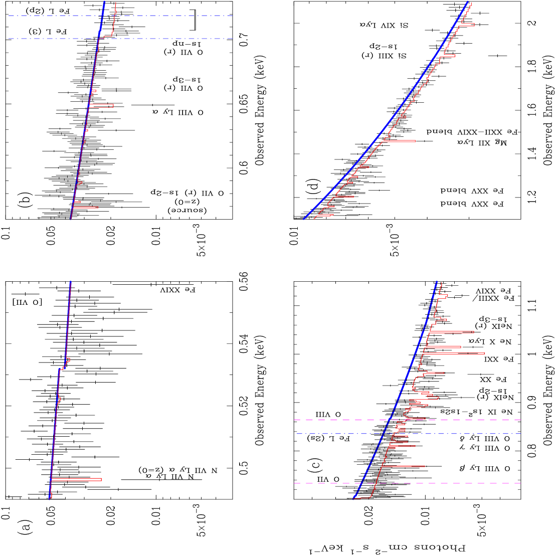
Figure 3:

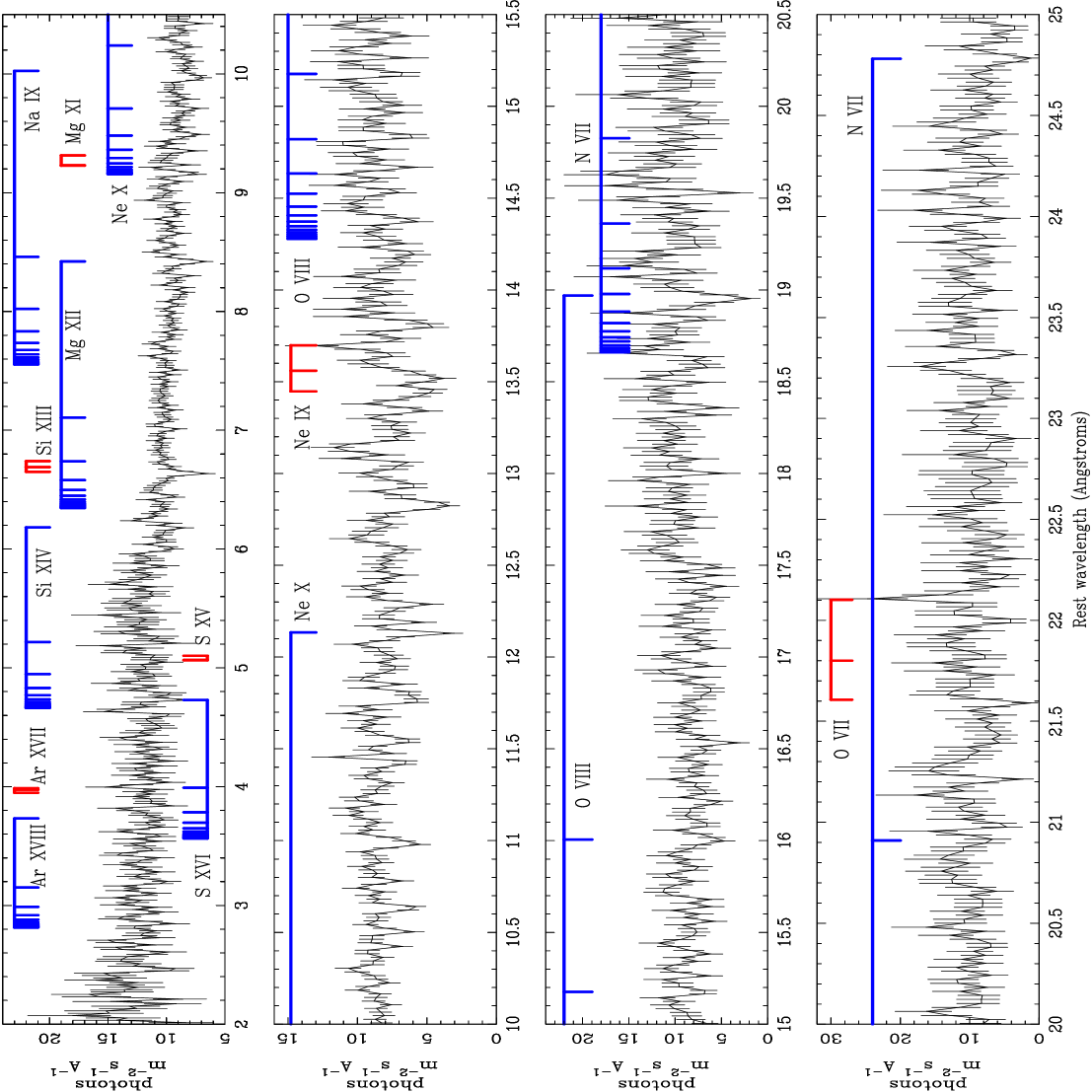
Figure 4:

Figure 5:

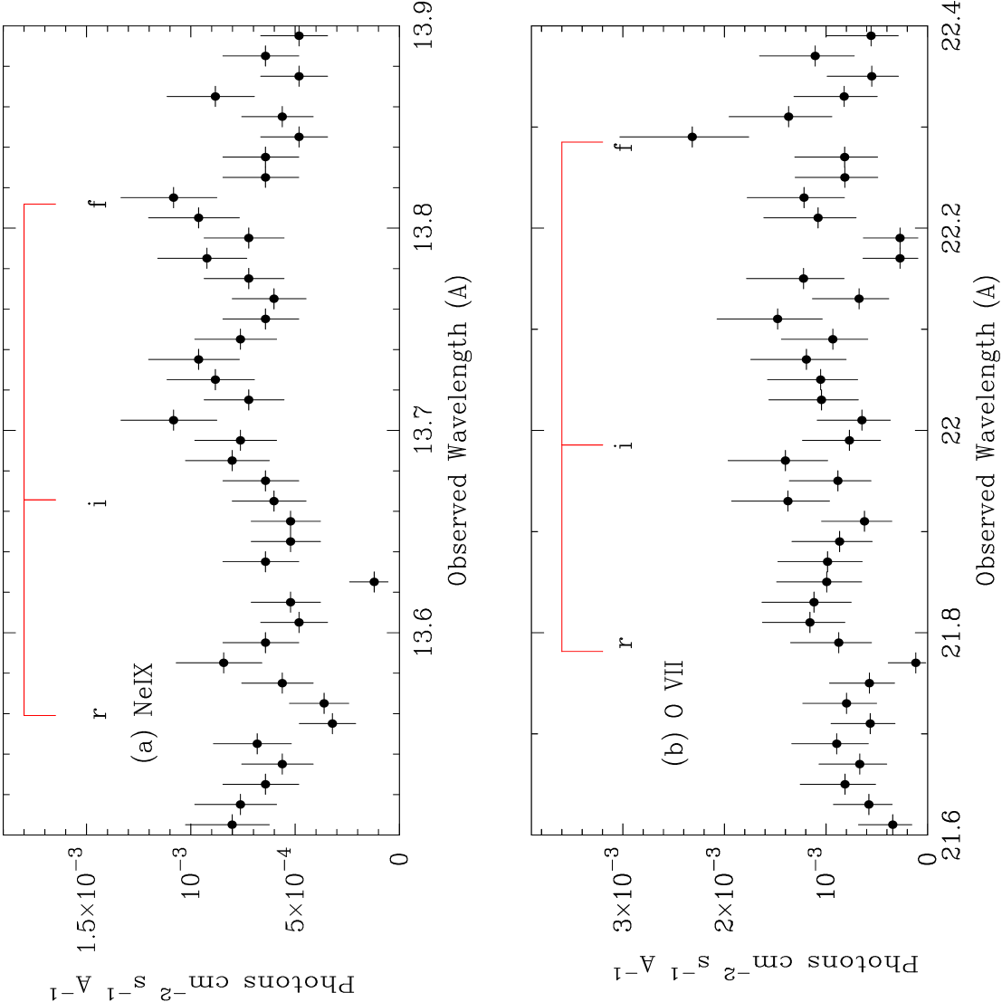
Figure 6:

Figure 7:

Figure 8:

Figure 9:

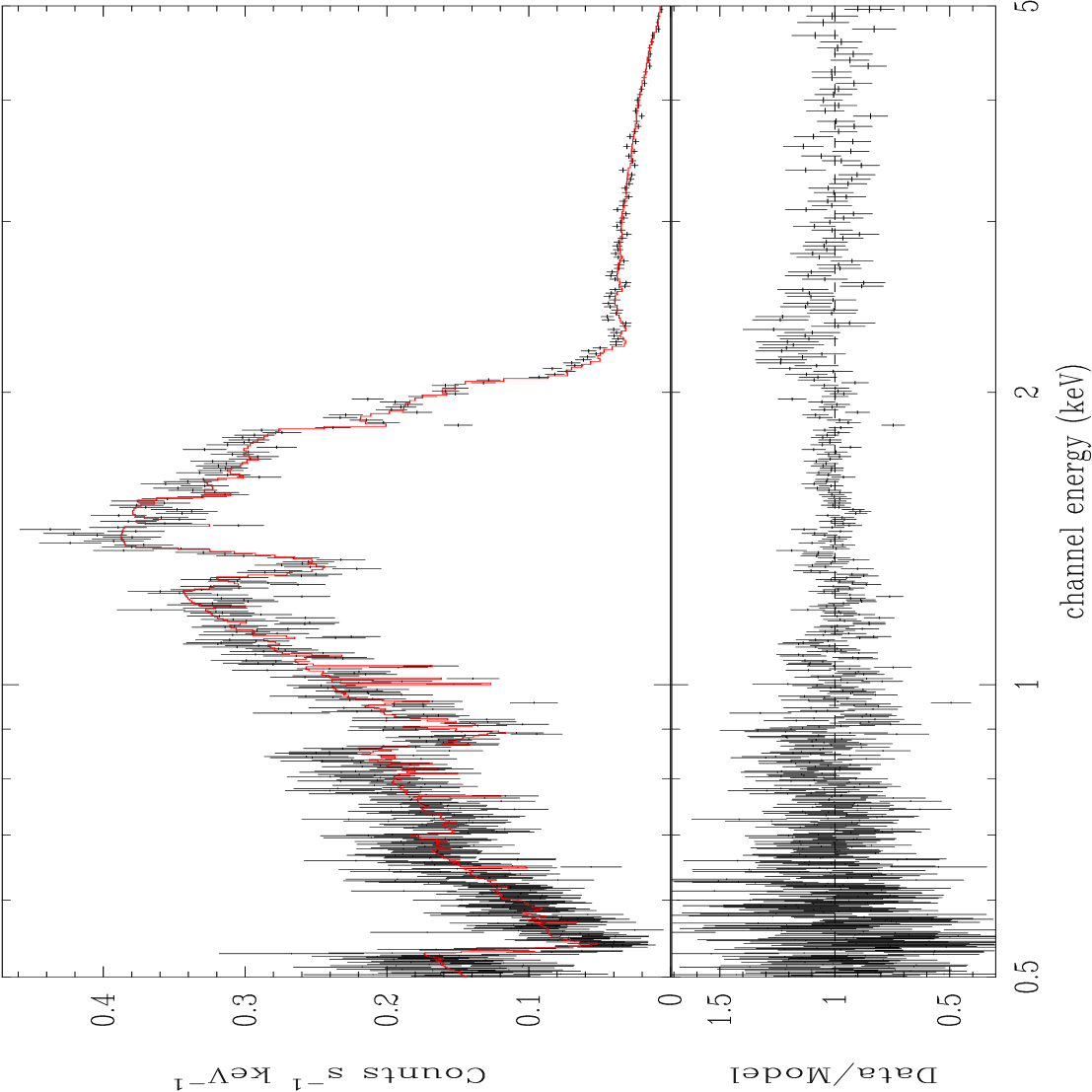
Figure 10:

Figure 11:

Figure 12:

Figure 13:

References

- Behar et al. (2001) Behar, E., Sako, M., & Kahn, S. M. 2001, ApJ, 563, 497
- Branduardi-Raymont et al. (2001) Branduardi-Raymont, G., Sako, M., Kahn, S. M., Brinkman, A. C., Kaastra, J. S., & Page, M. J. 2001, A&A, 365, 140
- Cash (1976) Cash, W., 1976, A&A, 52, 307
- De Vaucouleurs et al. (1991) De Vaucouleurs, G. et al. , 1991, 3rd Ref. Cat. of Bright Galaxies, v 3.9
- Elvis et al. (1989) Elvis, M., Wilkes, B. J., Lockman, F. J. 1989, AJ, 97, 777
- Fabian et al. (1989) Fabian, A. C., Rees, M. J., Stella, L., & White, N. E. 1989, MNRAS, 238, 729
- Gehrels (1986) Gehrels, N. 1986, ApJ, 303, 336
- George et al. (1998) George, I. M., Turner, T. J., Netzer, H., Nandra, K., Mushotzky, R. F., & Yaqoob, T. 1998, ApJS, 114, 73
- Gu et al. (2001) Gu, M. F., Kahn, S. M., Savin, D. W., Behar, E., Beiersdorfer, P., Brown, G. V., Liedahl, D. A., Reed, K. J., 2001, ApJ, 563, 462
- Guainazzi (1996) Guainazzi, M., Mihara, T., Otani, C., & Matsuoka, M. 1996, PASJ, 48, 781
- Kaastra & Steenbrugge (2001) Kaastra, J. S., Steenbrugge, K. C., 2001, in Conf. Proc., X-ray Emission from Accretion onto Black Holes, Proceedings, ed. T. Yaqoob, & J. H. Krolik (published electronically on ADS), E79 (astro-ph/0111419)
- Kaastra et al. (2002) Kaastra, J. S., Steenbrugge, K. C., Raassen, A. J. J., van der Meer R. L. J., Brinkman, A. C., Liedahl, D. A., Behar, E., & de Rosa, A. 2002, A&A, 386, 427
- Kaspi et al. (2002) Kaspi, S., et al. 2002, ApJ, 574, 643
- Lee et al. (2001) Lee, J. C., Ogle, P. M., Canizares, C. R., Marshall, H. L., Schulz, N. S., Morales, R., Fabian, A. C., & Iwasawa, K. 2001, ApJ, 554, L13
- Lee et al. (2002) Lee, J. C., Reynolds, C. S., Remillard, R., Schulz, N. S., Blackman, E. G., & Fabian, A. C. 2002, ApJ, 567, 1102
- Markert et al. (1995) Markert, T. H., Canizares, C. R., Dewey, D., McGuirk, M., Pak, C., & Shattenburg, M. L. 1995, Proc. SPIE, 2280, 168
- Matthews & Ferland (1987) Matthews, W. G., & Ferland, G. J. 1987, ApJ, 323, 456
- Mason et al. (2002) Mason, K. O. et al. 2002, ApJ, accepted (astro-ph/0209145)
- Nicastro et al. (2002) Nicastro, F. et al. 2002, ApJ, 573, 157
- Piro et al. (1997) Piro, L., Matt, G., & Ricci, R. 1997, A&A, 126, 525
- Piro et al. (1999) Piro, L., et al. 1999, ApJ, 514, L73
- Reynolds (1997) Reynolds, C. S. 1997, MNRAS, 286, 513
- Reynolds et al. (1997) Reynolds, C. S., Ward, M. J., Fabian, A. C., Celotti, A. 1997, MNRAS, 291, 403
- (24) Sako, M., et al. 2001a, A&A, submitted, 365, L168
- (25) Sako, M., et al. 2001b, ApJ, submitted (astro-ph/0112436)
- Turner et al. (2001) Turner, T. J., et al. 2001, ApJ, 548, L13
- Verner et al. (1996) Verner, D. A., Ferland, G. J., Korista, K. T. & Yakovlev, D. G. 1996, ApJ, 465, 487
- Ward et al. (1987) Ward, M., Elvis, M., Fabbiano, N., Carleton, P., Willner, S. P., & Lawrence, A. 1987, ApJ, 315, 74
- Weaver et al. (1998) Weaver, K. A., Krolik, J. H., & Pier, E. A. 1998, ApJ, 498, 213
- Yaqoob et al. (2003) Yaqoob, T., McKernan, B., Kraemer, S. B., Crenshaw, D. M., George, I. M., & Turner, T. J. 2003a, ApJ, 582, 105