The generality of inflation in closed cosmological models with some quintessence potentials

Abstract

We have investigated the generality of inflation (the probability of inflation in other words) in closed FRW models for a wide class of quintessence potentials. It is shown that inflation is not suppressed for most of them and for a wide enough range of their parameters. It allows us to decide inflation is common enough even in the case of closed Universe.

I Introduction

Recent observations of the supernovae type Ia snIa_1 ; snIa_2 combined with the CMB data CMB_rec and the data on large scale structure LSS_rec provide us with evidence our Universe is accelerating. One can explain it via a presence of the small positive $\Lambda$-term (cosmological constant). Here we have a deal with one of kinds of the dynamical $\Lambda$-term namely quintessence (see for review als_var00 ; var02 ; peeb_ratr02 ). It can explain the stage of inflation expansion infl and acceleration nowadays, this is the reason for improving interest for it recently. But the theories with the scalar field as a source of expansion have a free parameter – the potential of this scalar field. Yes, there were attempts to restore kind of the potential from SN Ia observations als-sn-v , but they did not give us an answer to our question about an exact kind of the potential. So one have a deal with different potentials of the scalar field in different areas of physics, not in the cosmology only. And the aim of this paper is the test of some of these potentials, attracted an attention recently. Namely we want to study the degree of inflationarity in Friedman-Robertson-Walker (FRW) models with different scalar field potentials motivated by particle physics, galaxies rotation curves, etc.

Saying the degree of inflationarity we mean the ratio of number of solutions experienced inflation to number of all possible ones. And saying about the number of solutions we mean not exact number – there is infinite number of all possible solutions – but the number one can obtain using evenly distributed net on the space of initial conditions. But choosing this net we are really choosing the measure on the initial conditions space and after doing it we can speak about the probability – very ratio is the probability of inflation for our model in the sense of measure we chose. So if this ratio is small enough for some potentials one can decide in the model with this potential the inflation is suppressed.

Here we work with closed models – curvature is the parameter which is ”forgotten” during inflation, but before inflation curvature had acted very strongly so presence of nonzero curvature will change the probability of inflation. By the way, recent CMB data CMB_rec show $\Omega_{0}=1.02\pm 0.02$ (but such a models – closed FRW – have some problems Linde_rec ) In the case of initially open or flat Universe the scale factor of the Universe $a$ cannot pass through extremum points. In this case all the trajectories starting from a sufficiently large initial value of the scalar field $\varphi_{0}$ reach a slow-roll regime and experience inflation. Here we call as trajectory the evolution curve of the Universe in some coordinates (for example ($a$,$t$) or as in we99 ($a$,$f$)). If we start from the Planck energy a measure of non-inflating trajectories for a scalar field with the mass $m$ is about $m/m_{P}$. From observational reasons, this ratio is about $10^{-5}$ so almost all trajectories lead to the inflationary regime. However, positive spatial curvature allows a trajectory to have a point of maximal expansion and results in increasing the measure of non-inflating trajectories (four ; B-Kh ).

The structure of the paper is following: first we write down main equations and introduce our measures. Then we have a deal with different potentials, motivated by observation and by particle physics and attracted an attention last years. For all of them we say some words about their origins with corresponding references and give the results for the degree of inflationarity in FRW models filled with the scalar field with these potentials.

II Main equations

Here we follow we01gr ; we01ijmpd . The equations describing the evolution of the Universe in closed FRW model are

$$\frac{m_{P}^{2}}{16\pi}\left(\ddot{a}+\frac{{\dot{a}}^{2}}{2a}+\frac{1}{2a}\right)+\frac{a}{4}\left(\frac{{\dot{\varphi}}^{2}}{2}-V(\varphi)\right)=0,$$

$$\ddot{\varphi}+\frac{3\dot{\varphi}\dot{\vphantom{\varphi}a}}{a}+\frac{dV(\varphi)}{d\varphi}=0,$$

and the first integral of the system is

$$\frac{3m_{P}^{2}}{8\pi}\left(\frac{\dot{a}^{2}}{a^{2}}+\frac{1}{a^{2}}\right)=\left(V(\varphi)+\frac{{\dot{\varphi}}^{2}}{2}\right).$$

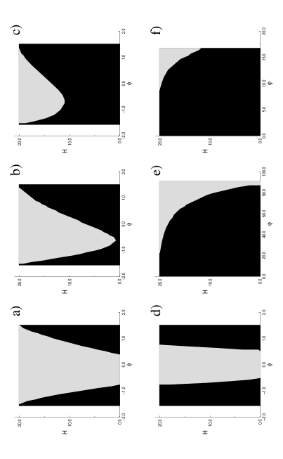
Figure 1: Examples of the areas on the initial conditions space which lead to inflation (grey dots) and don’t lead (black ones). Figs (a)–(c) correspond to the case of the inverse power-law potential, (d) – to the exponential potential and (e)–(f) – to the FCDM potential (see Sec. III F.) – field parametrization (see text for details).

Now we need to introduce parametrization – it determines the measure we use. For the FRW case the most common view of the trigonometrical (angular) parametrization $(\phi,H)$ is (*)

$$\frac{3m_{P}^{2}}{8\pi}\left(H^{2}+\frac{1}{a^{2}}\right)=m_{P}^{4},\quad H^{2}+\frac{1}{a^{2}}=\frac{8\pi m_{P}^{2}}{3},\quad H\in\left[0;\sqrt{\frac{8\pi}{3}}m_{P}\right);$$

$$V(\varphi)+\frac{{\dot{\varphi}}^{2}}{2}=m_{P}^{4},\quad V(\varphi)=m_{P}^{4}\cos^{2}\phi,\quad\frac{{\dot{\varphi}}^{2}}{2}=m_{P}^{4}\sin^{2}\phi,\quad\phi\in\left[-\frac{\pi}{2};\frac{\pi}{2}\right].$$

Here we have two dimensionless parameters: $\phi$ and the initial value of Hubble parameter $H$. This parametrization is very suitable for the potentials like power-law but unapplicable for example in the case of the complex scalar field we01gr ; we01ijmpd . In we01gr ; we01ijmpd we have introduced another parametrization – field one $(\varphi,H)$. It is determined as following – we will use initial value of the field $\varphi$ instead of $\phi$ and second coordinate is the same – initial value of the Hubble parameter $H$. This parametrization also have a disadvantage – it’s unapplicable for example for the runaway potentials.

Also we need to introduce the Planck boundary

$$V(\varphi)+\frac{{\dot{\varphi}}^{2}}{2}=m_{P}^{4}.$$

And our work is following: starting from the Planck boundary for given pair of the initial conditions ($(\phi,H)$ or $(\varphi,H)$) we numerically calculate further evolution of the Universe to get an answer – will our Universe experience inflation or not. Here we don’t check 60 e-foldings so when the scale factor increase in $10^{5}$ times, we call it as inflation (also we are checking for equation of state – during inflation the scalar field must violate the strong energy condition). And doing scans on all possible values of the initial conditions (with measure used we have bounded area of initial conditions) we get the ratio of the inflation solutions to all ones – the probability of inflation in some sense (one can use both the probability of inflation for the model with given potential and the degree of inflationarity of the model with given potential to call very ratio).

III Potentials

Before telling about the potentials we use, let us note – most of analysis’ given in references are made for the case of flat Universe. Well, we are living now in a flat (with good precision) Universe and so we have a deal with quintessence in flat Universe. But our Universe is flat due to the inflation and before inflation it could be curved. As we already noted above, here we have a deal with closed Universe.

In this paper we will use normalization $m_{P}^{2}/16\pi\equiv 1$ and one needs to keep it in mind while recalculating all values (like parameters in potentials, etc.) to more common quantities.

III.1 Power-law potentials

Figure 2: Inverse power-law potential: the dependence of the degree of inflationarity on the power $q$. I corresponds to the case $M~{}\sim~{}m_{P}$, II – $M~{}\sim~{}0.7~{}m_{P}$ and III – $M~{}\sim~{}0.4~{}m_{P}$.

Figure 3: Exponential potential: the dependence of the degree of inflationarity on $\lambda$. To recalculate $\lambda$ to more common values one needs to keep in mind $m_{P}^{2}/16\pi\equiv 1$.

Figure 4: ZWS potential: the dependence of the degree of inflationarity on $\alpha$ for $V_{0}~{}\sim~{}4~{}\times~{}10^{-4}~{}m_{P}^{4}$ (a) and $V_{0}~{}\sim~{}4~{}\times~{}10^{-2}~{}m_{P}^{4}$ (b). And like the case of the exponential potential while $\alpha$ is dimensional value $m_{P}^{2}/16\pi\equiv 1$.

Power-law potentials we99 are the potentials like

$$V(\varphi)=\frac{\lambda{\phi}^{n}}{n},\quad n\geq 2.$$

These potentials are well-studied and they lead to ”chaotic inflation” linde_ch . One can really use them as ”inflation part” in the potentials like ones considered by Peebles and Vilenkin peeb_vil_99 . Also they attract an attention for some their properties class ; Kolda_Lyth99 .

The degree of inflationarity for such potentials was studied in our previous papers we01gr ; we01ijmpd ; we_new , so here we will present results only. In the case $n=2$ we have about $47\%$ inflation solution in the case of field measure and about $63\%$ in the case of angular measure. Increasing $n$ will decrease the inflationarity in the case of field parametrization and will not change it for the angular parametrization (we_new ) – in the angular measure $63\%$ of all possible solutions experience inflation for $n=2,4,6,8$. And in the field measure we have about $30\%$ for $n=4$, $22\%$ for $n=6$ and $17\%$ for $n=8$. Damour-Mukhanov potential D-M behaves itself like power-law potentials in this sense and the probability of inflation is about $63\%$ in the case of the angular measure and not less then $47\%$ in the case of the field one (for discussion see we_new ).

III.2 Inverse power-law potentials

Pioneering studies of the inverse power-law potentials have been done by Ratra and Peebles peeb_ratr88 . These potentials are like ZWS

$$V(\phi)=M^{(4+q)}\varphi^{-q}.$$

Potentials of such a kind mostly studied for their scaling properties class and with some problems with quintessence Kolda_Lyth99 , but also they appear in some SUGRA theories as well Brax_Martin .

Here we examine potentials with large enough values of $M$ – really, for small ”observed” values peeb_vil_99 we obtained that inflationary solutions are not experience enough number of e-foldings. And it occurs just because of we have a deal with closed model – it naturally decrease number of inflationary solutions.

One of the ways to get large value of $M$ at the inflation stage and small one nowadays is to consider $M$ as not an exact constant but as slowly varing (namely decreasing). It would not change significantly during inflation but from inflation to nowadays can.

And the results are presented in Fig. 1: panels (a)–(c) represent examples of the initial condition space where grey point reflects initial condition leading to inflation (in the sense we noted above) and black one corresponds to recollapse. These figures are plotted for the case $M~{}\sim~{}m_{P}$ and $q=2$ (a), $q=6$ (b) and $q=8$ (c). In Fig. 2 we represent the final plot – with the degree of inflationarity on y axes and the power $q$ on x axes. There are three curves: I corresponds to the case $M~{}\sim~{}m_{P}$, II – $M~{}\sim 0.7~{}m_{P}$ and III – $M~{}\sim~{}0.4~{}m_{P}$. Note that in this case – inverse power-law potentials – we use angular measure only because in field measure the space of initial conditions is unbounded.

One can see from Fig. 1 (a)–(c) the areas are asymmetric with respect to $\phi=0$. It’s due to the parametrization – from (*) one can see that positive $\phi$ corresponds to positive $\dot{\varphi}$ so we start in this case ”down” the potential, at the same time negative $\phi$ corresponds to negative $\dot{\varphi}$ and so we start ”up” the potential. Namely due to this effect the area of inflationary solutions on the space of initial conditions is so asymmetric.

III.3 Exponential potential

Other interesting potential is an exponential one peeb_ratr88

$$V(\phi)=V_{0}\exp(-\lambda\varphi).$$

Potentials of such a kind naturally appear in high-energy physics in theories with Kaluza-Klein compactification, superstrings and supergravity theories exp_from_sugra and higher orders gravity theories exp_from_high_grav . This potential is also well-known in flat case for its tracker property and for some implications for observational cosmology ferr_joy98 ; exp_other ; class .

Our results are the same for a wide enough range of $V_{0}~{}\sim~{}m_{P}^{4}~{}\div~{}10^{-10}~{}m_{P}^{4}$. So we have only one free parameter – $\lambda$ and the results are plotted in Fig. 3. Example of the area on initial conditions space plotted in Fig. 1(d), where as in the previous cases black dot represents pair of initial $(\phi,H)$ not leading to inflation and grey dot represents leading one. Here as well as in the case of inverse power-law potentials we use only angular parametrization – the initial $\varphi$ is unbounded again.

III.4 ZWS potential

Figure 5: ULM potential: the dependence of the degree of inflationarity on $\alpha$ for fixed $V_{0}~{}=~{}4~{}\times~{}10^{-3}~{}m_{P}^{4}$ in panel (a) and for fixed $\lambda=0.7~{}m_{P}^{-1}$ in panel (b).

This potential

$$V(\varphi)=V_{0}\left[\exp\left(\frac{\alpha}{\varphi}\right)-1\right]$$

was suggested by Zlatev, Wang and Steinhardt ZWS while exploring scaling solutions, where $V_{0}$ and $\alpha$ are free parameters.

The dependence of the degree of inflationarity is plotted in Fig. 4: the case for $V_{0}~{}\sim~{}4~{}\times~{}10^{-4}~{}m_{P}^{4}$ in (a) panel and the case for $V_{0}~{}\sim~{}4~{}\times~{}10^{-2}~{}m_{P}^{4}$ in (b). Areas of initial conditions space leading and not to inflation look like ones in the case of inverse power-law potential (Fig. 1(a)–(c)). Due to the potential (runaway) we can use only the trigonometrical measure.

III.5 ULM potential

This potential was first considered by L.A. Ure$\tilde{\rm n}$a-López and T. Matos Matos_Urena-Lopez00 as a new cosmological tracker solution for quintessence. One can say it behaves itself like both exponential and inverse power-law potentials:

$$V(\varphi)=V_{0}\sinh^{-\alpha}(\lambda\varphi);$$

$$V(\varphi)=V_{0}(\lambda\varphi)^{-\alpha}\quad\mbox{for}\;|\lambda\varphi|<<1,$$

$$V(\varphi)=2^{\alpha}\,V_{0}e^{-\lambda\varphi\alpha}\quad\mbox{for}\;|\lambda\varphi|>>1$$

so its asymptotic behavior corresponds to an inverse power-law-like potential at early times and to an exponential one at later times.

The space of initial conditions is like the inverse power-law case (Fig. 1 (a)–(c)), and we have again only trigonometrical measure. The results for the degree of inflationarity are plotted in Fig. 5 with very degree on y axes and $\alpha$ on x axes. In this case we have two parameters – $V_{0}$ and $\lambda$ and it’s easily to understand the influence of them by fixing one of them and varying another one. Following its in (a) panel we fix $V_{0}~{}=~{}4~{}\times~{}10^{-3}~{}m_{P}^{4}$ and vary $\lambda$: $\lambda=0.7~{}m_{P}^{-1}$ (I), $\lambda=0.5~{}m_{P}^{-1}$ (II) and $\lambda=0.21~{}m_{P}^{-1}$ (III); in panel (b) we fix $\lambda=0.7~{}m_{P}^{-1}$ and vary $V_{0}$: $V_{0}~{}=~{}4~{}\times~{}10^{-2}~{}m_{P}^{4}$ (I), $V_{0}~{}=~{}4~{}\times~{}10^{-3}~{}m_{P}^{4}$ (II) and $V_{0}~{}=~{}4~{}\times~{}10^{-4}~{}m_{P}^{4}$ (III).

III.6 FCDM potential

This potential can describe both quintessence and new form of dark matter called sahni_wang_99 frustrated cold dark matter (FCDM) due to its ability to frustrate gravitation clustering at small scales. On this way it can help in solving some problems with dwarf galaxies halos halos .

Like previous one it have two asymptotic forms:

$$V(\varphi)=V_{0}(\cosh\lambda\varphi-1)^{p};$$

$$V(\varphi)\simeq\tilde{V}_{0}\,e^{p\lambda\varphi}\quad\mbox{for}\;|\lambda\varphi|>>1\;(\varphi>0),$$

$$V(\varphi)\simeq\tilde{V}_{0}(\lambda\varphi)^{2p}\quad\mbox{for}\;|\lambda\varphi|<<1,$$

where $\tilde{V}_{0}=V_{0}/2^{p}$.

Figure 6: FCDM potential: the dependence of the degree of inflationarity on $V_{0}$ and $\lambda$; (a)–(c) correspond to the case of field parametrization and (d)–(f) correspond to the case of trigonometrical parametrization. See text for detailed description of the panels.

In this case like in previous one we have two free parameters (while $p=0\div 1$): $V_{0}$ and $\lambda$. The space of initial conditions with the area of initial conditions leading to inflation looks like in the case of inverse power-law (see Fig. 1 (a)–(c)) in the trigonometrical parametrization case and for field parametrization (enjoy! for this potential we have field parametrization!) examples are presented in Fig. 1(e) and Fig. 1(f). And in Fig. 6 we have presented the dependence curves of the ratio of inflationary solutions to all possible ones on $p$ ($p\in[0,1]$). The dependence of the degree of inflationarity on both $V_{0}$ and $\lambda$ is hard to describe so we have presented the influence of $V_{0}$ and $\lambda$ on the curve when one of them is fixed and rest one is variable (as in the previous case). As we have noted above, in this case we have a deal with both field and angular measures. And one can see that the curves behave themselves differently in these measures.

Very results are presented in Fig. 6: panels (a)–(c) correspond to the case of field parametrization and panels (d)–(f) correspond to the case of trigonometrical parametrization. Let us describe them: in Fig. 6(a) and 6(d) there are dependence curves of the degree of inflationarity on $\lambda$ for $V_{0}=4\times 10^{-7}m_{P}$ and curves are: $\lambda=0.7m_{P}^{-1}$ (I), $\lambda=7m_{P}^{-1}$ (II) and $\lambda=30m_{P}^{-1}$ (III). In Fig 6(b) and 6(e) we again fixed $V_{0}=4\times 10^{-4}m_{P}$ and $\lambda=0.7m_{P}^{-1}$ (I), $\lambda=7m_{P}^{-1}$ (II) and $\lambda=30m_{P}^{-1}$ (III). To understand the influence of $V_{0}$ on the dependence curve one can compare these two cases as well as use Figs. 6(c) and 6(f), where we fixed $\lambda=7m_{P}^{-1}$ and curves are $V_{0}=4\times 10^{-4}m_{P}$ (I), $V_{0}=4\times 10^{-7}m_{P}$ (II) and $V_{0}=4\times 10^{-10}m_{P}$ (III). One can see that in the limit of small $V_{0}$ all dependence curves are similair each other.

So from Fig. 6 (a)–(f) one can determine values for $\lambda$ and $V_{0}$ which correspond to large enough degree of inflationarity.

IV Summary and discussions

In this paper we have investigated a wide class of the quintessence potentials from the point of view of the generality of inflation. Some of these potentials are motivated via particle physics (for review see, for example, Lyth_Riotto99 ) and most of them were also studied recently from the point of view of scaling or tracker solutions. So here we have made some tests of them – are they able to provide our Universe with inflation? And in this way we obtained the answer – yes, closed FRW models filled with the scalar field with these potentials experience inflation for a wide enough range of their parameters. So inflation is general for a wide enough class of the cosmological models.

As we have a deal with closed model, the degree of inflationarity is smaller then in flat (and of course open) case – at the early stage of the Universe’s evolution the scale factor was small so presence of nonzero curvature might change the situation significantly. But we have seen that even in the case of positive spatial curvature potentials we have considered behave itself well from this point of view and the inflation is not suppressed in models filled with the scalar field with these potentials. The inflation in closed models was recently studied in the case of pure $\Lambda$-term lambda and they also have a result that the inflation doesn’t suppress.

In this paper we used as determination of inflation the situation when the scale factor increases in $10^{5}$ times (about 12 e-foldings) and this approximation works well. For some cases we have checked its up to $10^{25}$ (about 57 e-foldings) and the results are the same with precision about $0.04\%$. So our approximation works well.

V Acknowledgments

We wish to thank N. Savchenko and A. Toporensky for useful discussion.

References

- (1) S.J. Perlmutter et. al., Nature (London) 391, 51 (1998); S.J. Perlmutter et. al., Astrophys. J. 517, 565 (1999).
- (2) A.G. Riess et. al., Astron. J. 116, 1009 (1998).
- (3) A. Benoit et al., astro-ph/0210306; J.E. Ruhl et al., astro-ph/0212229; J.H. Goldstein et al., astro-ph/0212517; D.N. Spergel et al., astro-ph/0302209.
- (4) M. Colless et al., Mon. Not. R. Astron. Soc. 328, 1039 (2001); Efslathiou et al., Mon. Not. R. Astron. Soc. 330, L29 (2002); Verde et al., Mon. Not. R. Astron. Soc. 335, 432 (2002).
- (5) V. Sahni and A. Starobinsky, Int. J. Mod. Phys. D 9, 373 (2000) [astro-ph/9904398].
- (6) V. Sahni, Class. Quant. Grav. 19, 3435 (2002) [astro-ph/0202076].
- (7) P.J.E. Peebles and B. Ratra, Rev. Mod. Phys. (to be published), astro-ph/0207347.
- (8) A.H. Guth, Phys. Rev. D 23, 347 (1981); A.D. Linde, Phys. Lett. B 108, 389 (1982); A. Albrecht and P.J. Steinhardt, Phys. Rev. Lett. 48, 1220 (1982); Sato, Mon. Not. R. Astron. Soc. 195, 467 (1981); A. Starobinsky, Pis’ma A.J. 4, 155 (1978), Sov. Astron. Lett. 4, 82 (1978).
- (9) A. Starobinsky et. al., Phys. Rev. Lett. 85, 2236 (2000); 85, 1162 (2000); A. Starobinsky, JETP Lett. 68, 757 (1998).
- (10) A. Linde, astro-ph/0303245.
- (11) V.A. Belinsky, L.P. Grishchuk, Ya.B. Zeldovich and I.M. Khalatnikov, JETP 89, 346 (1985).
- (12) V.A. Belinsky and I.M. Khalatnikov, JETP 93, 784 (1987); V.A. Belinsky, H. Ishihara, I.M. Khalatnikov and H. Sato, Prog. Theor. Phys. 79, 676 (1988).
- (13) S.A. Pavluchenko and A.V. Toporensky, Gravitation Cosmology 6, 241 (2000) [gr-qc/9911039].
- (14) S.A. Pavluchenko and A.V. Toporensky, Gravitation Cosmology Suppl. 8, 168 (2002).
- (15) S.A. Pavluchenko, N.Yu. Savchenko and A.V. Toporensky, Int. J. Mod. Phys. D 11, 805 (2002) [gr-qc/0111077].
- (16) S.A. Pavluchenko and A.V. Toporensky, in preparation.
- (17) D.H. Lyth and A. Riotto, Phys. Rept. 314, 1 (1999) [hep-ph/9807278].
- (18) T. Damour and V.F. Mukhanov, Phys. Rev. Lett. 80, 3440 (1998), A. Liddle and A.Mazumdar, Phys. Rev. D 58, 083508 (1998).
- (19) A.R. Liddle and R.J. Scherrer, Phys. Rev. D 59, 023509 (1998).
- (20) B. Ratra and P.J.E. Peebles, Phys. Rev. D 37, 3406 (1988); P.J.E. Peebles and B. Ratra, Astrophys. J., Lett. Ed. 325, L17 (1988).
- (21) A. Linde, Phys. Lett. B 129, 177 (1983).
- (22) P.J.E. Peebles and A. Vilenkin, Phys. Rev. D 59, 063505 (1999).
- (23) V. Sahni and L. Wang, Phys. Rev. D 62, 103517 (2000) [astro-ph/9910097].
- (24) B. Moore et. al., astro-ph/9903164; J.F. Navarro and M. Steinmetz, astro-ph/9908114; S. Ghigna et. al., astro-ph/9910166; D.N. Spergel and P.J. Steinhardt, Phys. Rev. Lett. 84, 3760 (2000); M. Kanionkowski and A.R. Liddle, Phys. Rev. Lett. 84, 4525 (2000).
- (25) P.G. Ferreira and M. Joyce, Phys. Rev. Lett. 79, 4740 (1997); Phys. Rev. D 58, 023503 (1998).
- (26) C. Kolda and D.H. Lyth, Phys. Lett. B 458, 197 (1999).
- (27) Ph. Brax and J. Martin, Phys. Lett. B 468, 40 (1999) [astro-ph/9905040]; Phys. Rev. D 61, 103502 (2000).
- (28) C. Wetterich, Nucl. Phys. B252, 302 (1985); B252, 688 (1985); Astron. Astrophys. 301, 321 (1995); E.J. Copeland et. al., Ann. N.Y. Acad. Sci. 688, 647 (1993).
- (29) C. Wetterich, Nucl. Phys. B252, 309 (1985); Q. Shafi and C. Wetterich, Phys. Lett. B 152, 51 (1985); Nucl. Phys. B289 787 (1987); J. Halliwell, Nucl. Phys. B266, 228 (1986); J.D. Barrow and S. Cotsakis, Phys. Lett. B 214, 515 (1988).
- (30) A.B. Burd and J.D. Barrow, Nucl. Phys. B308, 929 (1988); J. Yokoyama and K. Maeda, Phys. Lett. B 207, 31 (1988); P. Binétruy, Phys. Rev. D 60, 063502 (1999) [hep-ph/9810553].
- (31) E.J. Copeland, A.R. Liddle and D. Wands, Phys. Rev. D 57, 4686 (1998); P.T.P. Viana and A.R. Liddle, Phys. Rev. D 57, 674 (1998); T. Barreiro, E.J. Copeland and N.J. Nunes, Phys. Rev. D 61, 127301 (2000); A. Albrecht and C. Skordis, Phys. Rev. Lett. 84, 2076 (2000).
- (32) I. Zlatev, L. Wang and P.J. Stainhardt, Phys. Rev. Lett 82, 896 (1999); Phys. Rev. D 59, 123504 (1999).
- (33) L.A. Urea-López and T. Matos, Phys. Rev. D 62, 081302(R) (2000).
- (34) J.P. Uzan, U. Kirchner and G.F.R. Ellis, [astro-ph/0302597].