Cosmic Evolution Impressions on Lensing Maps

Abstract

I investigate through simulations the redshift dependence of several lensing measures for two cosmological models, a flat universe with a cosmological constant ($\Lambda$CDM), and an open universe (OCDM). I argue that quintessence models can be seen as an intermediate model between these two models under the weak gravitational lensing perspective. I calculate for the convergence field the angular power spectrum, the variance and higher order moments, the probability distribution function, and the Minkowski functionals. I find that in the redshift range examined (from $z=0.7$ to $z=3$ various statistics show an increase of the non-Gaussianity of the lensing maps for closer sources. Lensing surveys of higher redshift are expected to be less non-Gaussian than shallow ones because of the non-linear evolution of the density field, and the central limit theorem.

Department of Physics, University of Durham, South Road, Durham DH1 3LE

1. Introduction

A lensed image contains information about the positions of the lens and source object, and about the lens itself (e.g. its refractive index). In the cosmological context the mass inhomogeneities in the universe act as gravitational lenses to source objects far away. The dominant cosmological picture today describes a universe that is expanding and has growing density perturbations. The exact characterization and quantification of these phenomena are essential pursuits of observational Cosmology, and their description by a theoretical model is a major objective for cosmologists.

Weak gravitational lensing studies can contribute to this enterprise because lensing maps depend on the evolution of the large-scale structure and on the geometrical properties of the universe (the cosmological expansion).

In this section I briefly review some of the formalism of cosmic expansion and structure formation, and point how these two aspects of cosmic evolution are captured by weak gravitational lensing maps.

1.1. Cosmological Geometry

In a Friedmann-Robertson-Walker model, assuming isotropy and homogeneity, the geometry of the universe can be described by the metric

$$d\tau^{2}=dt^{2}-a^{2}(t)\left[dr^{2}+f_{K}^{2}(r)d\phi^{2}\right]\;,$$ (1)

where $t$, $r$ and $\phi$ are the comoving coordinates, and $f_{K}$ is the curvature-dependent comoving angular distance ($=r$ for a flat universe, $=\sinh r$ for open, and $=\sin r$ for closed). The expansion factor $a(t)$ is determined by the equation

$$\dot{a}^{2}-\frac{8\pi G}{3}\rho a^{2}=-k\;,$$ (2)

in a universe of curvature $k$ ($=0,-1,1$ in the case that it is flat, open, or closed, respectively), and of density $\rho$. In terms of the density parameters $\Omega_{\Lambda}$, $\Omega_{m}$ and $\Omega_{r}$, for a cosmological constant, matter, and radiation, respectively,

$$\rho=\frac{3H^{2}_{o}}{8\pi G}\left(\Omega_{\Lambda}+\Omega_{m}a^{-3}+\Omega_{r}a^{-4}\right)\;.$$ (3)

It is also useful to define the Hubble parameter

$$H \equiv \frac{\dot{a}}{a}\;,$$ (4)

$$H(a) = H_{o}\left[\Omega_{\Lambda}(1-a^{-2})+\Omega_{m}(a^{-3}-a^{-2})+a^{-2}\right]^{1/2}\;,$$ (5)

and to remember the relation $a=1/(z+1)$.

In a quintessence model the cosmological constant is substituted by a dark energy component, which has negative pressure, i.e. a negative $w_{Q}$ in its equation of state $p_{Q}=w_{Q}\rho_{Q}$. In the case in which $w_{Q}$ is constant the Hubble expansion rate is them

$$H(a)=H_{o}\left[\Omega_{\Lambda}(a^{-3(w_{Q}+1)}-a^{-2})+\Omega_{m}(a^{-3}-a^{-2})+a^{-2}\right]^{1/2}\;,$$ (6)

which reduces to the cosmological constant case [equation (5)] when $w_{Q}=-1$.

1.2. Density Perturbations

The current standard explanation for the existence of a large-scale structure in the matter distribution in the universe is that initial small fluctuations in a remote past evolved (grew) due to gravitational attraction. That is the gravitational instability scenario. The origin and characteristics of the initial inhomogeneities is subject of great interest for Cosmology and fundamental Physics, but will not be discussed here.

The matter distribution can be described by the density contrast $\delta=\rho/\bar{\rho}-1$, where $\bar{\rho}$ is the average density, and its evolution in the linear regime is given by

$$\ddot{\delta}+2\frac{\dot{a}}{a}\dot{\delta}=4\pi G\bar{\rho}\,\delta$$ (7)

The growing mode solution for this equation can be factored into spatial and temporal functions

$$\delta({\bf x},t)=D(t)\,\delta({\bf x},t_{o}),$$ (8)

where the growth function is

$$D(a)\propto\frac{\dot{a}}{a}\int_{0}^{a}\frac{1}{\dot{a}}da\;$$ (9)

which can be approximated, apart from a normalization factor, by (Carroll, Press & Turner 1992; Lahav et al. 1991)

$$D(a)\approx a\frac{5}{2}\Omega_{m}(a)\left\{\Omega_{m}^{4/7}(a)-\Omega_{\Lambda}(a)\left[\frac{1}{2}+\left(1+\frac{\Omega_{m}(a)}{2}\right)\left(1+\frac{\Omega_{\Lambda}}{70}(a)\right)\right]\right\}^{-1}\,,$$ (10)

$$\Omega_{m}(a)=\frac{\Omega_{m}}{a^{3}}\left(\frac{H_{0}}{H}\right)^{2}\,,$$ (11)

$$\Omega_{\Lambda}(a)={\Omega_{\Lambda}}\left(\frac{H_{0}}{H}\right)^{2}\,.$$ (12)

The growth function must be normalized such that $D(a=1)=1$. For an Einstein-de Sitter Universe there is no suppression of gravitational clustering, and the growth function reduces to the scale factor, $D(a)=a$.

For a quintessence model (Ma et al. 1999) $\Omega_{m}(a)=\Omega_{m}/[\Omega_{m}+(1-\Omega_{m})a^{-3w_{Q}}]$, and the growth factor can be approximated by (apart from a normalization factor)

$$D_{Q}(a) \approx (-w_{Q})^{t}a\frac{5}{2}\Omega_{m}(a)$$

$$\times \left\{\Omega_{m}^{4/7}(a)-1+\Omega_{m}(a)+\left[1+\frac{\Omega_{m}(a)}{2}\right]\left[1+\frac{1-\Omega_{m}(a)}{70}\right]\right\}^{-1}\;,$$

$$t=-(0.255+0.305w_{Q}+\frac{0.0027}{w_{Q}})[1-\Omega_{m}(a)]-(0.366+0.266w_{Q}-\frac{0.07}{w_{Q}})\ln{\Omega_{m}(a)}\;.$$ (14)

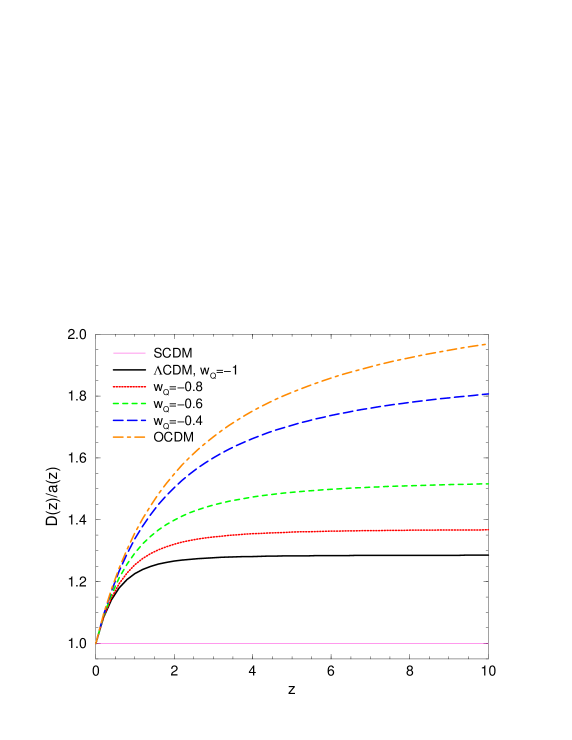
Figure 1.: Linear growth of factor. SCDM has $\Omega_{m}=1$, all other models have $\Omega_{m}=0.3$, $w_{Q}$ is the equation-of-state coefficient for a quintessence field model with $\Omega_{Q}=0.7$.

I use the expressions (1.2.) and (10), properly normalized, to plot the curves in Figure 1 that show the linear growth factor for several cosmological models. Note that the effect of a quintessence description for the dark energy component is equivalent to an intermediate suppression of growth between a flat universe with cosmological constant and an open universe.

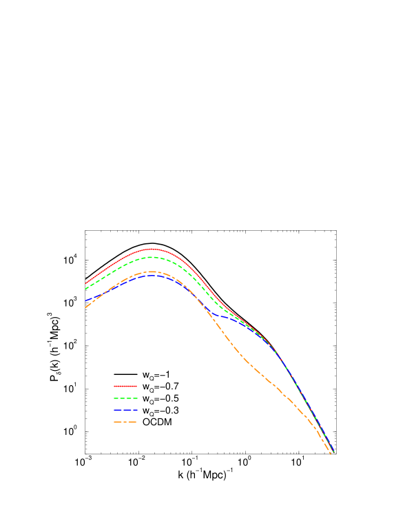
Figure 2.: Power spectrum of matter density fluctuations. All models (quintessence models and OCDM) were normalized to match the density anisotropies observed in the cosmic background radiation (Bun & White 1997 and Ma et al. 1999). The case $w_{Q}=-1$ is equivalent to a $\Lambda$CDM model.

The power spectrum of the matter density perturbation is a powerful statistical descriptor of the large-scale structure of the universe. From linear theory (which is valid at the largest scales) the power can be written as

$$P(k,a)=Ak^{n}T^{2}(k)D^{2}(a)\;,$$ (15)

where $A$ is a normalization, $n$ is the initial power spectrum index, and $T(k)$ is the transfer function, which modifies a initial power-law spectrum of density perturbations, building in information about the energy components of the universe. However, linear theory becomes a bad approximation when $\delta({\bf x},t)\gg 1$, which happens at small scales at late stages of the evolution of the density fields. The non-linear evolution causes the power spectrum at large wavenumber $k$ to be underestimated by linear theory. The corrected calculation of the density field evolution in the non-linear regime requires the use of N-body simulations. From that one can obtain approximations for the non-linear power spectrum using prescriptions such the ones developed by Hamilton et al. (1991), and Scranton & Dodelson (2000). See figure 2 for plots of the non-linear power spectrum of quintessence models with various equation-of-state coefficients, and of an open universe, with no dark energy.

1.3. Weak Lensing Dependence on Cosmological Evolution

The distortion matrix from which the shear and the convergence fields are defined is explicitly dependent on the cosmic evolution from the redshift of the source $z_{s}$ until today ($z=0$)

$${\cal A}_{ij}({\mbox{\boldmath$\theta$}},z_{s})=-2\int_{0}^{z_{s}}{g(z,z_{s})\partial_{i}\partial_{j}\Phi({\mbox{\boldmath$\theta$}},z)dz}\;.$$ (16)

This expression integrates the evolution in the geometry of the universe, which is encoded in the factor $g$, and the evolution of the gravitational potential $\Phi$.

For the convergence this dependence is represented thought the comoving distance

$$w(a)=\int_{a}^{1}{\displaystyle\frac{da^{\prime}}{a^{\prime 2}H(a^{\prime})/H_{0}}}\;,$$ (17)

in the expression

$$\kappa({\mbox{\boldmath$\theta$}},z_{s})=\frac{3H_{o}^{2}}{2}\Omega_{m}\int_{0}^{w_{s}}{\frac{g(w^{\prime},w_{s})}{a(w^{\prime})}\delta({\mbox{\boldmath$\theta$}},w^{\prime})dw^{\prime}}\;,$$ (18)

where

$$g(w^{\prime},w)=\frac{f_{K}(w^{\prime})f_{K}(w-w^{\prime})}{f_{K}(w)}\;.$$ (19)

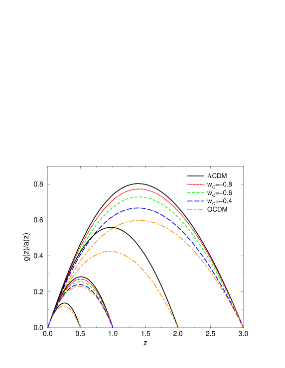
Figure 3.: Geometrical weighting of density perturbations in weak lensing. Lines labeled by $w_{Q}$ represent quintessence models with such equation-of-state coefficient.

Figure 3 shows the geometrical weighting of the density fluctuations for a source at a redshift $z$ given by the factor $g/a$ at equation (18). The maximum contribution for lensing comes from structures with redshifts close to half of the source redshift. Quintessence models have an intermediate weighting between a $\Lambda$CDM and a OCDM model, and the farther the source the more significant is the difference between the models.

2. Lens Evolution

In this section I use a set of statistics to characterize the evolution of the matter density field, or more properly, the evolution of lens-planes. I analyze the projected density contrast field of boxes of 100 $h^{-1}Mpc$ of side that evolve in time. The simulations use $128^{3}$ dark-matter particles (no baryonic matter) in two models, $\Lambda$CDM and OCDM.

Figure 4 shows the evolution of the two-dimensional power spectrum of the lenses, and illustrates the growth of structure in the matter density field. It is possible to note that small-scale structures (represented by large $k$) have a stronger increase than large-scale structures (small $k$), as is expected from non-linear evolution. The difference between $\Lambda$CDM and OCDM is more notable at large redshifts, because the simulations were normalized to the cluster abundance today.

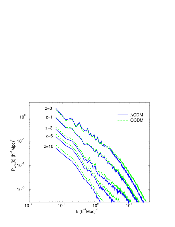
Figure 4.: 2D power spectrum of lens-planes.

The growth of structure in time can be also appreciated by the increase of the field variance, skewness, and kurtosis - see Figure 5. These two last quantities quantify the growth of non-Gaussianities in the density field, which in this case is originally Gaussian, due to non-linear evolution. The same information can be obtained from the PDF (figure 6).

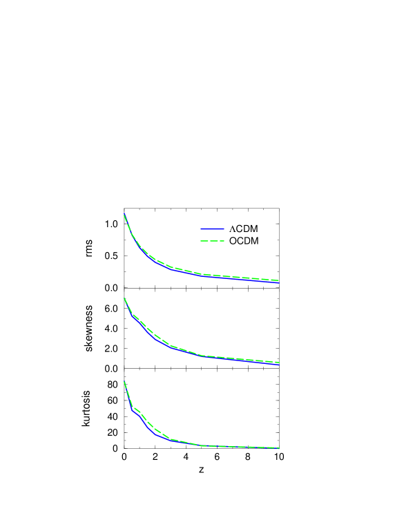
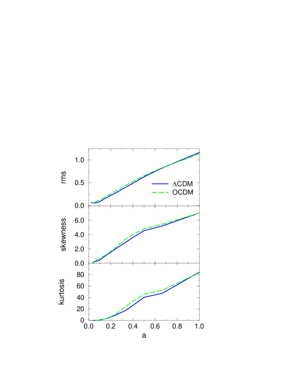
Figure 5.: The rms, skewness, and kurtosis of the projected density contrast field as redshift (left) and scale factor (right) functions for $\Lambda$CDM (solid lines) and OCDM (dashed lines). Projected boxes have 100 1h^-1Mpc, and were smoothed at 1 1h^-1Mpc scale.

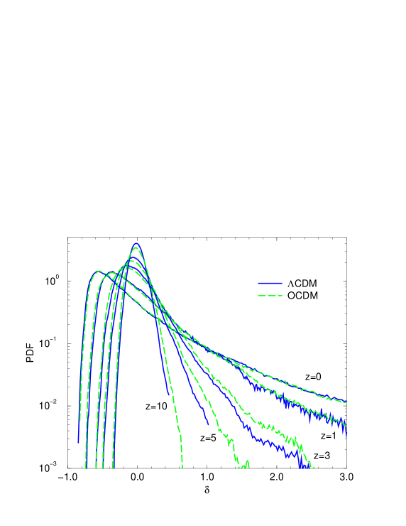
Figure 6.: Probability distribution function for the density contrast of lens planes with 1h^-1Mpc smoothing.

The last aspect of the density field to be analyzed is its morphology. I use the second (contour length) and third (genus) Minkowski functionals parameterized by the first functional (fractional area) to characterize the morphology of the lens-planes. Figure 7 shows that up to a redshift z=5 there is little change in these two functionals. The third functional is not symmetric in relation to the midpoint along the axes of the plot, which again shows the non-Gaussianity of the density field. Both models are almost indistinguishable from one another under this statistics. The meaning of these observations is that in both models the non-trivial morphology, i.e. the morphology distinct from that of a Gaussian field, emerges at earlier times than z=5, and that in the late universe the morphology of the LSS as described by the Minkowski functionals evolves little if the functionals are parameterized by the fractional area, making them independent of the PDF.

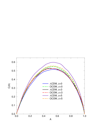
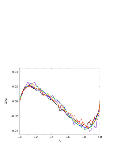
Figure 7.: Minkowski functionals parameterized by the fractional area $A$ for the density contrast of lens-planes.

3. Redshift Dependence of Lensing Measures

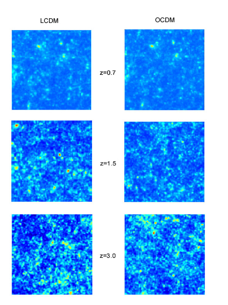
Figure 8.: Convergence maps for $\Lambda$CDM (left) and OCDM (right) for source plane at redshifts 0.7, 1.5 and 3 (top to bottom). All maps are 1.7$\times$1.7 degrees², are smoothed with a 1 arcmin top-hat radius, and use the same color scale (from deep blue for the minimum value to red to the maximum value)

I generated simulated convergence maps using the multiple-plan lens method (see Guimarães, 2002 for more details) for $\Lambda$CDM and OCDM. I used the Hydra N-body code (Couchman, Thomas & Pearce, 1995) to evolve 128³ particles from a redshift $z=50$ to $z=0$, simulating the large-scale mass distribution in the two models. For the $\Lambda$CDM ($\Omega_{m}=0.3,\Omega_{\Lambda}=0.7$) simulation I adopt a cluster normalization equivalent to $\sigma_{8}=0.9$, and a simulation box of 141.3 $h^{-1}Mpc$. For the OCDM ($\Omega_{m}=0.3,\Omega_{\Lambda}=0.7$) simulation I adopt a cluster normalization equivalent to $\sigma_{8}=0.84$, and a simulation box of 128 $h^{-1}Mpc$. A Hubble parameter $h=0.7$ was used in both simulations.

Another examined model mimics an universe with the geometry of the $\Lambda$CDM model but no structure evolution. In this toy-model the structre at any redshift has the same statistical properties that today.

Figure 8 shows a realization of the convergence map for both models with a source plane at three redshifts. The redshift dependence is very clear, but the differentiation between $\Lambda$CDM and OCDM is less evident. A quantitative characterization of the models requires the use of several statistics applied to many realizations of the lensing maps. I calculate as a function of source redshift the following statistics for the convergence: the angular power spectrum, the rms (root mean square), the skewness ($S=\langle{\kappa^{3}}\rangle/\sigma_{\kappa}^{3}$), the kurtosis $(K=(\langle{\kappa^{4}}\rangle/\sigma_{\kappa}^{4})-3$), the probability distribution function, and the Minkowski functionals. The results shown in the figures are the result of 20 realizations of the convergence map for each model, and for each redshift. The variance of the measures are shown only for $\Lambda$CDM and serves as a reference for maps of same size of other models. The sizes of the used maps are (side of square), 4.6^∘ for $z=0.7$, 3.5^∘ for $z=1$, 2.5^∘ for $z=1.5$, 2.2^∘ for $z=2$, and 1.8^∘ for $z=3$.

Figure 9 shows the results for the angular power spectrum of the convergence field. There is an overall increase of the spectrum amplitude as the redshift of the source increases. This is also reflected in the rms plot (Figure 10), since the field variance is proportional to the convergence angular power spectrum. The same figure shows a decreasing skewness and kurtosis for larger redshifts. These two statistics can be considered measures of the non-Gaussianity of the field since for a Gaussian field they are zero.

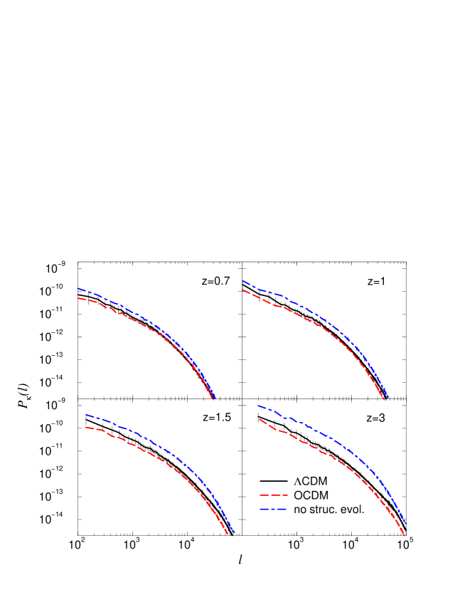
Figure 9.: Angular power spectrum of the convergence field for $\Lambda$CDM (left) and OCDM (right) for source plane at redshifts 3, 2, 1.5, 1, 0.7 (top to bottom curves). No smoothing was used.

A power law fit to the rms results yield the following redshift dependence for the shear variance

$$\langle{\gamma^{2}}\rangle=\langle{\kappa^{2}}\rangle\propto z^{\alpha}\;,$$ (20)

where $\alpha=1.34\pm 0.08$ for OCDM, and $\alpha=1.5\pm 0.1$ for $\Lambda$CDM. This later result coincides with the value obtained by Jain & Seljak (1997), $\alpha=1.52$, but is lower than the value obtained by Barber (2002), $\alpha=2.07\pm 0.04$.

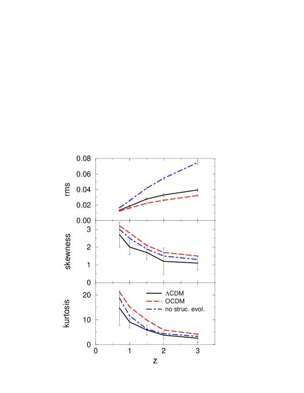
Figure 10.: The rms, skewness, and kurtosis of the convergence field as redshift functions for $\Lambda$CDM (solid lines) and OCDM (dashed lines). Maps were smoothed at 1 arcmin scale.

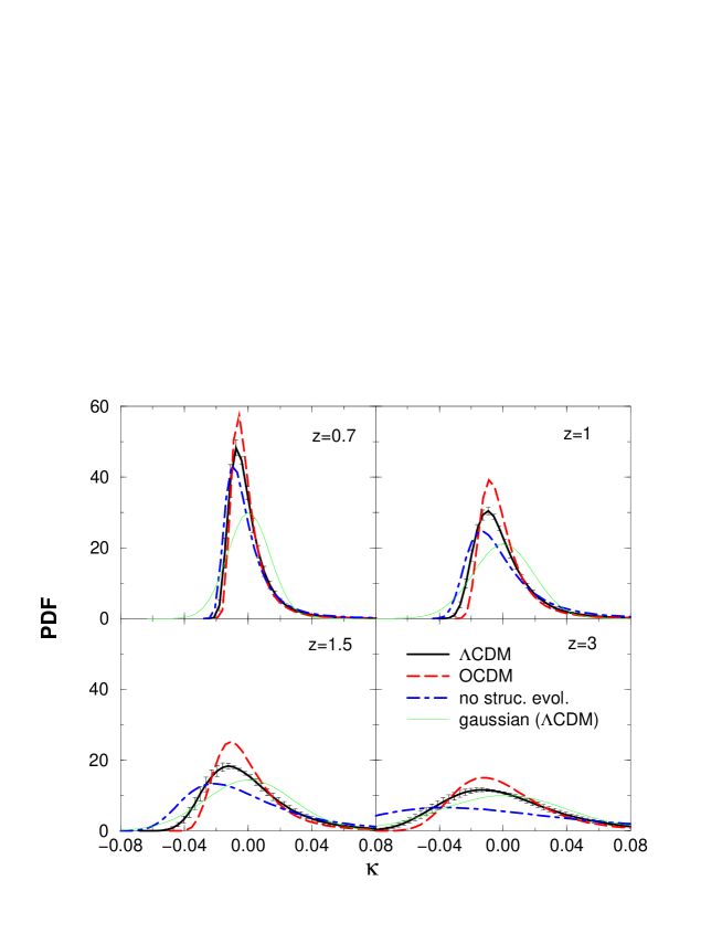
Figure 11.: Probability distribution function of the convergence field smoothed at 1 arcmin scale. The dashed lines are the PDF of the Gaussianized fields.

Departures from Gaussianity can also be observed in the probability distribution function of the lensing maps – figure 11. I plot the PDF for the Gaussianized $\Lambda$CDM maps to show more clearly the non-Gaussianity of the maps. The convergence fields were Gaussianized by expanding them in Fourier modes, and reconstructing the fields with the same mode amplitudes, but random mode phases.

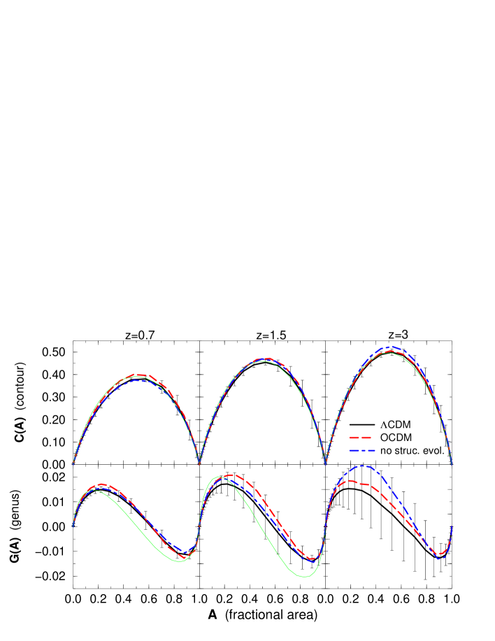
Figure 12.: Minkowski functionals parameterized by the fractional area $A$ of the convergence field smoothed at 1 arcmin scale. The thin lines are for the Gaussianized maps.

Figure 12 shows the results for the second and third Minkowski functionals (contour length and topological genus, respectively), parameterized by the first functional (fractional area). I choose not to present the first Minkowski functional because it does not carry any extra information in relation to the PDF. The parameterization by the fractional area $A$ instead of the map threshold $\nu=\kappa/\sigma_{\kappa}$ is aimed to further decouple the information contained in the Minkowski functionals from the PDF. The results for the Gaussianized fields compared with the original field results show that the third functional $G(A)$ puts in evidence the non-Gaussianity of the maps much more clearly than the second functional $C(A)$. Note that the third functional does not show a clear redshift dependence under the conditions examined.

4. Conclusion

In this paper I have made predictions for the redshift evolution of statistical measures of weak lensing maps. These predictions show a relatively small difference between OCDM and $\Lambda$CDM models with adiabatic Gaussian initial conditions, and will thus also hold in quintessence models in similar conditions. Given the robustness of the results in redshift dependence within the class of models tested, I propose the study of the redshift dependence of weak gravitational lensing as a test for the stability of our current paradigm for the formation of galactic structure by gravitational instability in a theory with a primordial scale invariant spectrum of Gaussian perturbations.

This work concentrates on the convergence field, which can be seen as a weighted projection of the density contrast field until the source. The characteristics of the lensing map will them be dependent not only on the density field, but on how it is weighted. I show how these two components relate to the cosmic evolution, and what are the resulting lensing properties for two cosmological models.

The differentiation of the lens-planes is small for the two models considered when the spectrum of matter fluctuations is normalized to match the abundance of rich clusters today. However the lensing geometrical factor, the term $g/a$, is clearly distinct between the two models, allowing the clear differentiation of the models by a power spectrum analysis, or by one-point statistics. It is to be expected, therefore, that for quintessence models these statistics will assume values intermediate between what was obtained for $\Lambda$CDM and OCDM, because the geometrical factor is intermediate.

It would be very useful if the most popular N-body codes, for example Hydra (which was used here), could incorporate quintessence models. That would allow a direct calculation of lensing measures in this model.

The morphological analysis of the maps indicates some evolution of the second Minkowski functional (equal) for both models, and no distinguishable evolution of the third functional (genus) in the redshift range explored. The third functional is a better indicator of the departure from Gaussianity than the second functional. Because the third Minkowski functional depends weakly on the redshift of the source it is a specially recommended statistic to evaluate Gaussianity in surveys that have a poor redshift determination of the sources.

References

Barber A.J., 2002, astro-ph/0108273

Bun E.F., White M. 1997, ApJ, 480, 6

Carroll S.M., Press W.H., Turner E.L. 1992, ARA&A, 30, 499

Couchman H.M.P., Thomas P.A., Pearce F.R. 1995, ApJ, 452, 797

Guimarães A.C.C. 2002, MNRAS, 337, 631

Hamilton A.J.S., Kumar P., Lu E., Matthews A. 1991, ApJ, 374, L1

Jain B., Seljak U., White S. 2000, ApJ, 530, 547

Ma C.-P., Caldwell R.R., Bode P., Wang L. 1999, ApJ, 521, L1

Scranton R., Dodelson S. 2000, preprint (astro-ph/0003034)