Infrared Parallaxes for Methane T dwarfs

Abstract

We report final results from our 2.5 year infrared parallax program carried out with the European Southern Observatory 3.5m New Technology Telescope and the SOFI infrared camera. Our program targeted precision astrometric observations of ten T type brown dwarfs in the J band. Full astrometric solutions (including trigonometric parallaxes) for nine T dwarfs are provided along with proper motion solutions for a further object. We find that HgCdTe-based infrared cameras are capable of delivering precision differential astrometry. For T dwarfs, infrared observations are to be greatly preferred over the optical, both because they are so much brighter in the infrared, and because their prominent methane absorptions lead to similar effective wavelengths through the J-filter for both target and reference stars, which in turn results in a dramatic reduction in differential colour refraction effects. We describe a technique for robust bias estimation and linearity correction with the SOFI camera, along with an upper limit to the astrometric distortion of the SOFI optical train. Colour-magnitude and spectral-type-magnitude diagrams for both L and T dwarfs are presented which show complex and significant structure, with major import for luminosity function and mass function work on T dwarfs. Based on the width of the early L dwarf and late T dwarf colour magnitude diagrams, we conclude the brightening of early T dwarfs in the J passband (the “early T hump”) is not an age effect, but due to the complexity of brown dwarf cooling curves. Finally, empirical estimates of the “turn on” magnitudes for methane absorption in field T dwarfs and in young stars clusters are provided. These make the interpretation of the T6 dwarf $\sigma$ Ori J053810.1-023626 as a $\sigma$ Ori member problematic.

1 Introduction – Methane T-type Brown Dwarfs

Numerous examples of the field counterparts to the extremely cool methane brown dwarf Gl 229B (Nakajima et al., 1995) are now known (Strauss et al., 1999; Burgasser et al., 1999, 2000a, 2000b; Leggett et al., 2000; Tsvetanov et al., 2000; Cuby et al., 2000). These objects are now uniformly classified as “T dwarfs” (Burgasser et al., 2002b; Geballe et al., 2002), and have such low photospheric temperatures (800-1300K), that their photospheres are dominated by the effects of dust and methane formation (Allard et al., 2001), neither of which are amenable to simple modeling. The discovery of sizable numbers of T dwarfs, means that we are now in a position to use direct trigonometric parallax observations to empirically determine the loci of T dwarf cooling curves, rather than relying on models. The discovery of several T dwarfs by SDSS with spectra bridging the L and T spectral types (e.g. Leggett et al. 2002; Geballe et al. 2002) means we are also in a position to empirically determine where on these brown dwarf cooling curves the L-T transition occurs.

Trigonometric parallaxes are also essential to understanding the space density of T dwarfs. Luminosity function estimates for T dwarfs (eg. Burgasser 2002a) are currently based on limited parallaxes and assumptions about object binarity. (Recent programs targeting more L and T dwarfs (Martıǹ, Brander & Basri, 1999; Koerner et al., 1999; Reid et al., 2001; Burgasser et al., 2003a; Close et al., 2003), indicate that $\sim$10-20% of objects observed in sufficient detail are found to be binary.) Luminosity functions based on currently available colour-magnitude relations will therefore be problematic at best. Trigonometric parallaxes are therefore required to determine the actual luminosities of these objects and indicate whether they are single or binary, so that more meaningful luminosity functions for T dwarfs can be constructed.

2 Parallaxes and the Infrared

Traditional parallax techniques based on photography are completely unable to target objects as faint and red as T dwarfs. CCD parallax work in the optical at the USNO, ESO and Palomar (Monet et al., 1992; Dahn et al., 2002; Tinney, 1996; Tinney et al., 1995; Tinney, 1993) have shown that parallaxes can be obtained for objects as faint as I=18-19 at distances $\lesssim$70 pc. However, this still leaves the T dwarf class of objects (with I$\gtrsim$21) unobservable. To date only a few of the very brightest and closest T dwarfs have proved tractable for CCD parallax work (Dahn et al., 2002).

Over the last two years, therefore, we have been extending optical CCD astrometric techniques into the infrared, where the J$<$16 magnitudes of most of the detected T dwarfs make significant progress possible. Indeed, there are several reasons to prefer the infrared for high precision astrometry. First, the effects of differential colour refraction (the different amount of refraction the atmosphere produces in red target stars, compared to blue reference stars, see Monet et al. 1992) are reduced by working at longer wavelengths. Second, because T dwarfs suffer methane absorption at the red end of their J- and H-band spectra, their effective wavelengths through a J- or H-filter are much closer to that of a typical background reference star, than is the case in the optical. These effects combined mean that the stringent requirements on maintaining control of observations at constant hour angles (at least for T dwarfs) is not present in the infrared (cf. Section 6.1). This considerably increases the flexibility and efficiency of infrared parallax observing, over the optical. Third, seeing improves in the infrared, leading to smaller images, smaller amounts of differential seeing, and so higher astrometric precision. And finally, T dwarfs show much greater contrast to sky in the near-infrared than in the optical.

Infrared parallax observations have been pioneered by Jones (2000), who targeted the extremely active (and unfortunately at 76 pc also quite distant) late M dwarf PC0025+0447, as well as the nearby M dwarf VB10. The USNO also has an infrared astrometric program in operation, from which published results are expected shortly (Vrba et al., 2002).

3 Observations & Sample

Observations were carried out at 7 epochs over the period 2000 April 17 to 2002 May 30. At each epoch, observations were carried out on either two half- or two full-nights. All observations were obtained with the SOFI infrared camera on the European Southern Observatory (ESO) 3.5m New Technology Telescope (NTT). SOFI was used in its “large field” mode in which it provides a 4.92′$\times$4.92′ field-of-view with 0.28826″ pixels (cf. Section 4.2).

Exposures of each target were acquired with a fixed dither pattern (Fig. 2) as eight 120s exposures though the SOFI J filter. The exposure pattern was designed so that this 16 minutes of dithered exposure time sampled many different inter-pixel spacings. As much as was feasible (given observing time constraints) we attempted to acquire all epoch observations at the same hour angle as the very first epoch observation acquired, so as to minimise DCR effects. Each epoch observation was also carried out with a specified reference star positioned within a few pixels of its position when observed on the very first epoch. This ensures all observations are carried out as near differentially as possible.

Seeing conditions over the course of this program varied. Figure 1 shows a histogram of the seeing full-width at half maxmimum for all our astrometric observations. The median seeing was 0.82″, with 80% of data being acquired in seeing conditions between 0.55 and 1.25″.

In addition to these epoch observations, all targets were also observed as they rose and set, so that DCR calibrations for each target could be developed, following the technique described in Tinney et al. (1995); Tinney (1996). The J filter was chosen for these observations as it offers the best contrast between sky- and T dwarf brightness. Typical near-infrared sky colours at La Silla are J–H=1.7, H–K=1.0-2.0 (2.0 for dark, 1.0 for bright) (ESO SOFI on-line documentation). By contrast typical T dwarf colours are -0.5$<$J–H$<$0.5 and H–K$<$0.5 (Burgasser et al., 2002b), which means most T dwarfs are around a magnitude brighter compared to the sky in J, than they are in H or K.

The sample of objects observed is listed in Table 1, along with indications as to which targets were observed at which epochs. SOFI has a nominal gain of 5.6e-/adu, and a nominal read-noise of 14e- per exposure.

Table 1: NTT Infrared Parallax Target Sample.

Object	Position	Apr	Jul	Mar	Apr	Jul	Mar	May	Ref.
	(J2000)	‘00	‘00	‘01	‘01	‘01	‘02	‘02
2MASS J05591914-1404488 (catalog )	05h59m19$\fs$1$-$14°04′49″	x			x		x
SDSS J10210969-0304201 (catalog )	10h21m09$\fs$7$-$03°04′20″		x	x	x	x	x
2MASS J10475385+2124234 (catalog )	10h47m53$\fs$8$+$21°24′23″	x	x	x	x		x
2MASS J12171110-0311131 (catalog )	12h17m11$\fs$1$-$03°11′13″	x	x	x	x	x	x
2MASS J12255432-2739466AB (catalog )	12h25m54$\fs$3$-$27°39′47″	x	x	x	x	x	x
SDSS J12545390-0122474 (catalog )	12h54m53$\fs$9$-$01°22′47″		x	x		x	x
SDSS J13464645-0031504 (catalog )	13h46m46$\fs$4$-$00°31′50″	x	x	x	x	x	x
2MASS J15344984-2952274AB (catalog )	15h34m49$\fs$8$-$29°52′27″	x	x	x	x	x	x
2MASS J15462718-3325111 (catalog )	15h46m27$\fs$2$-$33°25′11″	x	x	x	x	x	x
SDSS J16241437+0029156 (catalog )	16h24m14$\fs$4$+$00°29′16″	x	x	x	x	x	x

Figure 1: Seeing histogram for all observations in this program.

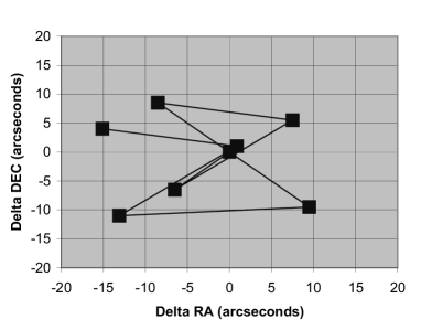
Figure 2: Fixed dither pattern used for all epoch observations. Offsets are in arcseconds from the initial base pointing position.

3.1 Object Names

With the exception of $\epsilon$ Ind B (Scholz et al., 2003), all the objects discussed in this paper have been discovered by either the 2MASS (www.ipac.caltech.edu/2mass), SDSS (www.sdss.org) or DENIS (cdsweb.u-strasbg.fr/denis.html) sky surveys, and have been given object names by those surveys, based on their positions in J2000 coordinates. These names have the advantage of being very specific and informative, and the disadvantage of being lengthy and clumsy. Throughout this paper, therefore, we will generally give an object’s complete name when it is first used, and thereafter refer to it (when not confusing to do so) by a shortened 2Mhhmm, SDhhmm or Dhhmm form where hh and mm are the right ascension hour and minute components of its name.

4 Analysis

The analysis adopted for these data falls into two main areas: processing to produce linearised, flattened and sky subtracted images, which was quite specific to the SOFI instrument; and astrometric processing of these images, which identically follows that described in Tinney (1993); Tinney et al. (1995); Tinney (1996).

4.1 Processing SOFI data

Dark frames and zero-points : Dark frames obtained with SOFI reveal significant structure, which can be broken down into a few components.

1. a significant ($\sim$50-100 adu peak-to-peak) vertical structure, known as the “shade”, which varies in intensity and shape with the overall level of illumination of the array;

2. a small (1-20 adu) dark current from the instrument and a small readout amplifier glow in each quadrant; and

3. a tiny ($<$1 adu) but fixed “ray” pattern left after the previous two are modeled and removed from dark current data.

The shade pattern is of most concern as the remaining fixed patterns are small compared to the sky brightness. Figure 3 shows a dark current image displaying the shade effect, together with a set of vertical medianned profiles through the shade. Unfortunately, this shade profile is not constant - it varies with the intensity of the overall level of illumination of the array during an exposure, meaning one has an unknown zero-point for every pixel in every exposure.

Calibration of the shade was achieved as follows. A small aperture (used to mask the instrument entrance when observing with one of the smaller fields of view) was inserted into the NTT focal plane, and a series of flat fields obtained with varying exposure times. Because only the central quarter of the array is illuminated by this procedure, it is possible to extract a shade profile from the edge of each image. It is also possible to record the level of illumination of the array which produced that shade profile. By performing a least-squares cubic polynomial fit through each pixel of these shade profiles (which correspond to rows on the detector) as a function of array illumination, it is possible to develop a parametrization for the shade profile. Using this parametrization it is a simple matter to produce a shade profile estimate for each data image, and subtract it. The result is an image with zero-point constant across the array.

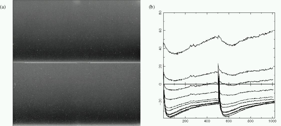
Figure 3: (a) Example of the SOFI shade pattern in a dark frame. (b) SOFI shade profiles obtained as vertical cuts through dark regions of the partially illuminated detector, for a range of count rates in the illuminated regions of the detector. The profiles span count rates in adu/pix from top to bottom of 3199, 2221, 1861, 1467, 1086, 958 701, 685, 554, 483, 226 and 87.

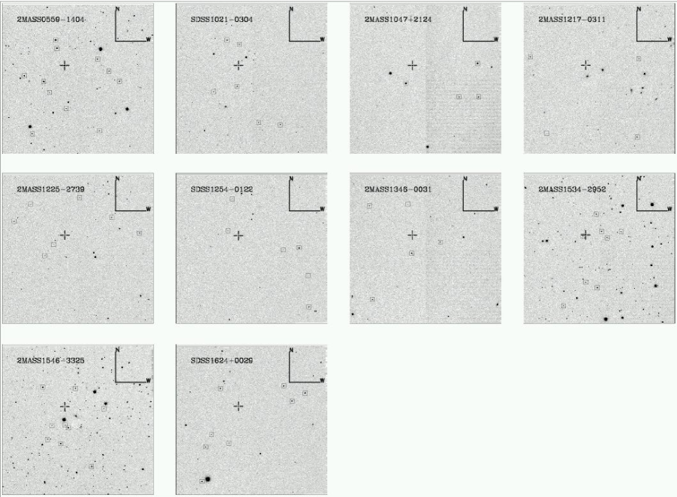
Figure 4: J-band finding charts with our target T dwarfs (cross hairs), and astrometric reference stars (boxes) highlighted. Each field is 295.2″ on a side. The direction bars in each field are 1′ in size.

Linearity : All infrared detectors are non-linear to some extent. For SOFI, ESO usually recommends keeping sky and target object intensities below 10,000 adu in order to maintain linearity at better than 1%. Unfortunately, such an observing strategy is not useful for astrometry, which demands the largest possible dynamic range to ensure targets (and reference stars) of widely differing magnitudes are usable in widely varying seeing conditions. We therefore calibrated the linearity of SOFI using the same shade profile data obtained above. Once the data have been shade corrected, they can then be used to examine the response of each pixel to a constant light source over widely varying exposure times. Repetition of a ’calibration’ exposure time throughout the sequence allows the lamp’s constancy to be calibrated – usually to within $\pm$ 0.5%. A sample of the resulting linearity correction is shown in Fig. 5 for one of the SOFI quadrants. In all cases these tests were performed independently for each quadrant, and the results were always consistent with the same linearity correction for all quadrants. A single correction was therefore derived as the mean of those in each quadrant. Fig. 5 shows that the detector is $\approx$2.5% non-linear at 20,000adu above bias, but that data can be obtained and linearity corrected even up to 25,000adu.

Figure 5: A linearity fit for a single SOFI quadrant. The data points plotted are the counts a perfectly linear detector would see, divided by the observed counts, as a function of observed counts. The fit is a fourth order polynomial, which models the amount of non-linearity as a function of observed counts. The actual linearity correction coefficients used are given in the text.

To linearise a pixel, then, with raw intensity $I_{ij}$, it is simply necessary to multiply it by the polynomial P($I_{ij}$) = $a_{0}+a_{1}\,I_{ij}+a_{2}\,I_{ij}^{2}+a_{3}\,I_{ij}^{3}$. The coefficients adopted were $a_{0}=1.0,a_{1}=0.0,a_{2}=1.11329\times 10^{-10},a_{3}=-2.46799\times 10^{-15}$ for 2000 April - 2001 April, and $a_{0}=1.0,a_{1}=0.0,a_{2}=8.6124661\times 10^{-11},a_{3}=-1.6986849\times 10^{-15}$ for 2001 July - 2002 May.

Inter-quadrant Row Crosstalk : HgCdTe detectors typically show an effect known as inter-quadrant row crosstalk (Finger & Nicolini, 1998). This has the effect that a constant, small fraction of the total flux seen in each row is seen as crosstalk at the same row in all the other quadrants. Correction of this effect is straightforward. The detector is integrated up into a single vertical column, then the two halves of this cut (Y=1-512 and Y=513-1024) are averaged, multiplied by a single cross-talk constant, and subtracted from every column of the detector. We found a crosstalk coefficient of 2.8$\times$10^-5 worked well.

Flat-fielding : Flat-fielding was performed using dome flats. Because of the (variable) shade pattern present in every dome flat, NTT staff have developed an observing recipe to obtain a “special” flat-field without a shade pattern present. Or one can used the shade calibration procedure described above to correct standard dome-flat fields. Both were tried for this program and both provided similar results. In the end every run’s data was flattened with a “special” dome flat, as per usual for SOFI observing.

Sky subtraction : Each group of eight 120s dithered exposures was then used to create a normalised and medianned sky frame, which was re-normalised to each of the twelve observations to perform sky subtraction. So that the data frames would maintain approximate photon-counting errors, an appropriate constant sky level was then added back in to each frame

Astrometric processing : Following this processing then, we have eight bias-subtracted, linearised, cross-talk corrected, flattened and sky-subtracted data frames for each astrometric epoch. These were then subject to further processing (ie. object finding and point-spread function fitting using DAOPHOT, DCR calibration and proper-motion and parallax solution fitting) as eight individual observations, in a manner identical to that described in Tinney (1993); Tinney et al. (1995); Tinney (1996).

4.2 Astrometric Calibration of SOFI

Astrometric calibration observations were acquired in USNO Astrometric Calibration Region M (Stone et al., 1999) on 2001 July 12 and 13. These consisted of sixteen 60s exposures (on each night) scattered throughout the 3.2°$\times$7.6° region which Stone et al. (1999) have astrometrically calibrated. These were processed identically to our main astrometric targets. Reference catalogue positions were extracted from the USNO ACR catalogue in SOFI-field-sized regions around each nominal telescope pointing position. These positions were then tangent projected (using the SLALIB library Wallace 1999) to provide reference data sets in arcsecond offsets on the sky for each observation. These were matched against the observed data to derive a set of linear (ie shift, scale and rotate) transformations from the SOFI pixel positions to arcsecond offsets on the sky. These transformations determine the SOFI plate scale on this night to be 0.28826$\pm$0.00003″/pixel, and that the detector pixel’s misalignment with N-S (0.030$\pm$0.003°). These data were also analysed to examine the amount of astrometric distortion (ie. variability in the instrument plate scale with position in the field) present in the SOFI optical train. The astrometric calibration data show there is no significant astrometric distortion in the SOFI Large Field optics. The plate scale in the field corners is the same as that in the field center to within 0.1%. The SOFI field can be considered astrometrically flat to 0.1%.

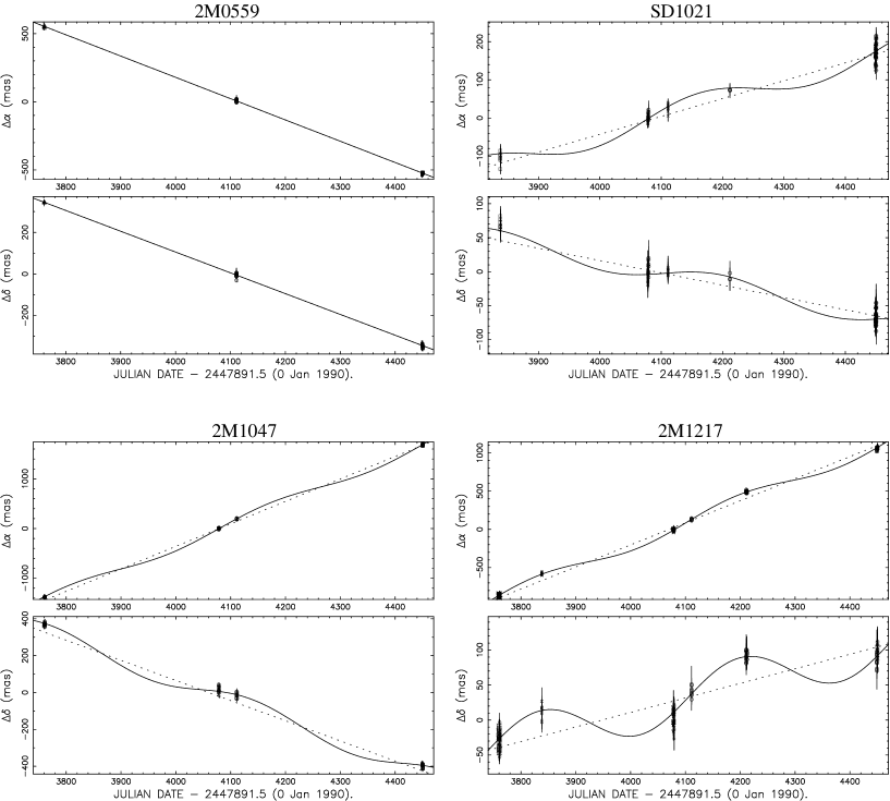
Figure 6: Plots of the observed astrometric motions of our target T dwarfs, relative to the ensemble of selected background reference stars. For each object we show plots of their motion in right ascension ($\Delta\alpha$) and declination($\Delta\delta$) as a function of date. Also shown are the fitted proper motion + parallax (solid lines) and where a significant parallax has been measured, the fitted proper motion alone (dotted lines). The parameters fitted are given in Table 2.

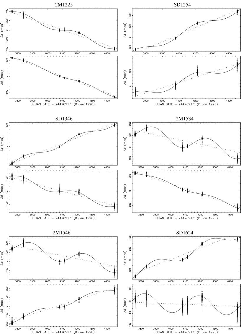
Figure 6 (cont.):

Table 2: NTT Infrared Parallax Sample - Relative Astrometry

Object	Nf,n,s	$\pi_{r}$	$\mu_{r}$	$\theta_{r}$	Vtan
		(mas)	(mas)	(°)	(km/s)
2M0559	71,5,11	(96.9)	677.4$\pm$2.5	122.6$\pm$0.1	33.1$\pm$0.1
S1021	112,7,6	34.4$\pm$4.6	183.2$\pm$3.4	248.8$\pm$1.0	25.2$\pm$2.4
2M1047	70,7,4	110.8$\pm$6.6	1698.9$\pm$2.5	256.4$\pm$0.1	72.7$\pm$4.4
2M1217	143,10,4	90.8$\pm$2.2	1057.1$\pm$1.7	274.1$\pm$0.1	55.2$\pm$1.4
2M1225AB	128,12,7	75.1$\pm$2.5	736.8$\pm$2.9	148.5$\pm$0.1	46.5$\pm$1.7
S1254	104,7,6	73.2$\pm$1.9	491.0$\pm$2.5	284.7$\pm$0.1	31.8$\pm$1.0
2M1346	118,9,5	68.3$\pm$2.3	516.0$\pm$3.3	257.2$\pm$0.2	35.8$\pm$1.4
2M1534AB	140,11,8	73.6$\pm$1.2	268.8$\pm$1.9	159.1$\pm$0.1	17.3$\pm$0.4
2M1546	150,10,9	88.0$\pm$1.9	225.4$\pm$2.2	32.5$\pm$0.6	12.1$\pm$0.4
S1624	152,11,8	90.9$\pm$1.2	373.0$\pm$1.6	268.6$\pm$0.3	19.5$\pm$0.3

5 Results for T dwarfs

Astrometric solutions for our T dwarf targets were evaluated in a manner identical to that used by Tinney et al. (1995). Briefly the procedure is to transform (using a linear transformation with rotation and a scale factor) all the frames for a given object, onto a chosen master frame of good seeing (known to have the detector rows and columns aligned with the cardinal directions to within $\pm 0.1$°), using a set of well exposed reference stars which were required to appear in every frame; differential colour refraction (DCR – see Tinney et al. (1995)) coefficients were then evaluated for each of these reference stars (relative to the unknown ‘mean’ DCR coefficient for the reference star set), and the reference frame corrected for DCR; each frame was then re-transformed onto the ‘master’ frame; the DCR coefficient for the program object (relative to the DCR-corrected reference frame) was then evaluated; the program object was DCR corrected; and finally, an astrometric solution in parallax and proper motion was made independently for both the $\alpha$ and $\delta$ directions, using a linear weighted-least-squares fit. Uncertainties arising from the DCR correction and the residuals about the reference frame transformation for each frame were carried through to this solution fit, so observations taken in poor seeing or with poor signal-to-noise due to cloud autmoatically receive low weight. The final parallax was taken to be the weighted mean of the $\alpha$ and $\delta$ solutions. Finding charts for our target stars (taken from our SOFI data) showing both the target and reference stars adopted can be seen in Fig. 4.

The resulting relative astrometry is presented in Table 2, the columns of which show; the number of frames (N_f), nights (N_n) and reference stars (N_s) used in each solution; the parallax and proper motion solutions (relative to the background reference stars chosen); and the derived tangential velocity for each target )based on the measured parallax, except for 2MASS0559, for which we adopt the distance of Dahn et al. 2002). Plots of these fits are shown in Fig. 6. The reference stars used to obtain this relative astrometry are typically within $\pm$1 mag. of the apparent magnitude of our target T dwarf. At these magnitudes (J=15-18) the reference stars will most commonly be G- to early M type stars at distances of 500-2000pc. Thus although we do not have the photometry available to estimate detailed corrections from relative to absolute parallax, we can estimate with some confidence, that such corrections will generally be less than 1 mas in size, and so not significant in comparison to our random astrometric uncertainties.

It is instructive to examine the root-mean-square residuals obtained for the reference frame stars in our astrometry, since they tell us how precise we can expect the astrometry of our target objects to be. Over the course of our program we found that for a single 120s exposure, the median value of this rms residual was 0.042 pixel or 12.1 mas, with 80% of observations having an rms residual between 6.9 and 20.2 mas. Recall that at each epoch we acquired 8 such observations in a total exposure time of 960s, which would suggest the median precision from a single epoch is 12.1/sqrt(8) = 4.3 mas. Residuals within these groups of eight were somewhat correlated (presumably because they are largely acquired in similar seeing conditions).

The USNO have published astrometry for three T dwarfs: 2MASS0559, SDSS1254 & SDSS1624 (Dahn et al., 2002). While all three were included in our program, insufficient epochs were obtained for 2MASS0559 to measure a parallax. The equivalent relative parallax solution quantities for those we obtained (Table 2), are given by Dahn et al. as; for SDSS1254-01: 84.1$\pm$1.9 mas, 496.1$\pm$1.8 mas/y, 285.2$\pm$0.4°, and for SDSS1624+00 : 90.7$\pm$2.3 mas, 383.2$\pm$1.9 mas/y, 269.6$\pm$0.5°. These independent observations and solutions agree within uncertainties for almost all parameters – the exception being the parallax for SDSS1254, for which the two solutions are different by about 5-$\sigma$, though Dahn et al. do comment that with only 1.2 years of data on this target their solution is only considered to be preliminary.

Finally we note that with only 3 epochs of observation per year over two-plus years, there is always the possibility that systematic errors on individual runs may have impacted on our results. For example, a major change in SOFI’s astrometric distortion or a decollimation between the telescope and SOFI on a single run could systematically effect our results. The only way to detect such problems is by detecting a poor match between our astrometric model and the data we obtain, which is difficult with less than 6 epochs. We believe the likelihood of this is small because; (1) exactly the same automated telescope image analysis procedures were used to control the NTT’s primary figure throughout every night of every run, making the chance of an unusual NTT collimation with SOFI unlikely; (2) SOFI’s astrometric distortion (as we have shown above) is tiny, so changes in it can have only negligible effect; (3) SOFI is a Nasmyth mounted instrument, and so is always mounted horizontally and subject only to rotation about its optical axis, greatly reducing the likelihood of flexure within the instrument; and finally (4) because infrared instruments sit in temperature-controlled dewars they suffer almost none of the temperature-dependent flexure and defocus effects present in optical reimaging systems, and they are also much less prone to being opened and modified over the course of an astrometric program. On-going monitoring and independent observations by independent programs are the best way to test for unforeseen systematic errors, and we look forward to checking our results against programs being carried out elsewhere.

6 Discussion

6.1 Differential Colour Refraction for T dwarfs

An interesting result of the DCR calibrations we performed for our T dwarf targets, was to find that T dwarfs have effective wavelengths in the J-band which are essentially indistinguishable from the ensemble of background reference stars against which their positions are measured. This is shown in Fig. 8 which plots histograms of the DCR coefficients determined for reference stars and programme T dwarfs - the similarities in the ensemble values are clear. (These coefficients were derived using the method described in Tinney 1993 and Tinney 1996. Typical uncertainties in the individual determinations are $\approx\pm 2-6$ mas$/$tan(ZA).) As a result, though we have calibrated and applied DCR corrections to our data, such a procedure is not strictly necessary for near-infrared observations of T dwarfs. These observations, therefore, are not rigidly tied to being carried out near the meridian, which adds enormously to the flexibility and efficiency of infrared parallax programmes.

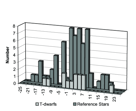
Figure 8: DCR coefficient histograms for reference stars and programme T dwarfs, in units of mas/Tan(Zenith Angle). See Section 6.1 for more details.

6.2 Photometry for L and T dwarfs

There are currently only a few large and systematic photometric databases for late M, L and T dwarfs extant. The first is the photometry from the 2MASS database Cutri et al. 2001, which has the advantage of being a well established photometric system which covers the whole sky, and includes all of our T dwarf targets, and almost of all of the other known L and T dwarfs (Burgasser, 2002a). Unfortunately, the photometry for these objects in the J and K_s 2MASS bands is often near the 2MASS photometric limits, so typical uncertainties of $\pm$0.1 mag. or greater are not uncommon. Moreover, because 2MASS does not include an optical passband, colour information has to rely on the J–K colour, which is typically small compared to the photometric precision, as well as giving only a small wavelength “lever arm” on the spectral evolution of L and T dwarfs.

We make use of absolute M_J and M_Ks values on the 2MASS system compiled by Burgasser (2002a) which is based on the parallaxes presented in Dahn et al. (2002). Dahn et al. (2002) also present optical photometry in the $I_{C}$ passband, and J,H,K photometry in a photometric system approximating that of the CIT system of Elias et al. (1982), as well as data form other work transformed onto this system.

A second extensive database is that compiled by Leggett et al. (2002). This includes Z band photometry (on a UKIRT defined photometric system) as well as J,H,K photometry transformed by the authors onto the MKO photometric system (see Leggett et al. 2002, Section 3 for details). Because these data were acquired with a 4m telescope, their photometric precision is much higher than that for 2MASS. Great care should be taken in inter-comparing these two sets of photometry – the systematic differences between the two photometric systems are very significant. This is particularly true of the Z photometric system of Leggett et al. (2002), which is based on a relatively narrow interference filter (0.851-1.056 $\mu$m) used with a HgCdTe infrared array, leading to effective wavelengths for L and T dwarfs of $\approx$1.0 $\mu$m, unlike the more common optical Z-type observations which are based on long-pass filters ($\gtrsim$0.85 $\mu$m) and the declining sensitivity of CCDs at $>$1 $\mu$m, leading to effective wavelengths $\approx$0.9 $\mu$m. . UKIRT Z photometry should not be assumed to be directly comparable with optically based Z photometry. In the discussion that follows, therefore, we will discuss only features in the absolute magnitudes within an individual photometric system. For this reason we do not make use of the more heterogeneous J,H,K compilation of Dahn et al. (2002).

To these data sets we add observations of the recently announced T dwarf $\epsilon$ Ind B Scholz et al. (2003), which has a mean I=16.7$\pm$0.1 and 2MASS photometry of J=11.91$\pm$0.04 and Ks=11.21$\pm$0.04 (Burgasser, priv.comm.).

6.3 Photometric corrections for known binaries

Figure 9: Plot of I_C–J against J–Ks for L and T dwarfs from Burgasser (2002a) and Dahn et al. (2002). The data breaks into two clear sequences for the L and T dwarfs. The solid lines are least-squares linear fits to the data as follows: for L dwarfs J–Ks = 0.707(I_C–J) - 1.003 for 3.2$<$I_C–J$<$4.4 ($\sigma=0.14$); for T dwarfs J–Ks = 7.598 - 1.371(I_C–J) for 4.4$<$I_C–J$<$6.0 ($\sigma=0.25$).

Table 3: L and T dwarf binary magnitudes

System	Comp.	$\Delta$IC	$\Delta$Ja	$\Delta$Ka	Sp.T.	Notes
2MASS J0746425+200032AB (catalog )	A	0.50	0.54	0.59	L0.5	$\Delta$IC,$\Delta$J R01. $\Delta$K Fig.9
	B	1.12	1.01	0.95	L0.5	$\Delta$IC,$\Delta$J R01. $\Delta$K Fig.9
2MASS J1146345+223053AB (catalog )	A	0.61	0.64	0.67	L3	$\Delta$IC,$\Delta$J R01. $\Delta$K Fig.9
	B	0.92	0.87	0.84	L3	$\Delta$IC,$\Delta$J R01. $\Delta$K Fig.9
2MASSs J0850359+105716AB (catalog )	A	0.29	0.55	0.26	L6	$\Delta$IC,$\Delta$J R01. $\Delta$K Fig.9
	B	1.63	0.99	1.67	T2:	$\Delta$IC R01. $\Delta$J Fig.11. $\Delta$K Fig.9
DENIS-P J0205290-115925AB (catalog )	A	0.75	0.75	0.75	L7	Assumed equal mass binary K99,L01
	B	0.75	0.75	0.75	L7	Assumed equal mass binary K99,L01
DENIS-P J1228138-154711AB (catalog )	A	0.54	0.66	0.75	L5	$\Delta$J M99, $\Delta$K K99, $\Delta$IC Fig.9
	B	1.02	0.86	0.75	L5	$\Delta$J M99, $\Delta$K K99, $\Delta$IC Fig.9
2MASS J12255432-2739466AB (catalog )	A	0.24	0.28	0.16	T6	$\Delta$IC,$\Delta$J B03, $\Delta$K Fig.9
	B	1.76	1.63	2.15	T8	$\Delta$IC,$\Delta$J B03, $\Delta$K Fig.9
2MASS J15344984-2952274AB (catalog )	A	0.53	0.75	0.75	T5.5	$\Delta$IC,$\Delta$J B03, $\Delta$K assumed 0.75
	B	1.03	0.75	0.75	T5.5	$\Delta$IC B03, $\Delta$J,$\Delta$K assumed 0.75

Several of the systems published in the photometric compilations listed above are known to be binaries, having been resolved either from the ground (Koerner et al., 1999; Leggett et al., 2001), or using HST (Martıǹ, Brander & Basri, 1999; Reid et al., 2001; Burgasser et al., 2003a). Unfortunately, not all these systems have measured magnitude differences in all the passbands of interest, so we are forced to estimate magnitudes for the A and B components of these systems based on available colour-colour relationship data. In some cases (especially 2M0850B) these extrapolations are large, and the decomposed magnitudes should be treated as indicative only. Table 3 shows the magnitude differences between each component and the total magnitude of each system, along with estimated spectral types from Burgasser et al. (2003a). Because of the similarity between the effective wavelengths of the HgCdTe-based Z and J bands, we assume that the magnitude differences in Z are the same as those derived at J. We do not differentiate here between UKIRT and 2MASS J and K bands.

2M0746AB, 2M1146AB & 2M0850AB were observed by Reid et al. (2001) in the HST F814W filter from which magnitude differences for the components were derived in the I_C passbands. Infrared J-band magnitude differences were then estimated using the L dwarf sequence of the M_I versus I_C–J colour-magnitude diagram (which has a roughly constant slope). With the exception of 2M0850B, this procedure will be adequate for all the L dwarfs, and those values are shown in Table 3. 2M0850B is an exception because its absolute magnitude at I_C is so faint that it must be an early- to mid-T dwarf, rather than an L dwarf. And, as we show in Section 6.5, the colour-magnitude diagram is not even remotely linear across the L-T dwarf transition. For 2M0850B, therefore, we have used the M_I for the AB system of Dahn et al. (2002), and the magnitude differences of Reid et al. (2001) to derive for the B component M_I = 20.02$\pm$0.23. The colour-magnitude diagrams in Section 6.5 then imply I_C–J $\approx$ 5.1$\pm$0.2, from which we derive the B component J magnitude difference shown in the Table.

To derive K-band magnitudes for the components of these systems, we have plotted J–Ks versus I_C–J for all the L and T dwarfs in Burgasser (2002a) and Dahn et al. (2002) in Figure 9. The data reveal two separate sequences – the L dwarfs in which J–Ks becomes redder along with I_C–J, and the T dwarfs in which the reverse holds. The two lines on the plot are linear fits to these two regimes (arbitrarily divided at I_C–J=4.4). From these relations we predict J–Ks colours for L and T dwarfs from their I–J colours, and so derive the magnitude differences for each component in Table 3.

D0205AB & D1228AB were both observed by Koerner et al. (1999) in the K band at Keck, and D0205AB was independently observed at UKIRT by Leggett et al. (2001). D1228 was also observed in the J band with HST by Martıǹ, Brander & Basri (1999). D0205 was found to be a pair of objects with equal brightness at K, and in the absence of any other information we assume it to be an equal mass binary. D1228 is a nearly equal mass binary – from the marginal J–K colour difference between the two components we can extrapolate to a magnitude difference between the components at I of 0.48.

2M1225AB, 2M1534AB have been observed by Burgasser et al. (2003a) with HST in the F814W and F1042M filters (the latter enabling the derivation of approximate J magnitude differences for the systems). Once again we use the I–J colours of these objects to extrapolate to K magnitude differences for 2M1225AB’s components. For 2M1534AB the magnitude differences estimated at F1042 are only marginally different from zero, so we assume equal brightnesses in this system at J and K.

6.4 Spectral-Type-Magnitude relations for L and T dwarfs

Table 4: T dwarf Photometry & Absolute Magnitudes for NTT Parallax Sample

Object	T	2MASS		MKO			2MASS		MKO
		J	Ks	J	K	Z-J	MJ	MKs	MZ	MJ	MK
SD1021	T3	16.26$\pm$0.10	15.10$\pm$0.18	15.88	15.26	1.78	13.94$\pm$0.29	12.78$\pm$0.33	15.34$\pm$0.27	13.56$\pm$0.27	12.94$\pm$0.27
2M1047	T6.5	15.82$\pm$0.06	16.30$\pm$0.30:	15.46	16.20	1.93	16.05$\pm$0.14	16.52$\pm$0.33	17.61$\pm$0.13	15.68$\pm$0.13	16.42$\pm$0.13
2M1217	T7.5	15.85$\pm$0.07	15.90$\pm$0.30:	15.56	15.92	2.00	15.64$\pm$0.09	15.69$\pm$0.30	17.35$\pm$0.06	15.35$\pm$0.06	15.71$\pm$0.06
2M1225	T6	15.22$\pm$0.05	15.06$\pm$0.15	14.88	15.28	1.89	14.60$\pm$0.09	14.44$\pm$0.17	16.15$\pm$0.08	14.26$\pm$0.08	14.66$\pm$0.08
SD1254	T2	14.88$\pm$0.04	13.83$\pm$0.06	14.66	13.84	1.74	14.20$\pm$0.07	13.15$\pm$0.08	15.72$\pm$0.06	13.98$\pm$0.06	13.16$\pm$0.06
2M1346	T6	15.86$\pm$0.08	15.80$\pm$0.30:	15.49	15.73	2.24	15.03$\pm$0.11	14.97$\pm$0.31	16.90$\pm$0.08	14.66$\pm$0.09	14.90$\pm$0.08
2M1534	T5.5	14.90$\pm$0.04	14.86$\pm$0.11	14.60	14.91		14.24$\pm$0.05	14.19$\pm$0.12		13.94$\pm$0.05	14.25$\pm$0.05
2M1546	T5.5	15.60$\pm$0.05	15.42$\pm$0.17				15.32$\pm$0.07	15.14$\pm$0.18
SD1624	T6	15.49$\pm$0.06	15.40$\pm$0.30:	15.20	15.61	2.12	15.28$\pm$0.07	15.19$\pm$0.30	17.11$\pm$0.04	14.99$\pm$0.04	15.40$\pm$0.06

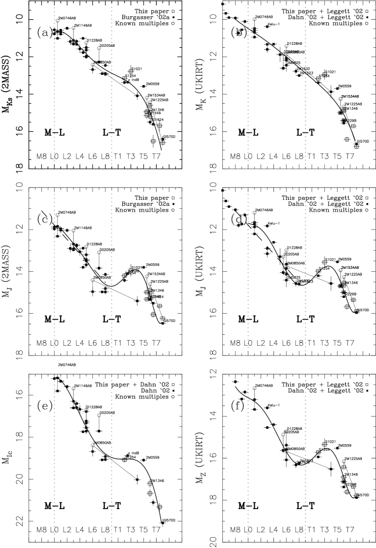
Figure 10: Absolute magnitudes in a variety of bandpasses, as a function of L and T spectral types on the Kirkpatrick et al. and Burgasser et al. systems. Panels (a) and (c) show absolute M_J and M_Ks from 2MASS photometry in Burgasser (2002a); Scholz et al. (2003) and this paper. Panels (b),(d) and (f) show absolute M_J, M_K and M_Z on the Leggett et al. (2002) UKIRT system. Panel (e) shows M_Ic from photometry in Dahn et al. (2002). All parallaxes are from either this work (open squares) or Dahn et al. (2002) & Scholz et al. (2003) (filled squares). The dotted line in panels (c) and (d) is the spectral-type-magnitude relation of Dahn et al. (2002). Known unresolved binaries are encircled, and decomposed into their resolved components as described in Section 6.3. The solid heavy lines are seventh-order polynomial weighted fits to the data (see Section 6.8 for coefficients). The decomposed JK magnitudes and spectral type of 2M0850B are much more uncertain than the formal uncertainties plotted would indicate, and should be treated as indicative only.

Table 4 lists Burgasser (2002a), Dahn et al. (2002) and Leggett et al. (2002) photometry for our NTT parallax sample, along with the resulting absolute magnitudes in these systems. Also listed are spectral types on the scheme of Burgasser et al. (2002b).

Figure 10 shows plots of spectral type against M_Z, M_I, M_J and M_Ks/M_K. Also shown are absolute magnitudes for late M and L dwarfs using parallaxes and 2MASS photometry from Dahn et al. (2002) for the 2MASS panels, and parallaxes from Dahn et al. (2002) and UKIRT photometry from Leggett et al. (2002) for the UKIRT panels. The spectral types are on the system of Kirkpatrick et al. (1999) for the M and L dwarfs, and Burgasser et al. (2002b) for the T dwarfs. Known multiple systems are noted with circles, and decomposed into their component magnitudes as discussed above.

The two K-band plots (Fig. 10a and 10b) indicate that in both systems, the L-T transition is marked by a steepening of the spectral-type-magnitude relation. In general, however, the relationship between absolute magnitude at K and spectral type is well behaved for the purpose of estimating absolute magnitudes from spectral types. This is certainly not true in the 2MASS and UKIRT J passbands (Fig. 10c and 10d). Indeed, both sets of data indicate a strong inflection (a “hump”) in the relationship between absolute magnitude and spectral type for early T dwarfs – as a class, the T0-T4 brown dwarfs have absolute magnitudes brighter than the latest L dwarfs by a magnitude or more. Put another way, a simple extrapolation of the spectral-type-magnitude relationship for L dwarfs (eg. that from Dahn et al. (2002) shown in the figure) underestimates the absolute magnitude of the early- to mid-T dwarfs by up to two magnitudes. This “early T hump” has been noted previously (Dahn et al., 2002), though on the basis on fewer T dwarf parallaxes. It has been suggested (Burgasser, 2002a) that binarity could be the cause for early T dwarfs being more luminous than the late L dwarfs. While it is certainly true that the L and T dwarfs which have been resolved as binaries are displaced to apparently high absolute magnitudes when plotted as unresolved objects, the addition of new parallaxes would seem to indicate the over-luminosity of early T dwarfs is a general property, rather than being due to the selection of objects which happen to be binaries. Moreover, the magnitude or more of over-luminosity is too large an effect to be due equal-mass binarity which can produce a brightening of only 0.75 mag. A similar (though possibly less pronounced) inflection is seen in the M_Z relation (Fig. 10f), while the M_I relation (Fig. 10e) would appear to be almost as monotonic as that at K, though with a more pronounced inflection at the L-T boundary. Having said this, however, 2M0559 continues to appear to be over-luminous compared to the other early- to mid-T dwarfs in the figure. Burgasser et al. (2003a) failed to resolve a binary companion in this system with HST, implying that if it is a binary it must have a separation of less than 0.5 a.u. We also note that it has been suggested (Tsuji & Nakajima, 2003) that the selection of preferentially young objects could produce the “early T hump” – we discuss this further in Section 6.6.2.

There are good physical reasons for expecting a monotonic relationship between effective temperature (T_eff) and luminosity (L) in these objects, since these quantities are directly determined by interior (rather than photospheric) properties. However, it must be remembered that as proxies for T_eff and luminosity, absolute magnitude in a given passband and spectral type are far from perfect. Spectral typing is in essence an arbitrary allocation of a quantity to an object based on what its spectra look like – there is no guarantee that the relationship between spectral type and T_eff (even if monotonic) should not have significant changes in slope. Similarly, the relationship between absolute magnitude in a given passband and luminosity is even more problematic. From the spectra of objects ranging from L to T spectral types, and indeed from their J–K colours (Dahn et al., 2002), we know that significant changes take place in their photospheres. There is significant redistribution of flux in the spectra of brown dwarfs across the L-T transition. We should not be surprised if this results in the relationship between luminosity absolute magnitude in a given passband not only containing changes in slope, but not even being monotonic.

Given our current parallax database, spectral type is a very poor proxy for absolute magnitude in the Z and J bands from mid-L to mid-T spectral types. The sequences in Fig.10 will need to be filled in by many more L and T dwarfs before precise absolute magnitudes can be estimated from spectral types with confidence.

6.5 Colour Magnitude Diagrams for L and T dwarfs

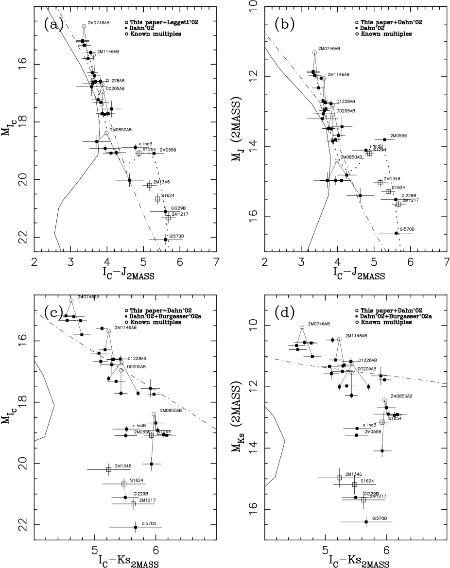
Figure 11: Colour magnitude diagrams based on I_C and 2MASS J,Ks photometry (Dahn et al., 2002; Burgasser, 2002a)), and the parallaxes of this paper and Dahn et al. (2002); Scholz et al. (2003). Symbols are as for Fig. 10. The solid lines are 1 Gyr isochrones from the COND models of Baraffe et al. (2003), and the dot-dashed lines are the 1 Gyr isochrones from the DUSTY models of Chabrier et al. (2000); Allard et al. (2001). Both sets of models are have been kindly recalculated in the 2MASS & I_C filter systems by I.Baraffe. The dotted lines in panels a and b are high-order polynomial fits to the data – see Section 6.8. The decomposed J and K magnitudes of 2M0850B are much more uncertain than the formal uncertainties plotted would indicate, and should be treated as indicative only.

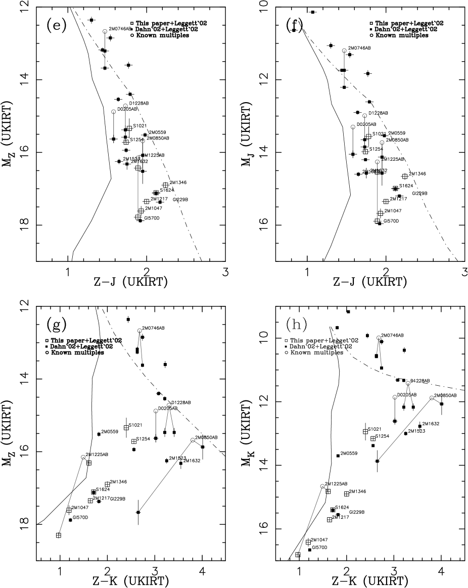
Figure 11(cont.): Colour magnitude diagrams based on UKIRT Z,J,K photometry (Leggett et al., 2002)), and the parallaxes of this paper and Dahn et al. (2002); Scholz et al. (2003). Symbols are as for Fig. 10. The solid lines are 1 Gyr isochrones from the COND models of Baraffe et al. (2003), and the dot-dashed lines are the 1 Gyr isochrones from the DUSTY models of Chabrier et al. (2000); Allard et al. (2001). Both sets of models are have been kindly recalculated in the UKIRT filter system by I.Baraffe. The decomposed J and K magnitudes of 2M0850B are much more uncertain than the formal uncertainties plotted would indicate, and should be treated as indicative only.

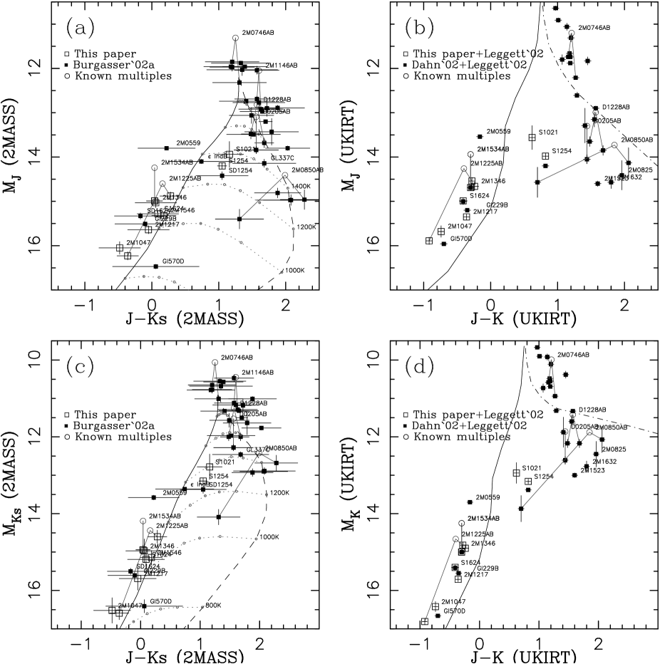
Figure 13: Colour magnitude diagrams using J-K colours on the 2MASS (panels a and c Dahn et al. 2002; Burgasser 2002a) and UKIRT (panels b and d, Leggett et al. 2002 systems. Parallaxes from this paper and Dahn et al. (2002); Scholz et al. (2003). The isochrones shown in panels (b) and (d) are 1 Gyr DUSTY (dot-dashed line) and COND (solid line) models of Baraffe et al. (2003); Chabrier et al. (2000); Allard et al. (2001). The isochrones in panels (a) and (c) are the CLEAR (solid line) and CLOUDY (dashed line) models presented in Burgasser et al. (2002c). Joining these are dotted lines for the “Cloud Clearing” interpolations between these models with small circles highlighting the 20%, 40%, 60% and 80% interpolation levels at effective temperatures of 800, 1000, 1200, 1400, 1600 & 1800K. The decomposed J and K magnitudes of 2M0850B are much more uncertain than the formal uncertainties plotted would indicate, and should be treated as indicative only.

Using the same photometry, we can construct a variety of colour-magnitude diagrams. Figure 11 shows such diagrams based around Cousins I_c, UKIRT Z and both UKIRT and 2MASS J,K photometry, while Figure 13 shows similar diagrams for UKIRT and 2MASS J–K colours. The most noticeable feature of these diagrams is how few are actually useful as traditional colour-magnitude diagrams – almost none show the simple monotonic relationships between absolute magnitude and colour which hold for stars and brown dwarfs down to the early L dwarfs.

Fig 11c,d show that I–K colours jumps to the blue by I–K$\approx$0.5 mag as the L-T transition is crossed at M_I$\approx$19, M_K$\approx$ 13, but then tends redward again for later and later T dwarfs. However, Gl 570D, one of the latest and faintest T dwarfs currently known, never becomes as red as the latest L dwarfs. This blueward jump is particularly pronounced at M_I where the absolute magnitudes of L8 and early T dwarfs are indistinguishable. As a result I–K should be considered a poor indicator for determining the absolute magnitude or effective temperature of late L to late T dwarfs. In particular, and luminosity function based on I–K$\gtrsim$5 will be subject to serious biases which will introduce completely spurious structure into the luminosity function.

Fig 11a,b shows that I–J colour-magnitude diagrams can be considered the “best of a bad bunch” when it comes to the traditional use of colour-magnitude diagrams (i.e. estimating absolute magnitudes from photometric colours), since the cooling curves of brown dwarfs do not reverse in I–J as they do for every other panel of Figs 11 and 13. Even so, between I–J=4 and I–J=5 they show the same pronounced “S-curve” seen in the spectral type data of Fig. 10, with early T dwarfs being up to a magnitude brighter in M_J than late L dwarfs. And, once again we see that 2M0559 appears anomalously bright, suggestion binarity in spite of Burgasser et al. (2003a)’s failure to resolve it with HST..

The Z–J colour-magnitude diagrams (Fig.11e,f) reveal a very steep colour-magnitude relation, with scatter which is significantly larger than the photometric errors. The slope of the colour-magnitude relation is so steep that no meaningful estimate of M_Z or M_J can be derived from a Z–J colour. This is not surprising, given the very close effective wavelengths of HgCdTe-based Z and J photometry. There is some evidence for trend at the bottom of this colour-magnitude diagram that at M${}_{Z}\gtrsim 16.5$ and M${}_{Ks}\gtrsim 14.5$, Z–J colours becomes bluer for fainter and later-type objects.

Colour magnitude diagrams involving Z–K (Figs 11g-h) and J–K (Figs 13a-d) show an especially pronounced reversal of the brown dwarf cooling curves beyond M${}_{K}\approx 12.5$, M${}_{J}\approx 14$ and M${}_{Z}\approx 16$. This has been noted in J–K colour-magnitude diagrams by several authors (e.g. Burgasser et al. 2002c). Major changes take place in photospheres below the L-T transition, with the result that T dwarfs swap from very red, to very blue, J–K colours. It is interesting that the Z–K diagrams show almost identical behavior, with Z–K colours for the very faintest T dwarfs becoming as blue as Z-K$\approx$-1. This compares with colours based on the SDSS $z^{\prime}$ filter (see eg.Dahn et al. 2002 Fig. 3) which continue to become redder for the latest T dwarfs. This once again clearly demonstrates the considerable difference between CCD-based $z^{\prime}$, and the HgCdTe-based Z.

There is a clear warning to astronomers implicit in these diagrams – conclusions reached about luminosity- and mass-functions based on luminosity and/or colours for the L-T effective temperature range are fraught with difficulty. In particular, luminosity functions determined from the colours of objects in field samples will produce completely spurious features in the derived luminosity- and mass-functions, unless the various “bumps and wiggles” in these diagrams are adequately and correctly modeled. (See for example Reid & Gizis (1997)’s demonstration of the formation of a “false” peak in M dwarf luminosity function based on the traditional – and inadequate – parametrization of the M dwarf colour-magnitude relation). Similarly, determining bolometric luminosity functions from apparent magnitudes in cluster-based samples is problematic, as we can expect similar “bumps and wiggles” to be present in the bolometric correction relations for the L and T dwarfs.

Features like these can introduce significant systematic biases into the mass functions derived from even a perfect statistical sample. Actual statistical data with all the added complexities of uncertain age and binarity distributions add yet more complications. Monte Carlo simulations are essential to the interpretation of any luminosity- or mass-function in the L-T effective temperature range. it is important to carefully “reverse” model such functions from sets of mass-function models, through a variety of possible colour-magnitude and bolometric-correction relations (as allowed by the extant data), to sample observational data. Then such artificial data can then be meaningfully compared to statistical samples in the observational plane. Mass- or luminosity functions which do not include such extensive reverse modeling should be treated with the utmost suspicion.

6.6 Theoretical Models for L and T dwarfs

Ultra-cool dwarfs are notoriously difficult to model – the components which need to be included in models for L and T dwarfs include (Allard et al., 1997): the effects of tens of millions of molecular transitions in species including H₂O, CH₄, TiO, VO, CrH, FeH, and a host of others; complex treatments of the line wings of enormously H₂ and He pressure-broadened neutral alkali lines like K and Na, Rb and Cs; collision-induced molecular H₂ opacity; both the chemistry and opacity involved in the condensation, settling, revapourisation and diffusion of a variety of condensates including liquid Fe, solid VO, and a range of aluminium, calcium, magnesium and titanium bearing refractories; and finally (and least readily modeled of all) the effects of rotation-induced weather on the cloud decks which condensates will form.

Significant progress has been made in recent years on the detailed solution of photospheric models using very large line lists (see Allard et al. (1997) for a review). Probably the largest outstanding problem for modelers of L and T dwarfs is dealing with condensation. Three approximations to this complex situation have currently been implemented. “Dusty” models (eg. the DUSTY model of Allard et al. 2001) assume condensates remain well suspended and in chemical equilibrium where they form in the photosphere. In general such models have been shown to work reasonably well for L dwarfs, suggesting that their cloud layers lie within their photospheres. “Condensation” models (eg. the COND models of Baraffe et al. 2003, and the CLEAR models of Burrows et al. 1997) neglect dust opacities, to simulate the removal of all condensates from the photosphere as they form (most likely through gravitational settling). The “CLOUDY” models of Ackerman & Marley (2001) and Marley et al. (2002) incorporate a model for condensate cloud formation, based on an assumed sedimentation efficiency parameter $f_{rain}$.

6.6.1 Colour-magnitude diagrams in J–K and Z–K

Figures 11 and 13 have over-plotted on them a variety of these models, including the DUSTY (Chabrier et al., 2000; Allard et al., 2001) and COND models (Baraffe et al., 2003) for an age of 1 Gyr, and the CLEAR and CLOUDY models as presented in Burgasser et al. (2002c) for $f_{rain}=3$ (determined as the best fit for this model in Jupiter’s ammonia cloud deck Marley et al. 2002). As previous studies have shown, DUSTY models reproduce the general features (if not the precise colours) of the cooling curves for L dwarfs, but then proceed to much redder colours than are observed beyond L8. This has been interpreted as indicating that condensates are present in the photosphere of L dwarfs. The COND and CLEAR models reproduce the general features of the cooling curves for late T dwarfs, indicating that at these effective temperatures condensate opacities do not contribute to the radiative transfer, which suggests that the condensate layers have dropped below the photosphere. DUSTY and CLEAR/COND models, therefore, describe the “boundary conditions” to the condensate opacity problem, and are appropriate for the L and late T types respectively. But what about the intermediate case which must be appropriate to early T dwarfs? This is exactly the situation with the sedimentation models of Marley et al. (2002) should be able to address.

Burgasser et al. (2002c) compared their CLOUDY models for $f_{rain}=3$ with a 2MASS M_J:J-K colour-magnitude diagram (as we do in Fig. 13). As for the DUSTY models, the CLOUDY models predict the general behaviour of L dwarfs, and then veer towards bluer J–K colours at late T dwarf temperatures. However, this transition does not match the observed sequence, which transitions nearly horizontally between the L dwarf/DUSTY/CLOUDY sequence and late-T dwarf/CLEAR/COND model at M_J$\approx$14, M_Ks$\approx$13. (We note that though the equivalent models are not available in the UKIRT Z,J,K bandpasses, very similar behaviour is seen in Fig. 11, with a clear transition between the L dwarf and late T dwarf sequences.) Burgasser et al. (2002c) suggested that a possible resolution for this discrepancy could be the appearance of uneven cloud cover on the surface of early T dwarfs. This would allow the emergent spectrum to appear as a “mixture” of the CLEAR/COND and CLOUDY spectra. They modeled this by interpolating between their CLEAR and CLOUDY models at effective temperatures of 800 K, 1000 K, 1200 K, 1400 K, 1600 and 1800 K with varying fractions of the two models (ie. 20%,40%,60 & 80%). The tracks for these “mixture” models are shown in Fig. 13 as dotted lines, and suggest that there is a transition sequence between L and T dwarfs at T_eff $\approx$ 1300K. SDSS1021, SDSS1254, 2M1225, $\epsilon$ Ind B and possibly 2M0850B (though with some uncertainty because of the poor quality of its decomposed secondary flux) fill out this transition region. The status of 2M0559 is unclear. If it is a single object, then it probably represents the ‘top’ of the late T dwarf cooling sequence, which is $>$1 mag. brighter in M_J than the bottom of the L dwarf sequence. If however, it is a binary, then the prototype for the ‘top’ of the late T dwarf cooling sequence is probably more like the object 2M1225A or 2M1346 at a spectral type of T5.5-T6. The “transition temperature” indicated by the additional T dwarfs in this work is slightly warmer ($\approx$1300K) than that found by Burgasser et al. (2002c).

An alternative dust model to the sedimentation models of Marley et al. has been developed by Tsuji & Nakajima (2003). These “Unified Cloudy Models” (UCM) are built around a single thin dust layer in which particles of size greater than a critical radius are removed from the photosphere by sedimentation. This critical radius is parametrized by a critical temperature $T_{cr}$ below which dust particles sediment, which is determined by comparing model results to colour-magnitude diagrams. This single model has the advantage of predicting the gross behaviour of brown dwarfs as they transition from L to T spectral types, with a single model. Unfortunately, (Tsuji & Nakajima, 2003, Fig.2) the detailed behaviour of the models does not match observations. In particular, UCM cannot make L dwarf as red or faint in M_J:J–K as they actually appear. Nor does it predict the observed brightening of the “early T dwarf hump” other than as an age-selection effect, which we conclude below, is not the case.

It should be noted, however, that the interpretation of Marley et al. models and data in Fig. 13 in terms of cloud openings (i.e. as providing evidence for the existence of weather in early T dwarfs) is quite dependent on the details present in the Marley et al. (2002) models. An independent test of this conclusion is clearly desirable. Fortunately, Fig. 13 indicates that J and K band time-series photometry can provide that test. The location of a given object on the “transition sequence” will depend critically on its fractional cloud cover. Because this could be expected to change as each brown dwarf rotates, a statistical study of the J-band variability from late L dwarfs to late T dwarfs should find stronger variability in early T dwarfs, than in late L dwarfs or late T dwarfs.

Finally, we note that although the COND models do not do a very good job of predicting the absolute colours of late T dwarfs in Z–J and Z–K (Fig. 11e-h), they do suggest a trend for late T dwarfs to become bluer in both Z–J and Z–K as they get colder and fainter than M_J$\approx$14.5 and M_K$\approx$14.75. Moreover, the available data suggest this trend is real, though the absolute colours of T dwarfs at these magnitudes are somewhat redder than the models would predict.

6.6.2 The “Early T Hump”

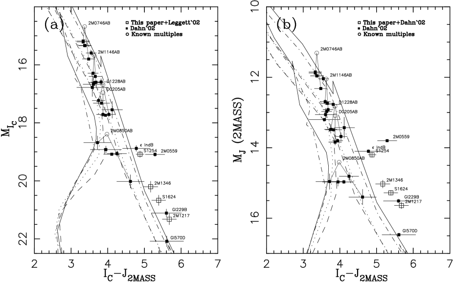
Figure 14: Colour magnitude diagrams based on I_C and 2MASS J photometry (Dahn et al., 2002; Burgasser, 2002a)), and the parallaxes of this paper and Dahn et al. (2002); Scholz et al. (2003). DUSTY (Chabrier et al., 2000; Allard et al., 2001) (rightmost lines) and COND Baraffe et al. (2003) (leftmost lines) are shown as in Fig. 11, but now for a range of ages: 50 Myr (solid), 100 Myr (dot-dashed), 1 Gyr (dotted), 5 Gyr (dashed).

The M_J:I_C–J colour-magnitude diagrams shown in Fig. 11a-b indicate a remarkable brightening at M_J for the observed early T dwarfs. Unfortunately, neither the COND nor the DUSTY models indicate why this should be so. The DUSTY models predict an extension of the L dwarf sequence, which we have good reason to believe is not correct, based on the analysis of colour-magnitude diagrams in J–K above. Unfortunately, the COND models also fail to look even remotely like the available data for T dwarfs in Fig. 11a-d. Shortcomings in these models at short wavelengths have been noted by Baraffe et al. (2003), which are thought to be due to an inadequate treatment of the extremely broad wings of the K and Na lines at these wavelengths.

One possible interpretation of the “early T hump” in Fig. 11a-b, is that it could be a gravity effect (Tsuji & Nakajima, 2003). Very young brown dwarfs will have isochrones slightly offset to brighter magnitudes than older brown dwarfs, because of their lower gravities. This effect is particularly pronounced in photospheres in which dust is an important opacity source. It is possible then that the “early T hump” could be produced by the preferential selection of young, bright brown dwarfs.

Fig. 14 plots the same data as that shown in Fig. 11a-b, but now we plot four isochrones spanning 50 Myr-5 Gyr to examine the effects of age. The figure shows that, as expected, the DUSTY models (most appropriate for L dwarfs) show significant offsets in their isochrones of a magnitude or more between 50 Myr and 5 Gyr. These offsets are not as marked for the COND models. Unfortunately, interpreting the “early T hump” as an age effect is severely complicated by the fact that it occurs at exactly the point where there is good evidence to believe neither the DUSTY or COND models are working.

For the L dwarfs and late T dwarfs, the spread in the colour-magnitude diagram is not pronounced, (particularly when known binaries are decomposed), suggestive of the small 100 Myr – 1 Gyr age spread seen in other studies of L and T dwarfs (Dahn et al., 2002; Scholz et al., 2003). It is certainly nowhere near as pronounced as would be necessary to produce the age spread required to account for the more than 1 magnitude brightening of the“early T hump” all by itself. Moreover, there is a definite spectral type trend along the track represented by the “early T hump”, as seen in the spectral-type-magnitude diagrams of Fig. 10 – from the late L dwarfs, through $\epsilon$ Ind B, SD1254, SD1021 to 2M0559. This same trend is seen in the colour-magnitude diagrams. We interpret this as indicating that the “early T hump” truly is a feature in the cooling curve of brown dwarfs, rather than an artifact of youth and selection.

6.7 The Onset of CH₄ absorption in Clusters

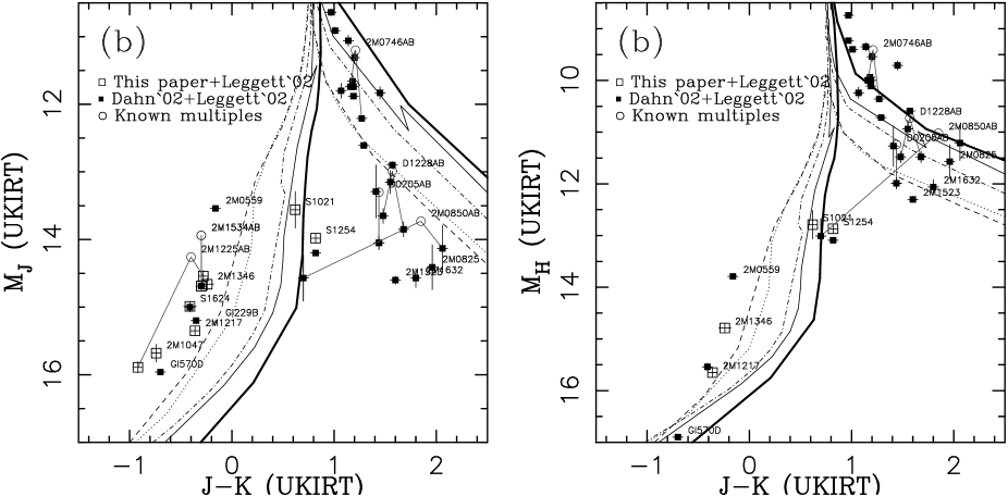
Figure 15: Colour magnitude diagrams in UKIRT M_J and M_H vs J–K. DUSTY (Chabrier et al., 2000; Allard et al., 2001) (rightmost lines) and COND Baraffe et al. (2003) (leftmost lines) are shown as in Fig. 11, but now for a range of ages: 10 Myr,(heavy solid) 50 Myr (solid), 100 Myr (dot-dashed), 1 Gyr (dotted), 5 Gyr (dashed). The decomposed J and H magnitudes of 2M0850B are much more uncertain than the formal uncertainties plotted would indicate, and should be treated as indicative only.

Methane filters centered on the strong CH₄ absorption bands in the H-band have been acquired by a number of observatories for use in their infrared cameras. Given we have now measured just where, in absolute magnitude, the T dwarf class occurs, the question arises, “At what magnitudes will CH₄ absorption in young star clusters set in?” Fig. 15 shows UKIRT M_J and M_H:J–K colour-magnitude diagrams, along with the DUSTY and COND models at ages from 10 Myr to 5 Gyr. Based on these diagrams, we can conclude that for field T dwarfs, as discovered by the 2MASS and SDSS surveys, CH$4$ absorption (corresponding to spectral classes around T2 and later) sets in at at M_H$\approx$13, and somewhat more confusingly at M_J$\sim$14 – though because of the brightening of “early T hump” at J non-CH₄-absorbing L dwarfs will actually be fainter than the earliest CH₄ absorbing T dwarfs.

Because the turn on of CH₄ absorption is primarily an effect driven by effective temperature, to first order it will occur at the same absolute magnitude in young clusters as it does in the field. Looked at in slightly more detail, however, we can see that for a given colour in Fig. 15, there is a small offset to brighter magnitudes for younger objects – in the DUSTY atmosphere case a 10 Myr dwarf at the end of the L8 sequence will be $\approx$1.0 mag. brighter than a 1 Gyr dwarf of the same colour and effective temperature, and 1.3 mag brighter than a 5 Gyr dwarf. In the COND case the equivalent differences are 1.3 and 1.7 magnitudes. The likely ages for our field T dwarfs will be somewhere in the range 100 Myr-1 Gyr (Dahn et al., 2002; Scholz et al., 2003). This would suggest that in clusters like IC 2391 or IC 2602 of age 10-20 Myr at d$\approx$150 pc the absolute magnitude for CH₄ onset will be M_H$\sim$12-12.5, or equivalently H$\sim$18-18.5. For older clusters like the Pleiades (100 Myr, d$\sim$125 pc) these numbers are more like M_H$\sim$12.5-13 or H$\sim$18-18.5.Both of these are eminently reachable magnitude limits with wide-field cameras on 4m-class telescopes, suggesting that CH₄ imaging may be a powerful tool for easily conducting an unbiased census of T dwarfs in large open clusters. Similarly for more compact, but distant clusters, like Trapezium ($\sim$25 Myr, 450 pc) observations at H$\sim$20-20.5 are tractable over the fields-of-view required on 8m-class telescopes.

Fig. 15 also has implications for the interpretation of potential cluster membership. For example, Zapatero Osorio et al. (2002) have found a T6 dwarf in the direction of the $\sigma$ Orionis cluster. Fig. 15 suggests that a field brown dwarf of this spectral type will have M_H=15.0$\pm$0.5. For the much younger age of $\sigma$ Orionis (1-8 Myr Zapatero Osorio et al. 2002) this will be more like M_H=14.0$\pm$0.5, which would imply a distance to the $\sigma$ Ori J053810.1-023626 T6 dwarf of 192$\pm$50 pc – more consistent with being a foreground object than a member of the cluster at d=352 pc (Perryman et al., 1997).

6.8 Colour-Magnitude & Spectral-Type-Magnitude relations for L and T dwarfs

Figures 10 and 11 have over-plotted on some of their panels high-order polynomial fits to the weighted (and binary decomposed) data. As inspection of the figures shows, these fits are not always particularly successful at modeling the extremely complex behaviour of these cooling curves in the observed passbands. Nonetheless, in the absence of working atmospheric models the fits may be a useful tool, so long as their weaknesses are acknowledged. We therefore provide the coefficients for these fits, and the root-mean-square scatter about the fits in Table 5.

Table 5: Polynomial coefficients for plotted fits

$P(x)$	$x$	RMS	$c_{0}$	$c_{1}$	$c_{2}$	$c_{3}$	$c_{4}$	$c_{5}$	$c_{6}$	$c_{7}$
MKs (2M)	SpT	0.38	6.27861e$+$1	-1.47407e$+$1	1.54509e$+$0	-7.42418e$-$2	1.63124e$-$3	-1.25074e$-$5	-	-
MK (U)	SpT	0.40	8.14626e$-$1	2.95440e$+$0	-3.89554e$-$1	2.68071e$-$2	-8.86885e$-$4	1.14139e$-$5	-	-
MJ (2M)	SpT	0.36	8.94012e$+$2	-3.98105e$+$2	7.57222e$+$1	-7.86911e$+$0	4.82120e$-$1	-1.73848e$-$2	3.41146e$-$4	-2.80824e$-$6
MJ (U)	SpT	0.30	5.04642e$+$1	-3.13411e$+$1	9.06701e$+$0	-1.30526e$+$0	1.03572e$-$1	-4.58399e$-$3	1.05811e$-$4	-9.91110e$-$7
MIc	SpT	0.37	7.22089e$+$1	-1.58296e$+$1	1.56038e$+$0	-6.49719e$-$2	1.04398e$-$3	-2.49821e$-$6	-	-
MZ (U)	SpT	0.29	4.99447e$+$1	-3.08010e$+$1	8.96822e$+$0	-1.29357e$+$0	1.02898e$-$1	-4.57019e$-$3	1.05950e$-$4	-9.97226e$-$7
MIc	IC–J	0.67	1.17458e$+$3	-1.22891e$+$3	5.00292e$+$2	-9.70242e$+$1	8.86072e$+$0	-2.97002e$-$1	-	-
MJ (2M)	IC–J	0.63	1.52199e$+$3	-1.69336e$+$3	7.41385e$+$2	-1.58261e$+$2	1.64657e$+$1	-6.66978e$-$1	-	-

7 Conclusion

We have shown that high precision parallaxes can be obtained with common-user near-infrared cameras using techniques very similar to those used in optical CCD astrometry. The new generation of large format infrared imagers based on HAWAII1 (1K) and HAWAII2 (2K) HgCdTe arrays, and the new generation of large format InSb arrays, offer exciting prospects for the astrometry of cool brown dwarfs in the future. Due to their infrared methane absorption bands, T dwarfs have quite similar effective wavelengths to the ensemble of background reference stars, which makes the correction of differential colour refraction effects considerably easier. The “early T hump” (i.e. the brightening at the J band of early T dwarfs relative to late L dwarfs) appears to be a feature of brown dwarf cooling curves, rather than an effect of binarity or age. And finally, these data imply that detection of T dwarfs in clusters can be made directly at tractable magnitudes in the H-band, opening the way to a new generation of cluster mass function studies based on the powerful technique of CH₄ differential imaging.

References

- Ackerman & Marley (2001) Ackerman, A.S. & Marley, M.S. 2001, ApJ, 556, 872
- Allard et al. (1997) Allard, F., Hauschildt, P.H., Alexander, D.R. & Starrfield, S.1997, ARA&A, 35, 137
- Allard et al. (2001) Allard, F., Hauschildt, P.H., Alexander, D.R.; Tamanai, A., & Schweitzer, A., 2001, ApJ, 556, 357
- Baraffe et al. (2003) Baraffe, I., Chabrier, G., Barman, T.S., Allard, F. & Hauschildt, P. 2003, A&A, submitted. astro-ph/0302293
- Burgasser et al. (1999) Burgasser, A. J., et al. 1999, ApJ, 522, L65
- Burgasser et al. (2000a) Burgasser, A. J., et al. 2000a, ApJ, 531, L57
- Burgasser et al. (2000b) Burgasser, A. J., et al. 2000b, AJ, 120, 1100
-
Burgasser (2002a)
Burgasser, A. J., 2002a, PhD Thesis, California Institute of Technology, Pasadena: California
www.astro.ucla.edu/~adam/homepage/research/tdwarf/thesis/ - Burgasser et al. (2002b) Burgasser, A. J., et al. 2002b, ApJ, 564, 421
- Burgasser et al. (2002c) Burgasser, A. J., et al. 2002c, ApJ, 571, L151
- Burgasser et al. (2003a) Burgasser, A. J., Kirkpatrick, J.D., Reid, I.N., Brown, M.E., Miskey, C.L. & Gizis, J.E., 2003a, ApJ, 586, 512
- Burrows et al. (1997) Burrows, A. et al. 1997, ApJ, 491, 856
- Chabrier et al. (2000) Chabrier, G., Baraffe, I., Allard, F. & Hauschildt, P., ApJ, 542, 464
- Close et al. (2003) Close, L.M., Siegler, N., Freed F., Biller, B. 2003, ApJ, in press. astro-ph/0301095
- Cuby et al. (2000) Cuby, J.G. et al. 2000, A&A, 349, L41
-
Cutri et al. (2001)
Cutri, R. et al. 2001, Explanatory Supplement to the 2MASS Second Incremental Data Release.
www.ipac.caltech.edu/2mass/releases/second/doc/explsup.html - Dahn et al. (2002) Dahn, C.C. et al. 2002, AJ, 124, 1170
- Elias et al. (1982) Elias, J.H., Frogel, J.A., Matthews, K. & Neugebauer, G. 1982 AJ, 87, 1029
-
Finger & Nicolini (1998)
Finger, G. & Nicolini, G. 1998, “Interquadrant Row Crosstalk”, Garching: Germany.
www.eso.org/~gfinger/hawaii_1Kx1K/crosstalk_rock/crosstalk.html - Geballe et al. (2002) Geballe, T.R. et al. 2002, ApJ, 564, 466
- Jones (2000) Jones, H.R.A. 2000, HIPPARCOS and the Luminosity Calibration of the Nearer Stars, 24th IAU General Assembly, Joint Discussion 13, Manchester, UK.
- Kirkpatrick et al. (1999) Kirkpatrick, J. D., et al. 1999, ApJ, 519, 802
- Koerner et al. (1999) Koerner, D.W., Kirkpatrick, J. D., McElwain, M.W. & Bonaventura, N.R. 1999, ApJ, 526, L25
- Leggett et al. (2000) Leggett, S. K., et al. 2000, ApJ, 536, L35
- Leggett et al. (2001) Leggett, S.K., Allard, F., Geballe, T.R., Hauschildt, P.H., Schweitzer, A. 2001, ApJ, 548, L908
- Leggett et al. (2002) Leggett, S. K., et al. 2002, ApJ, 564, 452
- Marley et al. (2002) Marley, M.S., Seager, S., Saumon, D., Lodders, K., Ackerman, A.S., Freedman, R.S & Fan, X. 2002, ApJ, 568, 335
- Martıǹ, Brander & Basri (1999) Martıǹ, E.L., Brandner, W. & Basri, G. 1999, Science, 283, 1718
- Monet et al. (1992) Monet et al. 1992, AJ, 103, 638
- Nakajima et al. (1995) Nakajima, T., Oppenheimer, B.R., Kulkarni, S.R., Golimowski, D.A., Matthews, K., Durrance, S.T., 1995, Nature, 378, 463
- Perryman et al. (1997) Perryman, M. A. C., et al. 1997, A&A, 323, L49
- Reid & Gizis (1997) Reid, I.N. & Gizis, J.E. 1997, AJ, 113, 2249
- Reid et al. (2001) Reid, I.N., Gizis, J.E., Kirkpatrick, J.D. & Koerner, D. 2001, AJ, 121, 489
- Scholz et al. (2003) Scholz, R.D., McCaughrean, M.J., Lodieu, N. & Kuhlbrodt, B., 2003, A&A, submitted astro-ph/0212487.
- Stone et al. (1999) Stone, R.C., Pier, J.R. & Monet, D.G., 1999, AJ, 118, 2488
- Strauss et al. (1999) Strauss, M. A., et al. 1999, ApJ, 522, L61
- Tinney (1993) Tinney, C.G. 1993, AJ, 105, 1169
- Tinney et al. (1995) Tinney, C.G., Reid, I.N., Gizis, J. & Mould, J.R., 1995, AJ, 110, 3014
- Tinney (1996) Tinney, C.G. 1996, MNRAS, 281, 644
- Tsvetanov et al. (2000) Tsvetanov, Z. I., et al. 2000, ApJ, 531, L61
- Tsuji & Nakajima (2003) Tsuji, T. & Nakajima, T. 2003, ApJ, 585, L151
- Valdes et al. (1995) Valdes, F.G., Campusano, L.E., Velasquez, V.D. & Stetson, P. B., 1995, PASP, 107, 1119
- Vrba et al. (2002) Vrba, F., Henden, A.A., Luginbuhl, C.B. & Guetter, H.H. 2002, BAAS, 201, 3305
- Wallace (1999) Wallace, P. 1999, “SLALIB – Positional Astronomy Library”, Starlink User Note 67.45
- Zapatero Osorio et al. (2002) Zapatero Osorio, M.R. et al. 2002, ApJ, 578, 536