Non-LTE Analysis for the Sodium Abundances of Metal-Poor Stars in the Galactic Disk and Halo

Abstract

We performed an extensive non-LTE analysis of the neutral sodium lines of Na i 5683/5688, 5890/5896, 6154/6161, and 8183/8195 for disk/halo stars of F–K type covering a wide metallicity range ($-4\mathrel{\hbox{\hbox to0.0pt{\hbox{\lower 4.0pt\hbox{$\sim$}}\hss}\hbox{$<$}}}$ [Fe/H] $\mathrel{\hbox{\hbox to0.0pt{\hbox{\lower 4.0pt\hbox{$\sim$}}\hss}\hbox{$<$}}}0.4$), based on our own data as well as those collected from the literature. For comparatively metal-rich disk stars ($-1\mathrel{\hbox{\hbox to0.0pt{\hbox{\lower 4.0pt\hbox{$\sim$}}\hss}\hbox{$<$}}}$ [Fe/H] $\mathrel{\hbox{\hbox to0.0pt{\hbox{\lower 4.0pt\hbox{$\sim$}}\hss}\hbox{$<$}}}0$) where the weaker 6154/6161 lines are best abundance indicators, we confirmed [Na/Fe] $\sim$ 0 with an “upturn” (i.e., a shallow/broad dip around $-0.5\mathrel{\hbox{\hbox to0.0pt{\hbox{\lower 4.0pt\hbox{$\sim$}}\hss}\hbox{$<$}}}$ [Fe/H] $\mathrel{\hbox{\hbox to0.0pt{\hbox{\lower 4.0pt\hbox{$\sim$}}\hss}\hbox{$<$}}}0$) as already reported by previous studies. Regarding the metal-deficient halo stars, where the much stronger 5890/5896 or 8183/8195 lines suffering considerable (negative) non-LTE corrections amounting to 0.5 dex have to be used, our analysis suggests mildly “subsolar” [Na/Fe] values down to $\sim-0.4$ (with a somewhat large scatter of $\sim\pm 0.2$ dex) on the average at the typical halo metallicity of [Fe/H] $\sim-2$, while they appear to rise again toward a very metal-poor regime recovering a near-solar ratio of [Na/Fe] $\sim$ 0 ([Fe/H] $\sim-3$ to $-4$). These results are discussed in comparison with the previous observational studies along with the theoretical predictions from the available chemical evolution models.

¹ Komazawa University, Komazawa, Setagaya,Tokyo 154-8525, Japan
² National Astronomical Observatories, Chinese Academy of Sciences, Beijing 100012
³ Liberal Arts Education Center, Tokai University, Hiratsuka, Kanagawa 259-1292, Japan
⁴ Department of Physics, Faculty of Science, Tokai University, Hiratsuka, Kanagawa 259-1292, Japan
⁵ Department of Astronomy, School of Physics, Peking University, Beijing 100871
⁶ CAS-Peking University Joint Beijing Astrophysical Center, Beijing 100871

Received 2003 March 10; accepted 2003 April 18

Key words:  Galaxy: evolution — line: formation — stars: abundances — stars: atmospheres — stars: late-type

1 Introduction

The purpose of this paper is to clarify the behaviors of the abundances of sodium in disk/halo stars in our Galaxy.

Recently, we carried out an extensive non-LTE abundance analysis of potassium based on the K i 7699 resonance line and found a tendency of mildly supersolar [K/Fe] ratios for metal-poor stars just similar to the case of $\alpha$-capture elements (Takeda et al. 2002). As a continuation of that study, we pay attention this time to another similar alkali element, sodium (Na).

The main site of Na synthesis is considered to be the hydrostatic carbon burning inside massive stars (e.g., Woosley, Weaver 1995), though other manufacturing processes (e.g., NeNa cycle in the H-burning shell, type I supernova, etc.) are possible and may have an appreciable affection on its chemical history (see, e.g., Timmes et al. 1995). As an odd-$Z$ (neutron-rich) element, its production is sensitive to the neutron excess and therefore metal-dependent. Hence, clarifying the behavior of its abundance in terms of the cosmic metallicity would provide us important information concerning the variation of the yield, the detailed mechanism of the synthesis, and the Galaxy evolution models (initial mass function, infall, etc ).

Unlike the case of potassium, a reasonable number of adequate lines are available for sodium abundance determinations, which lie mostly in the visible through near-IR wavelength regions. Hence, many observational studies have so far been performed over these two decades (see, e.g., the references quoted in the recent theoretical papers such as Timmes et al. 1995, Samland 1998, and Goswami, Prantzos 2000). Nevertheless, the behavior of [Na/Fe] is currently still controversial and has not yet been settled.

It has generally been considered until mid-1990’s that Na almost scales with Fe at all metallicities though with a considerable scatter around [Na/Fe] $\sim$ 0. [See, for example, subsubsection 3.5.3 of Timmes et al. (1995) for a review on the situation at the time of early 1990’s.] Actually, a nearly solar ratio was obtained even for extremely metal-poor stars ([Fe/H] down to $\sim-4$) by the extensive study of McWilliam et al. (1995b) using the resonance D lines (Na i 5890/5896). It should be pointed out that most of these previous studies were done based on the assumption of LTE.

In late 1990’s, however, new studies have appeared that cast doubt to this classical picture. Baumüller et al. (1998) investigated the non-LTE formation of various Na i lines and found considerable (negative) non-LTE corrections reaching $-0.5$ dex for the D lines, by which a systematic tendency of decreasing [Na/Fe] ratios is obtained toward a metal-poor regime ([Na/Fe] $\sim-0.5$ at [Fe/H] $\sim-3$). Similarly, the (LTE) analysis of Stephens (1999) for halo dwarf stars based on high-quality spectra of Na i 5683/5688 subordinate lines suggested that [Na/Fe] progressively decreases (from [Fe/H] $\sim-1$ to [Fe/H] $\sim-2$) down to the value of $\sim-0.5$.

Accordingly, it appears that a proper account of the non-LTE effect is mandatory for studying stellar sodium abundances, at least for the resonance Na i 5890/5896 D lines visible even in extremely metal-poor stars. Then, what about other subordinate lines, such as Na i 6154/6161 lines (widely used for relatively metal-rich population I disk stars), 5683/5688 lines (often used for typical halo stars with [Fe/H] of $-1$ to $-2$), 8183/8195 lines (not so popular due to their unfavorable wavelength location but potentially useful abundance indicators because of the clear visibility even down to [Na/H] $\sim-3$)? Do they also suffer an appreciable non-LTE effect ? Any definite conclusion on the Galactic [Na/Fe] vs. [Fe/H] behavior should await until this problem is clarified, because different lines are used case by case depending on the stellar metallicity.

Admittedly, several elaborate and important studies have recently been done concerning the non-LTE effect on Na abundance determinations for solar-type stars (e.g., Baumüller et al. 1998; Gratton et al. 1999; Korotin, Mishenina 1999; Mashonkina et al. 2000). We would say, however, that their results are not presented in sufficient detail for the purpose of practical applications; i.e., they tend to be confined to only specific lines of interest or only representative atmospheric parameters, and it is not necessarily easy for the reader to assess how all those Na i lines of importance are affected by the non-LTE effect for stars showing a diversity of atmospheric parameters.

In view of this necessity, we decided to (1) carry out non-LTE calculations on the neutral sodium for a wide range of atmospheric parameters with an intention of applying to those 4 line pairs mentioned above, (2) construct useful grids of non-LTE corrections, and (3) perform extensive abundance analysis toward establishing the Na abundances of disk/halo stars with a variety of metallicities based on our own new observations/measurements along with the published equivalent widths taken from various literature.

The following sections of this paper are organized as follows. Our statistical-equilibrium calculations on neutral sodium and the resulting non-LTE corrections are explained in section 2, where we also discuss uncertain factors or adopted approximations involved in the abundance determination based on some theoretical test calculations. Our observational data obtained at two observatories are explained in section 3, followed by section 4 where we describe the procedures of the abundance analysis using these data along with the reanalysis of the extensive literature data. We discuss in section 5 the results obtained in section 4, especially in terms of the [Na/Fe] vs. [Fe/H] relation and its implications, while referring to the representative theoretical calculations of Galactic chemical evolution. Finally, the conclusion of this paper is presented in section 6.

2 Non-LTE Calculations

2.1 Computational Procedures

The procedures of our statistical-equilibrium calculations for neutral sodium, based on a Na i atomic model comprising 92 terms and 178 radiative transitions, are essentially the same as those described in Takeda and Takada-Hidai (1994) and Takeda (1995), which should be consulted for details. One difference is the choice of the background model atmospheres; i.e., instead of Kurucz’s (1979) ATLAS6 models adopted in those old works, the photoionizing radiation field was computed based on Kurucz’s (1993a) ATLAS9 model atmospheres while incorporating the line opacity with the help of Kurucz’s (1993b) opacity distribution functions. It should also be mentioned that a reduction factor of 0.1 (logarithmic correction of $h=-1$ according to the definition of Takeda 1995) was applied to the H i collision rates computed with classical approximate formula (Steenbock, Holweger 1984; Takeda 1991) according to the empirical determination of Takeda (1995), though test calculations by varying this correction factor from 1 to $10^{-3}$ were also performed (cf. subsection 2.3 below).

Since we planned to make our calculations applicable to stars from near-solar metallicity (population I) down to very low metallicity (extreme population II) at late-F through early-K spectral types in various evolutionary stages (i.e., dwarfs, subgiants, giants, and supergiants), we carried out non-LTE calculations on an extensive grid of 125 ($5\times 5\times 5$) model atmospheres resulting from combinations of five $T_{\rm eff}$ values (4500, 5000, 5500, 6000, 6500 K), five $\log g$ values (1.0, 2.0, 3.0, 4.0, 5.0), and five metallicities (represented by [Fe/H]) (0.0, $-1.0$, $-2.0$, $-3.0$, $-4.0$). As for the stellar model atmospheres, we adopted Kurucz’s (1993a) ATLAS9 models corresponding to a microturbulent velocity ($\xi$) of 2 km s^-1.

Regarding the sodium abundance used as an input value in non-LTE calculations, we assumed $\log\epsilon_{\rm Na}^{\rm input}$ = 6.33 + [Fe/H], where the solar sodium abundance of 6.33 was adopted from Anders and Grevesse (1989) (which is used also in the ATLAS9 models). Namely, a metallicity-scaled sodium abundance was assigned to metal-poor models. The microturbulent velocity (appearing in the line-opacity calculations along with the abundance) was assumed to be 2 km s^-1, to make it consistent with the model atmosphere.

2.2 Characteristics of the Non-LTE Effect

In figure 1 are shown the $S_{\rm L}(\tau)/B(\tau)$ (the ratio of the line source function to the Planck function, and nearly equal to $\simeq b_{\rm u}/b_{\rm l}$, where $b_{\rm l}$ and $b_{\rm u}$ are the non-LTE departure coefficients for the lower and upper levels, respectively) and $l_{0}^{\rm NLTE}(\tau)/l_{0}^{\rm LTE}(\tau)$ (the NLTE-to-LTE line-center opacity ratio, and nearly equal to $\simeq b_{\rm l}$) for each of the multiplet 1 (5890/5896) and multiplet 4 (8183/8195) transitions (non-LTE effects are especially important for these two doublets; cf. subsection 5.1) for a representative set of model atmospheres. We can read the following characteristics from this figure, which are mostly the same as those obtained for the case of K i 7699 (Takeda et al. 2002):
— In almost all cases, the inequality relations of $S_{\rm L}/B<1$ (dilution of line source function) and $l_{0}^{\rm NLTE}/l_{0}^{\rm LTE}>1$ (enhanced line-opacity) hold in the important line-forming region for both cases of multiplets 1 and 4, which means that the non-LTE effect almost always acts in the direction of strengthening the 5890/5896 and 8183/8195 lines. Actually, more important is the former $S_{\rm L}$-dilution effect which appreciably deepens/darkens the core of saturated lines in such a way that would never be accomplished under the assumption of LTE [where the residual intensity can not become lower than $B(\tau\sim 0)/B(\tau\sim 1)$]; hence, this raises the flat part of the curve of growth, and if this increase in the saturated-line strength is to be accounted for within the framework of LTE, a large abundance variation would have to be invoked. As a result, the extent of the non-LTE effect significantly depends on the line-strength in the sense that it becomes most conspicuous for the lines in the flat part. (See, e.g., Stürenburg, Holweger 1990, especially figure 15 of subsection 4.3 therein.) This situation is demonstrated in figure 2, where the non-LTE corrections (see subsection 2.3 below) for the 5896 and 8195 lines are shown as functions of the equivalent width for representative model atmospheres.
— There is a tendency that the non-LTE effect is enhanced with a lowering of the gravity, as naturally expected.
— The departure from LTE appears to be larger for higher $T_{\rm eff}$ in the high-metallicity (1$\times$) case, while this trend becomes ambiguous, or even inverse, in the low-metallicity case.
— Toward a lower metallicity, the extent of the non-LTE departure tends to decrease, but the departure appears to penetrate deeper in the atmosphere, which makes the situation rather complex.
— For a very strong damping-dominated case (i.e., lowest $T_{\rm eff}$ and highest metallicity), the departure from LTE shifts toward the upper atmosphere and the non-LTE effect becomes comparatively insignificant.

Figure 1: Ratio of the line source function ($S_{\rm L}$) to the local Planck function ($B$) and the NLTE-to-LTE line-center opacity ratio as functions of the standard continuum optical depth at 5000 $\rm\AA$ computed for models of $T_{\rm eff}$ = 4500 K, 5500 K, and 6500 K. Note that $S_{\rm L}/B$ and $l_{0}^{\rm NLTE}/l_{0}^{\rm LTE}$ are drawn in the same line-type, but both are easily discernible since the former (diluted) is generally lower than the latter (overpopulated). The solid lines show the results for the 3 ²S–3p ²P^o transition of multiplet 1 (corresponding to Na i 5890/5896 resonance lines), while those for the 3p ²P^o–3d ²D transition of multiplet 4 (corresponding to Na i 8183/8195 lines) are depicted by dashed lines. In each case, the results for two different gravity atmospheres are given: The thick lines are for $\log g=4$ and the thin lines are for $\log g=2$, respectively. Note also that the curves are vertically offset by an amount of 0.5 dex relative to those of the adjacent metallicity ones.

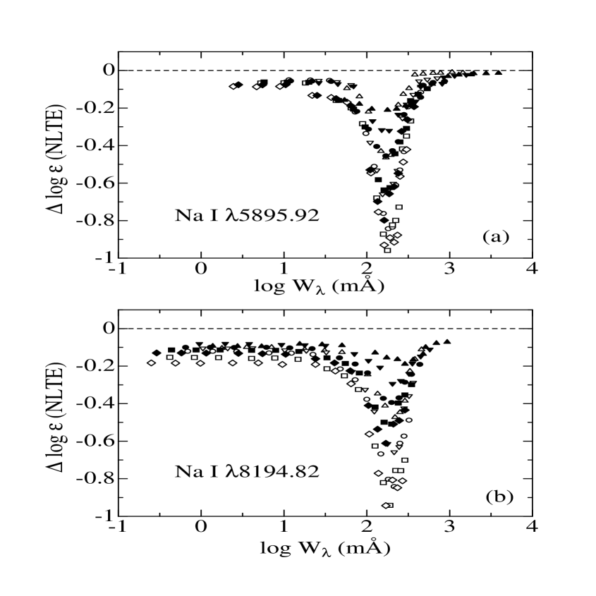
Figure 2: Theoretical non-LTE corrections as functions of the NLTE equivalent width for representative models, based on the electronic tables E1 (see subsection 2.3 for details). Different symbols discern the effective temperature (triangle, inverse triangle, circle, square, and diamond correspond to $T_{\rm eff}$ = 4500, 5000, 5500, 6000, and 6500 K, respectively) and the surface gravity (open and closed symbols are for $\log g$ = 2 and 4, respectively) of the adopted model atmospheres. The results derived for five different model-metallicities ([Fe/H] = 0, $-1$, $-2$, $-3$, and $-4$), while using the metallicity-scaled sodium abundance along with perturbations of $\pm 0.3$ dex, are shown here (though the same symbols are used for different metallicities/abundances). (a) Na i 5895.92. (b) Na i 8194.82.

2.3 Grid of Non-LTE Corrections

Based on the results of these calculations, we computed extensive grids of the theoretical equivalent-widths and the corresponding non-LTE corrections for the considered eight lines (Na i 5683, 5688, 5890, 5896, 6154, 6161, 8183, and 8195) for each of the model atmospheres as follows.

For an assigned sodium abundance ($A^{\rm a}$) and microturbulence ($\xi^{\rm a}$), we first calculated the non-LTE equivalent width ($W^{\rm NLTE}$) of the line by using the computed non-LTE departure coefficients ($b$) for each model atmosphere. Next, the LTE ($A^{\rm L}$) and NLTE ($A^{\rm N}$) abundances were computed from this $W^{\rm NLTE}$ while regarding it as if being a given observed equivalent width. We can then obtain the non-LTE abundance correction, $\Delta$, which is defined in terms of these two abundances as $\Delta\equiv A^{\rm N}-A^{\rm L}$.

Strictly speaking, the departure coefficients [$b(\tau)$] for a model atmosphere are applicable only to the case of the sodium abundance ($\log\epsilon_{\rm Na}^{\rm input}$) and the microturbulence (2 km s^-1) adopted in the non-LTE calculations (cf. subsection 2.1). Nevertheless, considering the fact that the departure coefficients (i.e., ratios of NLTE to LTE number populations) are (unlike the population itself) not much sensitive to small changes in atmospheric parameters, we also applied such computed $b$ values to evaluating $\Delta$ for slightly different $A^{\rm a}$ and $\xi^{\rm a}$ from those fiducial values assumed in the statistical equilibrium calculations. Hence, we evaluated $\Delta$ for three $A^{\rm a}$ values ($\log\epsilon_{\rm Na}^{\rm input}$ and $\pm 0.3$ dex perturbation) as well as three $\xi$ values (2 km s^-1 and $\pm 1$ km s^-1 perturbation) for a model atmosphere using the same departure coefficients.

We used the WIDTH9 program (Kurucz 1993a), which had been modified to incorporate the non-LTE departure in the line source function as well as in the line opacity, for calculating the equivalent width for a given abundance, or inversely evaluating the abundance for an assigned equivalent width . The adopted line data ($gf$ values, radiation damping constants, etc.) are given in table 1.

Table 1: Adopted atomic data of the Na i lines.

Mult.	Line	$\lambda$	$\chi$	$\log gf$	$\Gamma_{\rm R}$
1	$\lambda$5890	5889.95	0.00	+0.12	0.62
1	$\lambda$5896	5895.92	0.00	$-0.18$	0.62
4	$\lambda$8183	8183.26	2.10	+0.22	1.13
4	$\lambda$8195	8194.82	2.10	+0.52	1.13
5	$\lambda$6154	6154.23	2.10	$-1.56$	0.75
5	$\lambda$6161	6160.75	2.10	$-1.26$	0.75
6	$\lambda$5683	5682.63	2.10	$-0.67$	0.81
6	$\lambda$5688	5688.21	2.10	$-0.37$	0.81

Notes. Each of the columns 1–6 give the multiplet number, the line abbreviation used in this paper, the line wavelength (in $\rm\AA$), the lower excitation potential (in eV) , the logarithm of the $gf$ value, and the radiation damping constant in unit of $10^{8}$ s^-1. The data presented here are based on table 1 of Takeda and Takada-Hidai (1994), who consulted the compilation of Wiese et al. (1969). Each line was treated as if it is a single line, while neglecting any hyperfine structure (cf. subsection 2.3). See also subsection 2.3 for the treatment of the quadratic Stark effect damping and of the van der Waals effect damping.

One of the controversial factors in abundance determinations for late-type stars is the choice of the van der Waals effect damping constant. Regarding this parameter, we assumed the classical Unsöld’s (1955) formula unchanged, which means the adoption of $\Delta\log C_{6}=0.0$ ($C_{6}$ is connected to the damping width as $\log\Gamma_{6}=\log\Gamma_{6}^{\rm classical}+0.4\Delta\log C_{6}$). While this choice is based on our previous empirical investigations (cf. appendix A of Takeda, Takada-Hidai 1994; subsection 4.2 of Takeda 1995), we actually confirmed that this choice is reasonable from the analysis of solar Na i lines (cf. subsection 4.2). Anyhow, the precise value of this correction is not very essential unless very strong lines are used, as can be seen from figure 3 where the abundance changes expected by using $\Delta\log C_{6}=0.5$ are graphically displayed. Namely, the maximum change is $\sim 0.4|\Delta\log C_{6}|$ at most occurring only in the case of very strong damping-dominated lines and the low-temperature condition where $\Gamma_{6}$ dominates $\Gamma$ ($\equiv\Gamma_{\rm R}+\Gamma_{4}+\Gamma_{6}$). Regarding the quadratic Stark effect damping ($\Gamma_{4}$, which is comparatively insignificant in late-type stars), we followed the Peytremann’s formula (Kurucz 1979, p.8).

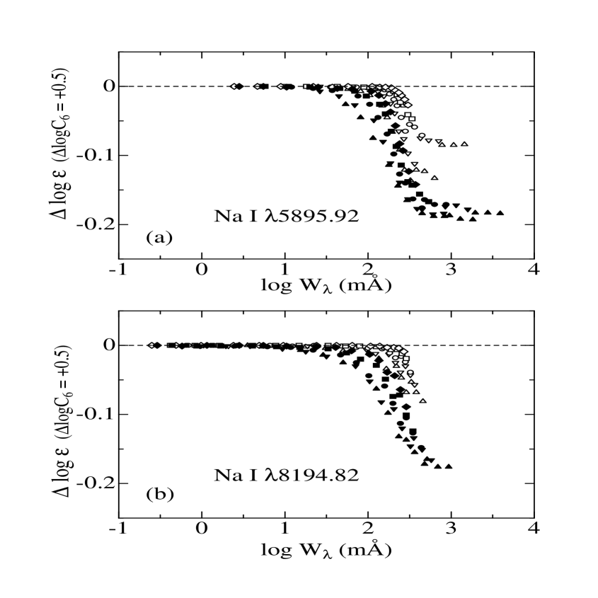
Figure 3: Differences of the resulting non-LTE abundances, when $\Delta\log C_{6}=+0.5$ (logarithmic correction applied to classical value of the van der Waals effect damping parameter) was used instead of the fiducial value of $\Delta\log C_{6}=0.0$, as functions of the non-LTE equivalent widths for the representative cases shown in table 2. See the caption of figure 2 for the meanings of the symbols. (a) Na i 5895.92. (b) Na i 8194.82.

Note also that we neglected the hyperfine structure (hfs; see, e.g., table 4 of McWilliam et al. 1995b for the 5890/5896 lines, and table 1 of Takeda, Takada-Hidai 1994 for the 8195 line) while treating each line as being purely single, because of a technical reason. However, this does not make any serious affection (several hundredths dex in most cases of actual importance) as illustrated in figure 4.

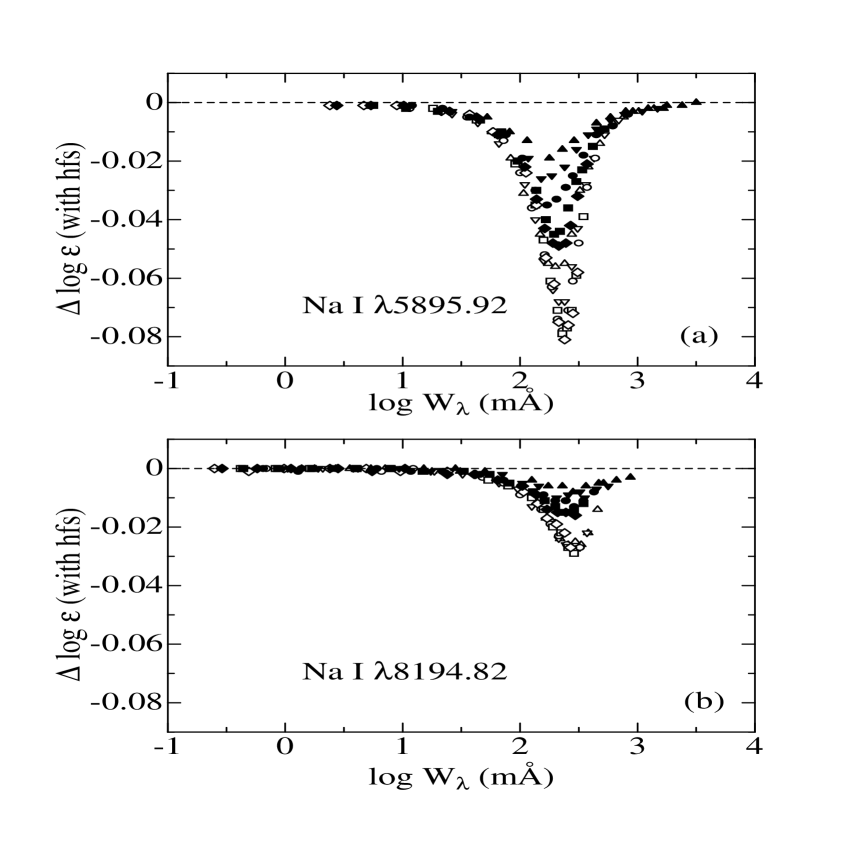
Figure 4: Differences of the resulting non-LTE abundances, when the hyperfine structure was approximately included instead of the purely single-line treatment (as basically adopted in this study; cf. table 1), as functions of the non-LTE equivalent widths for the representative cases shown in table 2. See the caption of figure 2 for the meanings of the symbols. (a) Na i $\lambda$5896 [using the two-component approximation of $gf(5895.93)=0.269$ and $gf(5895.95)=0.376$; cf. McWilliam et al. 1995b]. (b) Na i $\lambda$8195 [using the two-component approximation of $gf(8194.79)=0.332$ and $gf(8194.82)=2.999$; cf. Wiese et al. 1969].

As a demonstrative example of non-LTE corrections, we give the $\xi$ = 1 km s^-1 results for the Na i 5896 and 8195 lines computed for representative parameters [chosen to be nearly compatible with Baumüller et al.’s (1998) calculations] in table 2, where we also present the cases of $h=0,-2,-3$ in addition to the fiducial $h=-1$ case ($h$ is the logarithmic H i collision correction) for a comparison. Comparing this table 2 with Baumüller et al.’s (1998) table 2 (where they adopted $10^{h}=0.05$ or $h=-1.3$), we can see that our $|\Delta|$ values are quantitatively somewhat larger than theirs, though the qualitative tendency is in good agreement. The complete results (for all combinations of $T_{\rm eff}$, $\log g$, $\xi$ values for each of the 8 lines, though only for the fiducial case of $h=-1$) are available only in the electronic form. These tables (named “tables E1”) are temporarily at the anonymous ftp site of

ftp://www.ioa.s.u-tokyo.ac.jp/Users/takeda/sodium_paper/
(IP address: 133.11.160.242)

but will be replaced to CDS when the paper is to be published.

Table 2: Dependence of the non-LTE effect on the choice of the correction factor for the H i collision.

$T_{\rm eff}$	$\log g$	[Fe/H]	$\xi$	$A^{\rm a}$	$\lambda$	$W_{0}$	$W_{-1}$	$W_{-2}$	$W_{-3}$	$\Delta_{0}$	$\Delta_{-1}$	$\Delta_{-2}$	$\Delta_{-3}$
5500	4.0	0.0	1.0	6.33	5895.92	602.6	616.6	616.6	631.0	$-$0.04	$-$0.06	$-$0.06	$-$0.06
5500	4.0	$-$1.0	1.0	5.33	5895.92	309.0	316.2	331.1	331.1	$-$0.10	$-$0.15	$-$0.17	$-$0.18
5500	4.0	$-$2.0	1.0	4.33	5895.92	158.5	173.8	177.8	177.8	$-$0.26	$-$0.37	$-$0.40	$-$0.41
5500	4.0	$-$3.0	1.0	3.33	5895.92	85.1	89.1	91.2	89.1	$-$0.24	$-$0.33	$-$0.35	$-$0.33
5500	4.0	$-$4.0	1.0	2.33	5895.92	20.0	20.9	21.4	20.9	$-$0.03	$-$0.06	$-$0.06	$-$0.05
6500	4.0	0.0	1.0	6.33	5895.92	263.0	269.1	275.4	275.4	$-$0.18	$-$0.21	$-$0.21	$-$0.22
6500	4.0	$-$1.0	1.0	5.33	5895.92	169.8	177.8	182.0	182.0	$-$0.47	$-$0.55	$-$0.56	$-$0.56
6500	4.0	$-$2.0	1.0	4.33	5895.92	109.7	114.8	114.8	114.8	$-$0.61	$-$0.71	$-$0.72	$-$0.72
6500	4.0	$-$3.0	1.0	3.33	5895.92	38.0	39.8	39.8	38.9	$-$0.13	$-$0.16	$-$0.16	$-$0.16
6500	4.0	$-$4.0	1.0	2.33	5895.92	5.1	5.4	5.4	5.4	$-$0.06	$-$0.08	$-$0.08	$-$0.08
5500	4.0	0.0	1.0	6.33	8194.82	295.1	309.0	316.2	316.2	$-$0.15	$-$0.20	$-$0.21	$-$0.22
5500	4.0	$-$1.0	1.0	5.33	8194.82	154.9	173.8	182.0	186.2	$-$0.20	$-$0.35	$-$0.42	$-$0.44
5500	4.0	$-$2.0	1.0	4.33	8194.82	57.5	66.1	69.2	70.8	$-$0.08	$-$0.20	$-$0.25	$-$0.26
5500	4.0	$-$3.0	1.0	3.33	8194.82	10.0	11.8	12.3	12.3	$-$0.03	$-$0.10	$-$0.13	$-$0.13
5500	4.0	$-$4.0	1.0	2.33	8194.82	1.1	1.3	1.4	1.4	$-$0.03	$-$0.10	$-$0.12	$-$0.12
6500	4.0	0.0	1.0	6.33	8194.82	199.5	213.8	213.8	218.8	$-$0.34	$-$0.43	$-$0.47	$-$0.47
6500	4.0	$-$1.0	1.0	5.33	8194.82	107.2	117.5	123.0	123.0	$-$0.38	$-$0.55	$-$0.60	$-$0.61
6500	4.0	$-$2.0	1.0	4.33	8194.82	34.7	38.0	38.9	38.9	$-$0.12	$-$0.19	$-$0.21	$-$0.21
6500	4.0	$-$3.0	1.0	3.33	8194.82	4.9	5.5	5.6	5.6	$-$0.09	$-$0.13	$-$0.14	$-$0.14
6500	4.0	$-$4.0	1.0	2.33	8194.82	0.5	0.6	0.6	0.6	$-$0.09	$-$0.13	$-$0.14	$-$0.14

Notes. Columns 1–6 are self-explanatory (the units of $T_{\rm eff}$, $g$, and $\xi$ are K, cm s^-2, and km s^-1, respectively). The suffixes ($0$, $-1$, $-2$, $-3$, and $-4$) appended to $W$ (the non-LTE equivalent width in m$\rm\AA$ calculated for the atmospheric parameters and the assigned sodium abundance given in columns 1–5) and $\Delta$ (the non-LTE abundance correction) denote the corresponding values of $h$ (the logarithm of the H i collision correction factor applied to the classical formula).

3 Observational Data

Our observational data consist of those obtained at two observatories, Beijing Astronomical Observatory (BAO; 2.2 m reflector + coude echelle spectrograph at Xinglong station) in P. R. China and Okayama Astrophysical Observatory (OAO; 1.9 m reflector + coude HIgh-Dispersion Echelle Spectrograph named “HIDES”) in Japan.

3.1 BAO Data

The BAO spectra ($R\sim 40000$ and S/N $\sim$ 200–400) used here are such those originally collected for the purpose of Chen et al.’s (2000) comprehensive analyses on Galactic disk stars. See subsection 2.2 therein for detailed information on the observations and the data quality. Chen et al. (2000) determined the abundance of sodium based on the comparatively weak Na i 6154/6161 lines, though the used equivalent-widths data were not published. For the present study, additional measurements for five lines (Na i 5683, 5688, 5890, 5896, and 8195; the 8183 line was discarded because of the contamination of telluric lines) were newly carried out by one of us (Y.-Q. Chen; cf. subsection 2.3 of Chen et al. 2000 for the measurement method) on the spectra of 22 F–G stars (+ Moon), which are our BAO program stars also adopted in our previous potassium analysis (Takeda et al. 2002). Although many lines (except for the 6154/6161 lines) are so strong in these disk stars and not suitable for sodium abundance determinations, we tried to derive the abundances from them in order to see whether the similar behavior of [Na/Fe] may be reproduced among the different line groups (cf. subsection 5.2). Yet, it should be kept in mind that difficulties are involved in measuring the equivalent widths of very strong damping-dominated lines such as the 5890/5896 D lines, with which errors are more or less involved. Nevertheless, comparing the solar (Moon) equivalent width measured by us with those taken from the literature (cf. table 3), we can see that our measurements are regarded as being reasonable (i.e., crucial systematic discrepancies are not observed). The finally obtained BAO equivalent-widths are given in tables 4 and 5.

Table 3: Comparison of the solar equivalent widths (in m$\rm\AA$) of Na i lines taken from various literature.

Ref.	$\lambda$5683	$\lambda$5688	$\lambda$5890	$\lambda$5896	$\lambda$6154	$\lambda$6161	$\lambda$8183	$\lambda$8195	Data source
(1)	100.4	131.1	837.2	545.0	38.6	59.5	$\cdots$	306.1	BAO Moona
(2)	105.3	128.6	$\cdots$	$\cdots$	$\cdots$	$\cdots$	$\cdots$	$\cdots$	B76 solar flux
(3)	106.9	127.9	$\cdots$	$\cdots$	$\cdots$	$\cdots$	$\cdots$	$\cdots$	B76 solar flux
(4)	106.9	127.9	$\cdots$	$\cdots$	36.8	58.6	$\cdots$	$\cdots$	B76 solar flux
(5)	$\cdots$	129.0	1125.5	736.5	$\cdots$	$\cdots$	257.3	326.6	solar flux & disk centerb
(6)	$\cdots$	$\cdots$	$\cdots$	$\cdots$	35.0	53.7	$\cdots$	$\cdots$	solar disk centerc
(7)	90.0	119.1	$\cdots$	$\cdots$	40.5	58.2	$\cdots$	$\cdots$	K84 solar flux
(8)	121	144	830	640	41	63	254	328	K84 solar flux
(9)	$\cdots$	$\cdots$	756	597	$\cdots$	$\cdots$	244	315	K84 solar fluxd
(10)	103.0	128.0	$\cdots$	$\cdots$	36.0	$\cdots$	$\cdots$	$\cdots$	From (12)?
(11)	$\cdots$	$\cdots$	$\cdots$	$\cdots$	38.6	59.5	$\cdots$	$\cdots$	K84 solar flux
(12)	103	128	765	570	36	53	239	322	solar disk centere

References: (1) This study; (2) Peterson and Carney (1979); (3) Peterson (1980); (4) Peterson (1981); (5) Gratton and Sneden (1987b); (6) Tomkin et al. (1985); (7) Prochaska et al. (2000); (8) Mashonkina et al. (2000); (9) Takeda (1995); (10) Carretta et al. (2000); (11) Sadakane et al. (2002); (12) Holweger (1971).

Notes on the data sources:
B76 and K84 means the solar flux spectrum atlas published by Beckers et al. (1976) and Kurucz et al. (1984), respectively.
^a Moon spectrum observed at Beijing Astronomical Observatory.
^b Based on two different atlases (see Gratton, Sneden 1987a).
^c Taken from the values published by Lambert and Luck (1978), which are based on two different atlases.
^d Inversely computed from the profile fitting solutions.
^e Based on three different atlases.

Table 4: Analysis of Na i 8183/8195 lines based on the BAO and OAO data.

Star	Sp. type	$T_{\rm eff}$	$\log g$	[Fe/H]	$\xi$	$W_{8183}$	$A^{\rm N}_{8183}$	$\Delta_{8183}$	$W_{8195}$	$A^{\rm N}_{8195}$	$\Delta_{8195}$	Ref.
[BAO sample]
Sun	G2 V	5780	4.44	0.00	1.0	$\cdots$	$\cdots$	$\cdots$	306.1	6.32	$-$0.19	(1)
HD 010307	G1.5 V	5776	4.13	$-$0.05	1.8	$\cdots$	$\cdots$	$\cdots$	265.5	6.08	$-$0.31	(1)
HD 019373	G0 V	5867	4.01	+0.03	1.8	$\cdots$	$\cdots$	$\cdots$	274.8	6.23	$-$0.32	(1)
HD 022484	F9 IV-V	5915	4.03	$-$0.13	2.0	$\cdots$	$\cdots$	$\cdots$	242.5	5.97	$-$0.39	(1)
HD 034411	G1.5 IV-V	5773	4.02	+0.01	1.7	$\cdots$	$\cdots$	$\cdots$	275.8	6.20	$-$0.30	(1)
HD 039587	G0 V	5805	4.29	$-$0.18	2.2	$\cdots$	$\cdots$	$\cdots$	273.9	5.99	$-$0.32	(1)
HD 041640	F5	6004	4.37	$-$0.62	2.0	$\cdots$	$\cdots$	$\cdots$	205.6	5.65	$-$0.39	(1)
HD 049732	F8	6260	4.15	$-$0.70	1.9	$\cdots$	$\cdots$	$\cdots$	178.3	5.63	$-$0.50	(1)
HD 055575	G0 V	5802	4.36	$-$0.36	1.6	$\cdots$	$\cdots$	$\cdots$	$\cdots$	$\cdots$	$\cdots$	(1)
HD 060319	F8	5867	4.24	$-$0.85	1.6	$\cdots$	$\cdots$	$\cdots$	171.4	5.41	$-$0.39	(1)
HD 062301	F8 V	5837	4.23	$-$0.67	1.7	$\cdots$	$\cdots$	$\cdots$	190.1	5.53	$-$0.38	(1)
HD 068146	F7 V	6227	4.16	$-$0.09	2.1	$\cdots$	$\cdots$	$\cdots$	229.4	6.01	$-$0.42	(1)
HD 069897	F6 V	6243	4.28	$-$0.28	2.0	$\cdots$	$\cdots$	$\cdots$	197.5	5.77	$-$0.42	(1)
HD 076349	G0	6004	4.21	$-$0.49	2.1	$\cdots$	$\cdots$	$\cdots$	210.9	5.69	$-$0.43	(1)
HD 101676	F6 V	6102	4.09	$-$0.47	2.0	$\cdots$	$\cdots$	$\cdots$	214.8	5.82	$-$0.47	(1)
HD 106516	F5 V	6135	4.34	$-$0.71	1.5	$\cdots$	$\cdots$	$\cdots$	168.6	5.55	$-$0.41	(1)
HD 109303	F8	5905	4.10	$-$0.61	1.7	$\cdots$	$\cdots$	$\cdots$	186.5	5.56	$-$0.43	(1)
HD 118244	F5 V	6234	4.13	$-$0.55	2.3	$\cdots$	$\cdots$	$\cdots$	197.7	5.68	$-$0.50	(1)
HD 142373	F8 Ve	5920	4.27	$-$0.39	1.5	$\cdots$	$\cdots$	$\cdots$	$\cdots$	$\cdots$	$\cdots$	(1)
HD 142860	F6 IV	6227	4.18	$-$0.22	2.2	$\cdots$	$\cdots$	$\cdots$	211.5	5.84	$-$0.44	(1)
HD 167588	F8 V	5894	4.13	$-$0.33	1.7	$\cdots$	$\cdots$	$\cdots$	$\cdots$	$\cdots$	$\cdots$	(1)
HD 201891	F8 V-IV	5827	4.43	$-$1.04	1.6	$\cdots$	$\cdots$	$\cdots$	152.6	5.21	$-$0.33	(1)
HD 208906	F8 V-IV	5929	4.39	$-$0.73	1.5	$\cdots$	$\cdots$	$\cdots$	173.9	5.47	$-$0.36	(1)
[OAO sample]
HD 6833	G9 III	4450	1.40	$-$0.90	1.6	161.3	4.92	$-$0.41	207.9	5.10	$-$0.46	(2)
HD 26297	G5/G6 Ivw	4500	1.20	$-$1.60	1.7	86.4	4.24	$-$0.21	115.6	4.24	$-$0.32	(2)
HD 73394	G5 IIIw	4500	1.10	$-$1.40	1.5	127.7	4.71	$-$0.37	157.0	4.73	$-$0.46	(3)
HD 76932	F7/F8 IV/V	5900	4.12	$-$0.80	1.3	125.1	5.40	$-$0.38	155.6	5.37	$-$0.42	(4)a
HD 88609	G5 IIIw	4570	0.75	$-$2.70	1.9	10.8	3.18	$-$0.10	20.1	3.19	$-$0.11	(4)
HD 106516	F5 V	6200	4.31	$-$0.70	1.1	134.8	5.66	$-$0.41	167.1	5.65	$-$0.42	(4)a
HD 108317	G0	5300	2.90	$-$2.24	1.0	26.5	3.95	$-$0.16	41.0	3.91	$-$0.18	(5)
HD 122563	F8 IV	4590	1.17	$-$2.74	2.3	15.7	3.35	$-$0.11	31.5	3.41	$-$0.12	(6)
HD 140283	sdF3	5690	3.69	$-$2.42	0.8	6.0	3.38	$-$0.12	9.6	3.29	$-$0.13	(7)a
HD 165908	F7 V	5900	4.09	$-$0.60	1.7	143.2	5.51	$-$0.39	179.9	5.51	$-$0.43	(4)
HD 167588	F8 V	5890	4.13	$-$0.33	1.7	170.9	5.76	$-$0.38	205.3	5.72	$-$0.39	(1)
HD 187111	G8wvar	4260	0.51	$-$1.85	1.8	94.5	4.18	$-$0.19	147.6	4.41	$-$0.34	(6)
HD 189322	G8 III	4464	2.00	$-$1.57	2.0	222.1	5.37	$-$0.43	260.0	5.38	$-$0.38	(8)b
HD 216143	G5	4525	1.00	$-$2.10	2.9	50.0	3.86	$-$0.12	70.7	3.78	$-$0.15	(2)
HD 221170	G2 IV	4425	1.00	$-$2.15	1.5	53.0	3.91	$-$0.14	79.4	3.93	$-$0.20	(5)
BD +37∘1458	G0	5200	3.00	$-$2.00	1.3	19.8	3.73	$-$0.15	42.7	3.86	$-$0.18	(2)
Procyon	F5 IV-V	6510	3.96	$-$0.05	2.2	188.7	6.14	$-$0.51	220.3	6.08	$-$0.53	(9)

Notes. Columns 1–6 are self-explanatory as in table 2. $W$ is the observed equivalent width (in m$\rm\AA$), $A^{\rm N}$ is the logarithmic non-LTE abundance (in the usual normalization of H = 12), and $\Delta$ is the non-LTE correction ($\equiv A^{\rm N}-A^{\rm L}$), respectively. Column 13 gives the keys to the references of the atmospheric parameters (cf. subsection 4.1): (1) Chen et al. (2000);(2) Fulbright (2000); (3) Luck and Bond (1985);(4) Takada-Hidai et al. (2002); (5) Pilachowski et al. (1996); (6) Gratton and Sneden (1994); (7) Nissen et al. (2002); (8) Alonso et al. (1999); (9) Allende Prieto et al. (2002).
^a Only the $\xi$ value was taken from (2).
^b The $\xi$ value was assumed.

Table 5: Analysis of Na i 5683/5688, 5890/5896, and 6154/6160 lines based on the BAO data.

Star	$W_{5683}$	$A^{\rm N}_{5683}$	$\Delta_{5683}$	$W_{5688}$	$A^{\rm N}_{5688}$	$\Delta_{5688}$	$W_{5890}$	$A^{\rm N}_{5890}$	$\Delta_{5890}$	$W_{5896}$	$A^{\rm N}_{5896}$	$\Delta_{5896}$	$W_{6154}$	$A^{\rm N}_{6154}$	$\Delta_{6154}$	$W_{6161}$	$A^{\rm N}_{6161}$	$\Delta_{6161}$
[BAO sample]
Sun	100.4	6.28	$-$0.11	131.1	6.33	$-$0.13	837.2	6.41	$-$0.05	545.0	6.27	$-$0.07	38.6	6.31	$-$0.04	59.5	6.32	$-$0.06
HD 010307	$\cdots$	$\cdots$	$\cdots$	134.3	6.26	$-$0.16	779.2	6.43	$-$0.07	506.5	6.30	$-$0.09	39.4	6.29	$-$0.05	60.6	6.28	$-$0.07
HD 019373	$\cdots$	$\cdots$	$\cdots$	139.6	6.39	$-$0.19	$\cdots$	$\cdots$	$\cdots$	$\cdots$	$\cdots$	$\cdots$	45.8	6.44	$-$0.05	65.3	6.40	$-$0.07
HD 022484	$\cdots$	$\cdots$	$\cdots$	116.9	6.12	$-$0.17	458.5	6.02	$-$0.12	402.6	6.16	$-$0.13	32.1	6.23	$-$0.06	47.1	6.17	$-$0.07
HD 034411	$\cdots$	$\cdots$	$\cdots$	133.6	6.30	$-$0.17	795.3	6.52	$-$0.07	505.6	6.37	$-$0.08	39.7	6.30	$-$0.05	65.6	6.36	$-$0.07
HD 039587	$\cdots$	$\cdots$	$\cdots$	118.1	6.01	$-$0.13	625.6	6.11	$-$0.09	459.5	6.06	$-$0.12	24.0	6.01	$-$0.05	48.4	6.11	$-$0.06
HD 041640	$\cdots$	$\cdots$	$\cdots$	77.2	5.69	$-$0.12	413.1	5.69	$-$0.16	316.3	5.64	$-$0.21	9.1	5.63	$-$0.07	21.8	5.75	$-$0.07
HD 049732	$\cdots$	$\cdots$	$\cdots$	73.7	5.78	$-$0.15	343.8	5.80	$-$0.24	260.8	5.65	$-$0.34	7.7	5.65	$-$0.08	17.3	5.74	$-$0.09
HD 055575	$\cdots$	$\cdots$	$\cdots$	93.2	5.82	$-$0.12	$\cdots$	$\cdots$	$\cdots$	412.6	5.90	$-$0.11	21.6	5.96	$-$0.05	36.2	5.95	$-$0.06
HD 060319	$\cdots$	$\cdots$	$\cdots$	59.7	5.45	$-$0.11	354.5	5.42	$-$0.18	270.9	5.36	$-$0.23	6.3	5.40	$-$0.07	17.8	5.60	$-$0.08
HD 062301	$\cdots$	$\cdots$	$\cdots$	71.8	5.58	$-$0.12	407.8	5.60	$-$0.14	285.8	5.43	$-$0.21	10.2	5.61	$-$0.07	19.9	5.64	$-$0.07
HD 068146	$\cdots$	$\cdots$	$\cdots$	115.9	6.24	$-$0.17	436.3	6.19	$-$0.15	352.0	6.20	$-$0.18	24.6	6.23	$-$0.06	43.3	6.25	$-$0.07
HD 069897	$\cdots$	$\cdots$	$\cdots$	94.1	6.01	$-$0.14	374.0	5.92	$-$0.18	306.3	5.92	$-$0.23	14.5	5.96	$-$0.06	29.1	6.02	$-$0.07
HD 076349	$\cdots$	$\cdots$	$\cdots$	87.1	5.79	$-$0.14	401.0	5.74	$-$0.17	318.0	5.71	$-$0.22	14.7	5.85	$-$0.07	29.8	5.92	$-$0.08
HD 101676	$\cdots$	$\cdots$	$\cdots$	93.0	5.93	$-$0.16	$\cdots$	$\cdots$	$\cdots$	294.5	5.76	$-$0.27	15.3	5.92	$-$0.07	31.2	5.99	$-$0.08
HD 106516	$\cdots$	$\cdots$	$\cdots$	69.9	5.71	$-$0.13	313.5	5.52	$-$0.21	260.6	5.56	$-$0.26	9.0	5.68	$-$0.07	22.1	5.82	$-$0.08
HD 109303	$\cdots$	$\cdots$	$\cdots$	78.6	5.70	$-$0.14	382.4	5.66	$-$0.17	279.4	5.53	$-$0.23	8.1	5.53	$-$0.07	32.2	5.93	$-$0.08
HD 118244	$\cdots$	$\cdots$	$\cdots$	91.9	5.93	$-$0.16	353.7	5.78	$-$0.25	281.9	5.68	$-$0.34	9.7	5.75	$-$0.08	29.5	6.00	$-$0.09
HD 142373	68.1	5.89	$-$0.10	$\cdots$	$\cdots$	$\cdots$	407.0	5.75	$-$0.12	401.1	6.03	$-$0.13	12.6	5.75	$-$0.06	26.5	5.84	$-$0.07
HD 142860	$\cdots$	$\cdots$	$\cdots$	106.3	6.11	$-$0.16	449.6	6.18	$-$0.16	317.6	5.98	$-$0.24	17.6	6.05	$-$0.06	44.0	6.25	$-$0.08
HD 167588	75.1	5.96	$-$0.11	97.4	5.92	$-$0.15	423.4	5.84	$-$0.13	368.4	5.96	$-$0.14	19.1	5.95	$-$0.06	37.6	6.02	$-$0.07
HD 201891	$\cdots$	$\cdots$	$\cdots$	43.3	5.20	$-$0.09	328.1	5.14	$-$0.19	209.3	4.82	$-$0.28	7.4	5.46	$-$0.07	9.6	5.28	$-$0.07
HD 208906	52.1	5.68	$-$0.09	$\cdots$	$\cdots$	$\cdots$	$\cdots$	$\cdots$	$\cdots$	$\cdots$	$\cdots$	$\cdots$	9.2	5.61	$-$0.07	21.3	5.72	$-$0.07

See the notes to table 4 for the meanings of the $W$, $A^{\rm N}$, and $\Delta$.

3.2 OAO Data

The OAO data are based on the near-IR spectra of 17 mostly metal-poor disk/halo stars (dwarfs and giants being mixed), which have been collected by using HIDES during our observing runs in 2001–2002. The slit width of 250 $\mu$m ($0.^{\prime\prime}95$) was set to yield a spectral resolution of $R\sim 50000$. By using the single 4K$\times$2K CCD (pixel size of 13.5 $\mu$m $\times$ 13.5 $\mu$m), a wavelength span of $\sim 1100\;\rm\AA$ could be covered at one time. Most of our observations were made in the wavelength region of $\sim$ 7700–8800 $\rm\AA$.

The data reduction was performed with the IRAF echelle package, following the standard procedure for extracting one-dimensional spectra. We also removed the telluric lines using the telluric task of IRAF and the spectra of a rapid rotator. The S/N ratios of the resulting spectra, differing from star to star, are typically of the order of 200–300. The resulting OAO equivalent widths of the Na i 8183/8195 lines based on these spectra, which were measured by the Gaussian fitting or direct integration method using the splot task of IRAF, are presented in table 4. Note that, although two stars (HD 106516 and HD 167588) are common to BAO and OAO samples, they were treated independently.

4 Abundance Analyses

4.1 Atmospheric Parameters

First we need to establish the four atmospheric parameters [$T_{\rm eff}$ (effective temperature), $\log g$ (surface gravity), [Fe/H] (metallicity; represented by the Fe abundance relative to the Sun), and $\xi$ (microturbulent velocity dispersion)], which are necessary for constructing the model atmosphere and deriving the abundance from an equivalent width. Regarding the 22 BAO stars, the parameter data determined by Chen et al. (2000) were used unchanged, while the reasonably known solar parameters of (5780 K, 4.44, 0.0, 1.0 km s^-1) were applied to the analysis of the BAO Moon data. Meanwhile, the atmospheric parameters of 17 OAO stars were taken from the published values found in various literature (cf. column 13 of table 4); when two or more references were available for the same star, we selected an appropriate value according to our personal judgment. The finally adopted values are given in table 4.

As for the model atmospheres, Kurucz’s (1993a) grid of ATLAS9 models was used as in the case of non-LTE calculations, based on which the model of each star was obtained by a three-dimensional interpolation with respect to $T_{\rm eff}$, $\log g$, and [Fe/H]. Similarly, the depth-dependent departure coefficients ($b$) of Na i levels computed for the grid of models (cf. section 2) were interpolated in terms of $T_{\rm eff}$, $\log g$, and [Fe/H], in order to evaluate the $S_{\rm L}(\tau)/B(\tau)$ and $l_{0}^{\rm NLTE}(\tau)/l_{0}^{\rm LTE}(\tau)$ ratios for each star.

4.2 Abundance Determination

The procedures for determining the sodium abundances from the equivalent widths of Na i lines are the same as already explained in subsection 2.3 (i.e., modified WIDTH9 program, line data given in table 1, $\Delta\log C_{6}=0$, neglecting the hfs effect).

The resulting non-LTE abundance ($A^{\rm N}$) and the non-LTE abundance correction ($\equiv A^{\rm N}-A^{\rm L}$) derived for each line and for each star are presented in tables 4 (8183/8195 lines) and 5 (5683/5688, 5890/5896, and 6154/6161 lines). As can be seen from these two tables, the solar non-LTE abundances derived from the BAO Moon equivalent widths of Na i 8195 (6.32), 5683 (6.28), 5688 (6.33), 5890 (6.41), 6154 (6.31), and 6160 (6.32) are in remarkable agreement with each other; moreover, their average of $6.32(\sigma=0.04)$ is essentially the same as the standard solar sodium abundance of 6.33 (Anders, Grevesse 1989). Accordingly, we confirmed the internal consistency of using $\Delta\log C_{6}=0.0$, as far as our present analysis using ATLAS9 model atmospheres is concerned. [Actually, empirical determination of this correction significantly depends on the choice of the atmospheric models, as demonstrated in subsection 4.2 of Takeda (1995).]

The abundance changes caused by uncertainties in the atmospheric parameters are quantitatively similar to the case of potassium described in section 5 of Takeda et al. (2002), since K and Na have quite similar atomic structures to each other (alkali atom with one valence electron; ionization potential of 4–5 eV) and most atoms are in the once-ionized stage. Hence, even for changes of $\Delta T_{\rm eff}\sim\pm 200$ K or $\Delta\log g\sim\pm 0.3$ dex (we expect that internal errors in the parameters of our program stars, especially for BAO sample stars, are smaller than these), the extents of the resulting abundance variations are $\mathrel{\hbox{\hbox to0.0pt{\hbox{\lower 4.0pt\hbox{$\sim$}}\hss}\hbox{$<$}}}0.2$ dex, as can be seen from table 1 of Takeda et al. (2002). The effect of changing the microturbulence, which influences only the lines at the flat part of the curve of growth ($W_{\lambda}\sim$ 100–300 m$\rm\AA$; cf. figure 4) can also be assessed by inspecting that table.

The [Na/Fe] ratios (Na-to-Fe logarithmic abundance ratio relative to the Sun) can be obtained based on the results in tables 4 and 5 as $A^{\rm N}({\rm star})-6.33-[{\rm Fe}/{\rm H}]$, where we assumed Anders and Grevesse’s (1989) value of 6.33 as the reference solar Na abundance. The resulting [Na/Fe] vs. [Fe/H] relations derived from each of the four multiplets, along with the corresponding non-LTE corrections, are displayed in figure 5.

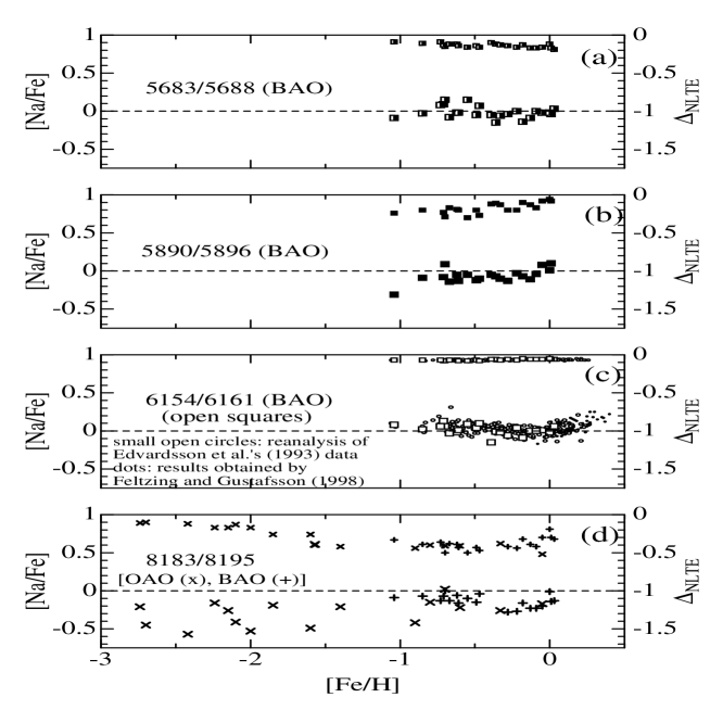
Figure 5: The [Na/Fe] values resulting from the non-LTE analysis of our BAO and OAO data (larger symbols; scale in the left-hand axis) and the corresponding non-LTE corrections (smaller symbols; scale in the right-hand axis), plotted as functions of [Fe/H]; these are based on the data presented in tables 4 and 5. (a) $\lambda$5683/$\lambda$5688 lines of multiplet 6, plotted in half-filled squares (BAO). (b) $\lambda$5890/$\lambda$5896 lines of multiplet 1, plotted in filled squares (BAO). (c) $\lambda$6154/$\lambda$6161 lines of multiplet 5, plotted in open squares (BAO). The results of our reanalysis of Edvardsson et al.’s (1993) data (also depicted in figure 7a) and the results of Feltzing and Gustafsson (1998) (the LTE [Na/Fe] values obtained by themselves; their equivalent-width data are not published) are also shown with small open circles and dots, respectively, for a comparison. (d) $\lambda$8183/$\lambda$8195 lines of multiplet 4, plotted in Greek crosses (BAO) and St. Andrew’s crosses (OAO), respectively.

Note that when two lines of the same multiplet are available, we averaged the abundances ([Na/Fe]) as well as the non-LTE corrections for both lines and such derived mean results for the multiplet are shown.

4.3 Literature Data Analysis

We also tried to reanalyze the published equivalent-width data (for the Na i 5683/5688, 5890/5896, 6154/6161, and 8183/8195 lines) of late-type stars in the Galactic disk as well as in the halo covering a wide range of metallicities, while taking account of the non-LTE effect. In searching for the papers including the observational data we need, the extensive references quoted by Timmes et al. (1995), Samland (1998), and Goswami and Prantzos (2000) were quite helpful. Although our literature survey is not complete, we consider that we have picked up most of the important works done after 1980’s.

These data were analyzed just in the same way as we did for our BAO/OAO data (cf. subsections 4.1 and 4.2). The atmospheric parameters were taken from the same paper as that presenting the equivalent-width data as far as possible. By inspecting those original papers, we found that abundance analyses done before 1990 tend to be based on rather coarsely determined parameters (e.g., using rounded $T_{\rm eff}$ or $\log g$ values; assuming the same $\xi$ values for all program stars, etc.) compared to the more recent studies carried out this decade. Accordingly, we decided to present the results of the reanalyzes on the data before and after 1990 separately. Figure 6 shows the resulting [Na/Fe] vs. [Fe/H] relations and the corresponding non-LTE corrections derived from the older data before 1990, while those obtained from the analyses of the recent data after 1990 are displayed in figure 7.

The same results as those in figure 7a (the reanalysis results based on the new data after 1990) are also depicted in figure 8a, where the [Na/Fe] data are plotted with a more compressed vertical scale (for the purpose of clarifying the global tendency) and low- and high-gravity stars are distinguished by different symbols. In addition, figure 8b shows the $T_{\rm eff}$ vs. $\log g$ plots relevant to these data; it can be seen from this figure that most of the high-gravity stars are comparatively higher $T_{\rm eff}$ stars of mid-F through late-G type, while low-gravity stars mainly consist of late-G through early-K giants of lower $T_{\rm eff}$ and show a positive correlation between $T_{\rm eff}$ and $\log g$ (reflecting the evolutionary sequence). We may state from an inspection of figure 8a that any meaningful systematic $\log g$-dependent difference does not exist in the [Na/Fe] values; however, the biased sample (i.e., very low-metallicity stars tend to be low-gravity giants, and vice versa) prevents us from making any definite argument regarding this point.

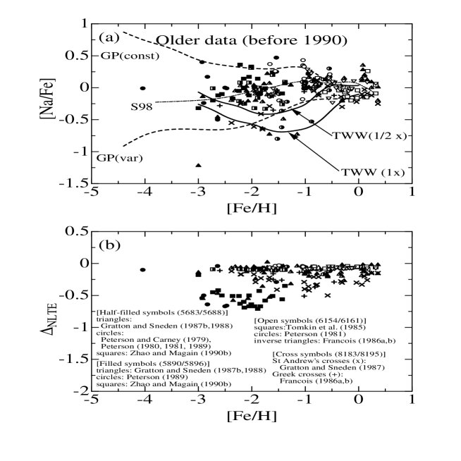
Figure 6: (a) [Na/Fe] vs. [Fe/H] relation resulting from the non-LTE reanalysis of the rather old data published before 1990. See panel (b) for the data sources of equivalent widths and the corresponding symbols. Lines show the representative theoretical predictions: Dash-dotted line (S98)— taken from figure 8 of Samland (1998), dashed line (TWW) — taken from figure 17 of Timmes et al. (1995) corresponding to the two cases for the standard Woosley and Weaver’s (1995) Fe yield from massive stars and the reduced one by a factor of 2 (which may be more reasonable according to their suggestion), dashed line — taken from figure 7 of Goswami and Prantzos (2000), for the two cases of Na yield; time-independent constant yield [GP(const); only for a comparison purpose] and the realistic metallicity-dependent Na yield [GP(var)]. (b) The corresponding NLTE corrections used for deriving the [Na/Fe] values shown in panel (a), plotted as functions of [Fe/H].

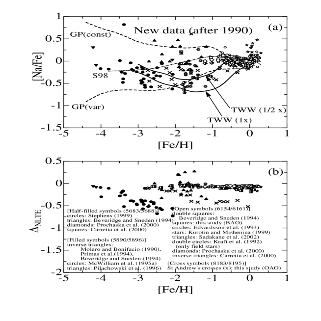
Figure 7: (a) [Na/Fe] vs. [Fe/H] relation resulting from the non-LTE reanalysis based on the recently published new data after 1990. The data point for CS 22949-037 ([Na/Fe] = +1.94 at [Fe/H] = $-3.99$) derived from the reanalysis of McWilliam et al.’s (1995a) EW data is outside the plot range of this figure (cf. figure 8a for a more global view including this anomalous point). (b) The corresponding NLTE corrections used for deriving the [Na/Fe] values shown in panel (a), plotted as functions of [Fe/H]. Otherwise, the same as in figure 6; see the caption therein for more details. The results of the reanalysis of Pilachowski et al.’s (1996) 5890/5896 data for the low-gravity giants/supergiants (filled triangles) may suffer rather large uncertainties and should not be seriously taken (cf. the footnote in subsection 5.3).

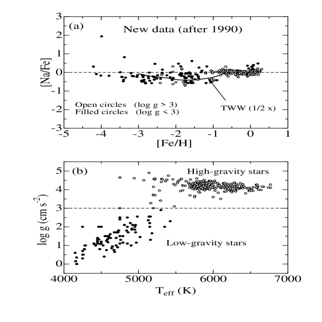
Figure 8: (a) [Na/Fe] vs. [Fe/H] relation resulting from the non-LTE reanalysis of the new literature data after 1990. The plotted data are essentially the same as in figure 7a, but dwarfs and giants are discriminated by different symbols: open circles — high-gravity stars ($\log g\geq 3$), filled clrcles — low-gravity stars ($\log g<3$). The theoretical prediction of Timmes et al. (1995) (the case of reduced Fe yield denoted by “TWW (1/2 $\times$)”; cf. the caption of figure 6a), which appears to match the observed trend most satisfactorily, is also drawn for a comparison. (b) $T_{\rm eff}$ vs. $\log g$ relation for the sample stars relevant to the data plots in (a). The meanings of the symbols as the same as in (a).

The details of these analyses (the data of the used equivalent widths and the adopted parameter values, the resulting non-LTE abundances or [Na/Fe] values with the non-LTE corrections, given for each line/multiplet and for each star) are available only electronically as “tables E2”(from the ftp site mentioned at the end of subsection 2.3).

5 Discussion

5.1 Non-LTE Effect

Figures 5, 6, and 7 clearly show how the non-LTE effect acts on different Na i lines in sodium abundance determinations for stars of various metallicities.

Roughly speaking, a simple principle appears to hold: The non-LTE effect (negative corrections to the corresponding LTE abundances) tends to be most important for rather strong saturated lines (with equivalent widths of 100–300 m$\rm\AA$) on the flat part of the curve of growth, and it becomes progressively insignificant towards decreasing strengths (i.e., unsaturated weak lines on the linear part) as well as increasing strengths (i.e., extremely strong damping-dominated lines in the damping part), reflecting the importance of the core-deepening effect caused by the dilution of $S_{\rm L}$ as already mentioned in subsection 2.2 (cf. figure 2).

This naturally explains the behaviors of the extent of the non-LTE corrections for each line at different metallicities; for example, the reason why the weak 6154/6161 lines in disk stars show almost negligible non-LTE effects (cf. figure 5c), why the $|\Delta|$ values for the 8183/8195 attain maximum at [Fe/H] $\sim-1$ (cf. figures 5d, 6b, and 7b), and why the $|\Delta|$ values for the 5890/5896 lines systematically decreases from [Fe/H] $\sim-2$ to $\sim-4$ (cf. figure 7b).

We should note, however, that the situation more or less differs from line to line, reflecting their individual properties. For example, lines at longer wavelengths tend to suffer larger non-LTE effects because of the decreasing sensitivity of the Planck function to the temperature (i.e., the minimum allowed LTE residual intensity tends to be raised and thus the difference between LTE and non-LTE becomes more significant). Hence, we can understand the fact that the near-IR 8183/8195 lines show relatively larger non-LTE effects compared to the other lines at similar line-strengths.

Based on figures 5–7, we can assess the importance of the non-LTE effect on different lines in sodium abundance determinations as follows: The 6154/6161 lines are the best abundance indicators, for which the non-LTE effect is practically insignificant (i.e., $\mathrel{\hbox{\hbox to0.0pt{\hbox{\lower 4.0pt\hbox{$\sim$}}\hss}\hbox{$<$}}}0.1$ dex) and may be neglected, though they are usable/visible only at $-2\mathrel{\hbox{\hbox to0.0pt{\hbox{\lower 4.0pt\hbox{$\sim$}}\hss}\hbox{$<$}}}$ [Fe/H] $\mathrel{\hbox{\hbox to0.0pt{\hbox{\lower 4.0pt\hbox{$\sim$}}\hss}\hbox{$<$}}}0.5$). The 5683/5688 lines may also be tolerably analyzed with LTE at the metallicity of $-3\mathrel{\hbox{\hbox to0.0pt{\hbox{\lower 4.0pt\hbox{$\sim$}}\hss}\hbox{$<$}}}$ [Fe/H] $\mathrel{\hbox{\hbox to0.0pt{\hbox{\lower 4.0pt\hbox{$\sim$}}\hss}\hbox{$<$}}}-1$. Regarding the 5890/5896 and 8183/8195 lines, which are important for diagnosing the Na abundance behaviors of very metal-deficient stars because of their strengths (especially, the 5890/5896 D lines are the only tool for investigating the extremely metal-poor regime of $-4\mathrel{\hbox{\hbox to0.0pt{\hbox{\lower 4.0pt\hbox{$\sim$}}\hss}\hbox{$<$}}}$ [Fe/H] $\mathrel{\hbox{\hbox to0.0pt{\hbox{\lower 4.0pt\hbox{$\sim$}}\hss}\hbox{$<$}}}-3$), we consider that properly taking account of the non-LTE effect is necessary.

5.2 Disk Stars

The overall behavior of the Na abundances for disk stars ($-1\mathrel{\hbox{\hbox to0.0pt{\hbox{\lower 4.0pt\hbox{$\sim$}}\hss}\hbox{$<$}}}$ [Fe/H] $\mathrel{\hbox{\hbox to0.0pt{\hbox{\lower 4.0pt\hbox{$\sim$}}\hss}\hbox{$<$}}}+0.4$) has long been known to nearly scale with Fe; i.e., [Na/Fe] $\sim 0$ (e.g., Wallerstein 1962; Tomkin et al. 1985). There remains almost no doubt for this broad description, which may be confirmed also in our figures 5–7.

However, our attention is paid rather to the more delicate systematic trend in the [Na/Fe] vs. [Fe/H] relation; namely, the “upturn” revealed by Edvardsson et al.’s (1993) analyses based on the 6154/6161 lines, characterized by slight upward increases on both sides of the broad minimum around [Fe/H] $\sim-0.2$. Carretta et al.’s (2000) reanalysis on Edvardsson et al.’s (1993) data also reproduced this tendency, as shown in figure 9 in their paper. Similarly, our reanalyzed results on Edvardsson et al.’s (1993) data are essentially the same as their original results (cf. small open circles in figure 5c).

Supportive evidences for this trend have been reported from successive analyses on independent observational materials. Feltzing and Gustafsson (1998) confirmed in their Na i 6154/6161 analyses of metal-rich stars that [Na/Fe] progressively increases from $\sim 0$ ([Fe/H] $\sim 0$) to $\sim+0.2$ ([Fe/H] $\sim+0.4$) (see the dots in figure 5c). They also investigated its behavior in the kinematically different stellar groups to see if there is any position-dependent effect in the Galactic chemical evolution, though distinct differences were not observed. Also, Chen et al.’s (2000) LTE analyses of 6154/6161 lines based on the BAO data of disk stars (common to this study) suggested a weak minimum at [Fe/H] $\sim-0.2$ superposed on the nearly flat [Na/Fe] ($\sim 0$) (cf. figure 8 therein) consistent with that found by Edvardsson et al. (1993).

As mentioned in the previous subsection, the non-LTE corrections on the Na i 6154/6161 lines usually used in sodium abundance analyses of disk stars are so small that they are practically negligible. Therefore, it is expected that our non-LTE analyses on these orange lines of multiplet 5 reproduce essentially the same results as obtained by Chen et al. (2000), which is actually confirmed in figure 5c. We point out, however, that our non-LTE [Na/Fe] values (on the BAO data) derived from other stronger lines (5683/5688, 5890/5896, and 8195) also show signs of “upturn”, (tough not so clear as the case of 6154/6161 lines) in spite of their inadequacy for abundance determinations, as can be seen from figures 7a, b, and d. Hence, we may state that this trend is firmly ascertained.

Considering the decline of the [Na/Fe] values for a decrease of [Fe/H] both on the metal-poor side ([Fe/H] $\mathrel{\hbox{\hbox to0.0pt{\hbox{\lower 4.0pt\hbox{$\sim$}}\hss}\hbox{$<$}}}-1$; cf. the next subsection) and the metal-rich side ($0\mathrel{\hbox{\hbox to0.0pt{\hbox{\lower 4.0pt\hbox{$\sim$}}\hss}\hbox{$<$}}}$ [Fe/H]; cf. Feltzing, Gustafsson 1998), the existence of such an “upturn” may indicate an extra production of sodium at the cosmic metallicity of $-1\mathrel{\hbox{\hbox to0.0pt{\hbox{\lower 4.0pt\hbox{$\sim$}}\hss}\hbox{$<$}}}$ [Fe/H] $\mathrel{\hbox{\hbox to0.0pt{\hbox{\lower 4.0pt\hbox{$\sim$}}\hss}\hbox{$<$}}}-0.5$. However, any speculation had better be put off until the behaviors of other elements closely related to the synthesis of Na, especially Al and Mg, have been established.

According to our reanalysis results for Prochaska et al.’s (2000) data (cf. diamonds in figure 7), the [Na/Fe] values of thick disk stars do not appear to exhibit significantly distinct differences from those of normal thin-disk stars, though our mean non-LTE $\langle$[Na/Fe]$\rangle$ averaged over their 10 stars are nearly zero [$-0.03(\sigma=0.06)$ and $+0.05(\sigma=0.04$) for 5683/5688 and 6154/6166 lines, respectively] and slightly smaller than the value (0.087) they obtained, which may be due to the non-LTE effect (mean non-LTE corrections are $-0.09$ and $-0.06$, respectively).

5.3 Halo Stars

Now, we discuss the behavior of [Na/Fe] for metal-poor halo stars. For simplicity, our discussion is confined to figure 7, the results of our reanalyzes based on the data taken from the works after 1990, which may presumably be more accurate and reliable than those in figure 6 for the reasons mentioned in subsection 4.3.

One important feature that can be read from figure 7 is the systematic decrease of [Na/Fe]; i.e., from [Na/Fe] $\sim 0$ at [Fe/H] $\sim-1$ down to [Na/Fe] $\sim-0.4$ (though a rather large diversity of $\sim\pm 0.2$) at [Fe/H] $\sim-2$. This means that we have reasonably reconfirmed the recent results of Baumüller et al. (1998) and Stephens (1999), as opposed to the previous belief until mid 1990’s (cf. section 1). It should be stressed that each of the different multiplet lines [5683/5688 (Stephens et al. 1999; half-filled circles), 5890/5896 (McWilliam et al. 1995a; filled circles), 6154/6161 (Kraft et al. 1992; double circles) and 8183/8195 (our OAO data; St. Andrew’s crosses)] yield consistent results with each other, in spite of the considerably different extents of the non-LTE corrections. Thus, we may state that this subsolar [Na/Fe] ratios in metal-poor stars of $-3\mathrel{\hbox{\hbox to0.0pt{\hbox{\lower 4.0pt\hbox{$\sim$}}\hss}\hbox{$<$}}}$ [Fe/H] $\mathrel{\hbox{\hbox to0.0pt{\hbox{\lower 4.0pt\hbox{$\sim$}}\hss}\hbox{$<$}}}-1$ are firmly established, while previous LTE analyses using the non-LTE sensitive lines (e.g., McWilliam et al. 1995b, who invoked 5890/5896 lines) must have overestimated the sodium abundances.

Turning our attention to the further extreme metal-poor regime of $-4\mathrel{\hbox{\hbox to0.0pt{\hbox{\lower 4.0pt\hbox{$\sim$}}\hss}\hbox{$<$}}}$ [Fe/H] $\mathrel{\hbox{\hbox to0.0pt{\hbox{\lower 4.0pt\hbox{$\sim$}}\hss}\hbox{$<$}}}-3$, we see in figure 7 an interesting trend of rising [Na/Fe] for a lowering of the metallicity, again recovering [Na/Fe] $\sim 0$ at [Fe/H] $\sim-4$, though a rather insufficient number of stars in this region prevents us from making any definitive argument. It is highly desired to increase the sample of those stars toward establishing the behavior of [Na/Fe] in this ultra-low metallicity region, which is very important for investigating the history of the early-time Galaxy as well as for constructing the realistic model of Galactic chemical evolution.

Finally, we compare the observed [Na/Fe] vs. [Fe/H] relations obtained for the metal-deficient halo stars with representative theoretical predictions calculated by using various chemical evolution models of our Galaxy. As mentioned in section 1, since the production of Na is dependent on the excess neutrons, its yield should naturally be metallicity-dependent and increase with time. As a matter of fact, the assumption of constant yield results in a totally unrealistic [Na/Fe] vs. [Fe/H] relation with a markedly negative $d$[Na/Fe]/$d$[Fe/H] gradient (cf. the dashed line labeled “GP(const)” in figures 6 and 7, which was taken from figure 7 of Goswami, Prantzos 2000). It may be possible, therefore, to judge which modeling of Na production (among several proposed chemical evolution calculations) represents the actual situation best by comparing the predicted [Na/Fe] vs. [Fe/H] relation with that observed for halo stars mentioned above.

For this purpose, theoretical predictions taken from three recent representative works are depicted in figures 6 and 7; i.e., those of Timmes et al. (1995; solid lines), Samland (1998; dashed-dotted line), and Goswami and Prantzos (2000; dashed lines). We can draw from figure 7 the following conclusions.
— Among these, Timmes et al.’s (1995) results, especially for the case of reduced Fe yield denoted as “TWW (1/2 $\times$)” (cf. figure 8a), appear to most satisfactorily reproduce the observed tendency of [Na/Fe] (i.e., broad/shallow dip-like feature with a minimum around [Fe/H] $\sim-2$) mentioned above. Their calculations are based on Woosley and Weaver’s (1995) yields, simple dynamical model for the Galaxy with infall, a standard Salpeter (1955) initial-mass function (IMF) and a quadratic Schmidt star-formation rate. (Each line corresponds to the different choice of the Fe yield from massive stars; i.e., that from the original Woosley and Weaver paper and that reduced by a factor of 2; the latter is rather recommended by Timmes et al. 1995).
— Samland’s (1998) model is based also on Woosley and Weaver’s (1995) yields. However, since he adjusted the metallicity-dependent Na yield in his own way [cf. equation (9) therein] so as to fit the observed trend of [Na/Fe] known at the time of mid-1990’s (i.e., erroneously overestimated to be [Na/Fe]$\sim 0$ even for halo stars), his prediction does not fit the observed [Na/Fe] obtained in this study.
— Goswami and Prantzos’s (2000) calculation (labeled “GP(var)”in figure 7) explains the decline of [Na/Fe] from [Fe/H]$\sim-1$ to [Fe/H]$\sim-2$ reasonably well. However, their prediction suggests an ever-decreasing (or a plateau-like) [Na/Fe] toward the extremely low metallicity regime ([Na/Fe]$\sim-4$), which apparently contradicts the tendency we found. While their model is based on Woosley and Weaver’s (1995) metallicity-dependent yields (as was done by Timmes et al. 1995) with a Fe yield reduced by a factor of 2, they used a different IMF (Kroupa et al. 1993) and a different halo model. From this point of view, the dynamical model of the Galaxy and IMF adopted by Timmes et al. (1995) might be preferable to those of Goswami and Prantzos (2000), as far as the early Galaxy ([Fe/H] $\mathrel{\hbox{\hbox to0.0pt{\hbox{\lower 4.0pt\hbox{$\sim$}}\hss}\hbox{$<$}}}-2$) is concerned.

6 Conclusion

We carried out extensive non-LTE calculations on the atomic model of neutral sodium and model atmospheres with a wide range of parameters, for the purpose of non-LTE abundance determinations based on eight representative Na i lines at 5683, 5688, 5890, 5896, 6154, 6161, 8183, and 8195 $\rm\AA$.

The non-LTE effect almost always acts as a line-strengthening mechanism (thus the non-LTE abundance correction being negative). Though its extent differs from line to line (from almost negligible level of a few hundredths dex to a considerable amount of $\sim 0.5$ dex), strong saturated lines (though not too strong to be damping-dominated) tend to suffer a large non-LTE effect. Generally speaking, the lines for which non-LTE corrections had better be taken into account in Na abundance determinations are 5890/5896 and 8183/8195 lines, while the 5683/5688 and (especially) 6154/6161 lines are comparatively less sensitive to a non-LTE effect.

Our non-LTE reanalyzes of our BAO and OAO equivalent-width data along with those taken from extensive literature revealed the following conclusions:
— (1) Regarding the disk stars with $-1\mathrel{\hbox{\hbox to0.0pt{\hbox{\lower 4.0pt\hbox{$\sim$}}\hss}\hbox{$<$}}}$ [Fe/H] $\mathrel{\hbox{\hbox to0.0pt{\hbox{\lower 4.0pt\hbox{$\sim$}}\hss}\hbox{$<$}}}0.4$, we confirmed the existence of a delicate “upturn” feature (i.e., broad/shallow dip around the minimum at [Fe/H] $\sim-0.2$) superposed on the general tendency of [Na/Fe] $\sim 0$, as has been reported by recent analyses on weak Na i 6154/6161 lines being inert to any non-LTE effect. Moreover, according to our analyses on our BAO data, even the abundances derived from strong (saturated or damping-dominated) lines, which are generally unsuitable for abundance analyses, suggested this tendency.
— (2) We found based on our analyses of recent data after 1990’s that the [Na/Fe] ratios for metal-poor halo stars show a “subsolar” behavior; i.e., [Na/Fe] decreases from $\sim 0$ (at [Fe/H]$\sim-1$) to $\sim-0.4$ (at [Fe/H]$\sim-2$), while it appears to rise again with a further decrease in metallicity toward recovering [Na/Fe]$\sim 0$ again at [Fe/H]$\sim-4$. It is evident that the previous suggestion of almost solar Na-to-Fe ratio over all metallicity, which was actually believed until mid 1990’s, is attributed to the overestimation of sodium abundances due to the neglect of non-LTE effects. Among the representative theoretical models of Galactic chemical evolution, that of Timmes et al. (1995) appears to reasonably reproduce this behavior.
— (3) Given this observational evidence, the run of [Na/Fe] is in rough accord with that of [Al/Fe] (cf. Baumüller, Gehren 1997), which would be a sound consequence from a theoretical point of view, since both are expected to show similar behaviors (see, e.g., subsection 5.8 of Samland 1998). In order to further clarify the connection between the present results and the abundances of such important Na-related elements in metal-poor stars, we are now planning to carry out extensive non-LTE analyses on Al and Mg, in the way similar to that adopted in this paper by using our own as well as the literature data, the results of which will be reported in our forthcoming papers.

We thank the staff members of OAO, especially H. Izumiura and S. Masuda, for their kind support and suggestions concerning the operation and maintenance of HIDES. Thanks are also due to S. Honda, K. Sadakane, S. Sato, and K. Osada for their helpful collaborations in our 2001–2002 observations at OAO. This work was done within the framework of the China–Japan collaboration project, “Galactic Chemical Evolution through Spectroscopic Analyses of Metal-Deficient Stars” supported by the Japan Society for the Promotion of Science (JSPS) and the Natural Science Foundation of China (NSFC).

References

- 2002 Allende Prieto, C., Asplund, M., García López, R. J., & Lambert, D. L. 2002, ApJ, 567, 544
- 1999 Alonso, A., Arribas, S., & Martínes-Roger, C. 1999, A&AS, 139, 335
- 1989 Anders, E., & Grevesse, N. 1989, Geochim. Cosmochim. Acta, 53, 197
- 1998 Baumüller, D., Butler, K., & Gehren, T. 1998, A&A, 338, 637
- 1997 Baumüller, & Gehren, T. 1997, A&A, 325, 1088
- 1976 Beckers, J. M., Bridges, C. A., & Gilliam, L. B. 1976, AFGL Tech. Rept., No. 76-0126
- 1994 Beveridge, C. R., & Sneden, C. 1994, ApJ, 108, 285
- 2000 Carretta, E., Gratton, R. G., & Sneden, C. 2000, A&A, 356, 238
- 2000 Chen, Y. Q., Nissen, P. E., Zhao, G., Zhang, H. W., & Benoni, T. 2000, A&AS, 141, 491
- 1993 Edvardsson, B., Andersen, J., Gustafsson, B., Lambert, D. L., Nissen, P. E., & Tomkin, J. 1993, A&A, 275, 101
- 1998 Feltzing, S., & Gustafsson, B. 1998, A&AS, 129, 237
- 1986a François, P. 1986a, A&A, 160, 264
- 1986b François, P. 1986b, A&A, 165, 183
- 2000 Fulbright, J. P. 2000, AJ, 120, 1841
- 2000 Goswami, A., & Prantzos, N. 2000, A&A, 359, 191
- 1999 Gratton, R. G., Carretta, E., Eriksson, K., & Gustafsson, B. 1999, A&A, 350, 955
- 1987a Gratton, R. G., & Sneden, C. 1987a, A&A, 178, 179
- 1987b Gratton, R. G., & Sneden, C. 1987b, A&AS, 68, 193
- 1988 Gratton, R. G., & Sneden, C. 1988, A&A, 204, 193
- 1994 Gratton, R. G., & Sneden, C. 1994, A&A, 287, 927
- 1971 Holweger, H. 1971, A&A, 10, 128
- 1974 Holweger, H., & Müller, E. A. 1974, Sol. Phys., 39, 19
- 1999 Korotin, S. A., & Mishenina, T. V. 1999, Astron. Rep., 43, 533
- 1992 Kraft, R. P., Sneden, C., Langer, G. E., & Prosser, C. F. 1992, AJ, 104, 645
- 1993 Kroupa, P., Tout, C. A., & Gilmore, G. 1993, MNRAS, 262, 545
- 1979 Kurucz, R. L. 1979, ApJS, 40, 1
- 1993a Kurucz, R. L. 1993a, Kurucz CD-ROM, No. 13 (Harvard-Smithsonian Center for Astrophysics)
- 1993b Kurucz, R. L. 1993b, Kurucz CD-ROM, No. 14 (Harvard-Smithsonian Center for Astrophysics)
- 1984 Kurucz, R. L., Furenlid, I., Brault, J., & Testerman, L. 1984, Solar Flux Atlas from 296 to 1300 nm (Sunspot, New Mexico: National Solar Observatory)
- 1978 Lambert, D. L., & Luck, R. E. 1978, MNRAS, 183, 79
- 1985 Luck, R. E., & Bond, H. E. 1985, ApJ, 292, 559
- 1989 Magain, P. 1989, A&A, 209, 211
- 2000 Mashonkina, L. I., Shimanskĭ, V. V., & Sakhibullin, N. A. 2000, Astron. Rep., 44, 790
- 1995a McWilliam, A., Preston, G. W., Sneden, C., & Shectman, S. 1995a, AJ, 109, 2736
- 1995b McWilliam, A., Preston, G. W., Sneden, C., & Searle, L. 1995b, AJ, 109, 2757
- 1990 Molaro, P., & Bonifacio, P. 1990, A&A, 236, L5
- 2002 Nissen, P. E., Primas, F., Asplund, M., & Lambert, D. L. 2002, A&A, 390, 235
- 1980 Peterson, R. C. 1980, ApJ, 235, 491
- 1981 Peterson, R. C. 1981, ApJS, 45, 421
- 1989 Peterson, R. C. 1989, ApJ, 347, 266
- 1979 Peterson, R. C., & Carney, B. W. 1979, ApJ, 231, 762
- 1990 Peterson, R. C., Kurucz, R. L., & Carney, B. W. 1990, ApJ, 350, 173
- 1996 Pilachowski, C. A., Sneden, C., & Kraft, R. P. 1996, ApJ, 111, 1689
- 1994 Primas, F., Molaro, P., & Castelli, F. 1994, A&A, 290, 885
- 2000 Prochaska, J. X., Naumov, S. O., Carney, B. W., McWilliam, A., & Wolfe, A. M. 2000, AJ, 120, 2513
- 2002 Sadakane, K., Ohkubo, M., Takeda, Y., Sato, B., Kambe, E., & Aoki, W. 2002, PASJ, 54, 911
- 1955 Salpeter, E. E. 1955, ApJ, 121, 161
- 1998 Samland, M. 1998, ApJ, 496, 155
- 1984 Steenbock, W., & Holweger, H. 1984, A&A, 130, 319
- 1999 Stephens, A. 1999, AJ, 117, 1771
- 1990 Stürenburg, S., & Holweger, S. 1990, A&A, 237, 125
- 2002 Takada-Hidai, M., Takeda, Y., Sato, S., Honda, S., Sadakane, K., Kawanomoto, S., Sargent, W. L. W., Lu, L., & Barlow, T. A. 2002, ApJ, 573, 614
- 1991 Takeda, Y. 1991, A&A, 242, 455
- 1995 Takeda, Y. 1995, PASJ, 47, 463
- 1994 Takeda, Y., & Takada-Hidai, M. 1994, PASJ, 46, 395
- 2002 Takeda, Y., Zhao, G., Chen, Y.-Q., Qiu, H.-M., & Takada-Hidai, M. 2002, PASJ, 54, 275
- 1995 Timmes, F. X., Woosley, S. E., & Weaver, T. A. 1995, ApJS, 98, 617
- 1985 Tomkin, J., Lambert, D. L., & Balachandran, S. 1985, ApJ, 290, 289
- 1955 Unsöld, A. 1955, Physik der Sternatmosphären, 2nd ed. (Berlin: Springer), 333
- 1962 Wallerstein, G. 1962, ApJS, 6, 407
- 1969 Wiese, W. L., Smith, M. W., & Miles, B. M. 1969, Atomic Transition Probabilities Vol.II — Sodium Through Calcium, NSRDS-NBS22 (Washington, DC: US Government Printing Office)
- 1995 Woosely, S. E., & Weaver, T. A. 1995, ApJS, 101, 181
- 1990a Zhao, G., & Magain, P. 1990a, A&A, 238, 242
- 1990b Zhao, G., & Magain, P. 1990b, A&AS, 86, 85