Radiative Transfer on Perturbations in Protoplanetary Disks

Abstract

We present a method for calculating the radiative tranfer on a protoplanetary disk perturbed by a protoplanet. We apply this method to determine the effect on the temperature structure within the photosphere of a passive circumstellar disk in the vicinity of a small protoplanet of up to 20 Earth masses. The gravitational potential of a protoplanet induces a compression of the disk material near it, resulting in a decrement in the density at the disk’s surface. Thus, an isodensity contour at the height of the photosphere takes on the shape of a well. When such a well is illuminated by stellar irradiation at grazing incidence, it results in cooling in a shadowed region and heating in an exposed region. For typical stellar and disk parameters relevant to the epoch of planet formation, we find that the temperature variation due to a protoplanet at 1 AU separation from its parent star is about 4% ($5\>\mathrm{K}$) for a planet of 1 Earth mass, about 14% ($19\>\mathrm{K}$) for planet of 10 Earth masses, and about 18% ($25\>\mathrm{K}$) for planet of 20 Earth masses, We conclude that even such relatively small protoplanets can induce temperature variations in a passive disk. Therefore, many of the processes involved in planet formation should not be modeled with a locally isothermal equation of state.

1 Introduction

Planetary systems are formed from rotating protoplanetary disks, which are often modeled in steady-state, in vertical hydrostatic equilibrium, with gas and dust fully mixed and thermally coupled (Kenyon & Hartmann, 1987). Such disks describe very well the observed properties of T Tauri disks of age $\sim$1 Myr and typical mass accretion rates of $\leq 10^{-8}M_{\odot}{\rm yr}^{-1}$ (Hartmann et al., 1998; D’Alessio et al., 1998). They are passive disks in the sense modeled by e.g. Chiang & Goldreich (1997), where the main source of photospheric heating is irradiation from the parent star, although viscous heating is still important at small stellar distances and near the midplane. The temperature in such disks is computed under the assumption that the upper surface of the disk is perfectly concave and smooth at all radii, which is a very good description of an unperturbed disk because thermal and gravitational instabilities are damped very efficiently (D’Alessio et al., 1999b).

We are interested in planet formation inside such disks, which means that we might be forced to abandon the above assumption of a perfectly smooth surface. The newly formed planet core will distort it, affect the heating and cooling of the disk locally, and could have significant consequences for the further growth and migration of protoplanets. As discussed in Sasselov & Lecar (2000), the distortion need only be large enough compared to the grazing angle at which the starlight strikes the disk. This small angle has a minimum at $0.4\>\mathrm{AU}$ and increases significantly only at very large distances. The depth of the depression due to the additional mass of the planet, $m_{p}$, will be proportional to $(r_{\mathrm{H}}/h)^{3}$, where $r_{\mathrm{H}}$ is the Hill radius, and $h$ is the local scale height, with a shade area dependent on the grazing angle (Sasselov & Lecar, 2000).

Generally planet formation has been treated numerically in 2-dimensional disks; to date, there is only one recent study of the 3-dimensional effect due to planets embedded in a protoplanetary disk (Bate et al., 2003). Bate et al. model the 3-dimensional response of a gaseous viscous disk with a simple locally isothermal equation of state, without taking into account irradiation from the central star.

In this paper we study in detail the development of a compression in a standard passive disk and the radiative transfer in it. We consider this to be the first step in developing a global 3-dimensional simulation, similar to the one by Bate et al. (2003), but with a realistic equation of state, especially near and inside the protoplanet’s Roche lobe. We are explicitly interested in the planetary growth process before a gap in the disk is formed, hence our approach is limited to $m_{p}\lesssim 30\>\mathrm{M}_{\oplus}$, which results in a small perturbation to the irradiated surfaces of a passive disk.

2 Heating Sources

A schematic of our adopted disk model is shown in Figure 1. The disk is flared, so that disk height increases faster than distance to the star, consistent with observational evidence and theoretical models (Kenyon & Hartmann, 1987; Chiang & Goldreich, 1997; D’Alessio et al., 1998). We assume that the dust is well mixed with the gas and is the primary source of opacity at wavelengths characteristic of stellar emission. The dust absorbs incident stellar radiation at the surface and re-emits at longer wavelength, where the opacity is much lower. We are interested in the region of the disk that is optically thick, at distances of $\lesssim 10$ AU (D’Alessio et al., 1999a). This gives rise to three different layers with smooth transitions in the disk: the uppermost is optically thin to both stellar and disk radiation, the interior is optically thick to both stellar and disk radiation, and the middle layer is a transition region that is optically thick to stellar radiation, but still optically thin to disk radiation. We shall refer to this optically thick/thin region as the photosphere. The reprocessing of stellar radiation in this region is important for determining the interior temperature.

Chiang & Goldreich (1997) calculate the temperature of only the thin/thin and thick/thick regions using energy conservation considerations, without detailing the temperature structure of the photosphere. D’Alessio et al. (1998,1999a) calculate the detailed temperature structure of the photosphere in disks around young stars in a self-consistent way, including radiative transport and convection. They find that radiative transfer is the dominant mechanism for energy transport in the disk photosphere, and the primary heating sources are stellar irradiation and viscous heating, as shown by comparison to Calvet et al. (1991), who use the Milne-Strittematter treatment of the superposition of solutions (Milne, 1930; Strittmatter, 1974). We shall consider stellar radiation and viscous heating to be the primary sources of heating, where the total temperature is arrived at by calculating the sum of the viscous and radiative fluxes, as $T^{4}=T_{v}^{4}+T_{r}^{4}$, where $T_{v}$ is the viscous temperature and $T_{r}$ is stellar radiation heating temperature.

2.1 Viscous Heating

The temperature due to viscous heating for a constant flux, gray atmosphere is

$$T_{v}^{4}=\frac{3F_{v}}{4\sigma_{B}}(\tau_{d}+2/3)$$ (1)

where $\sigma_{B}$ is the Stefan-Boltzmann constant, $\tau_{d}$ is the optical depth of the disk’s own radiation, and the viscous flux $F_{v}$ at a distance $a$, for a star of effective temperature $T_{\star}$, mass $M_{\star}$, and radius $R_{\star}$, accreting at a rate $\dot{M}_{a}$ is

$$F_{v}=\frac{3GM_{\star}\dot{M}_{a}}{4\pi a^{3}}\left[1-\left(\frac{R_{\star}}{a}\right)^{1/2}\right]$$ (2)

(Pringle, 1981).

2.2 Stellar Irradiation

We shall use a modified form of the Milne-Strittmatter treatment to calculate the effect of heating by stellar irradiation on a three-dimensional perturbation on a passive accretion disk. We assume that the dust is well-mixed with the gas in the disk and that they are thermodynamically coupled so that the dust temperature and gas temperature are the same. In general, there is no guarantee that these two temperatures are the same, or that the dust is either well mixed or uniform in composition.

Following the Milne-Strittmatter treatment, the incident radiation from the star is considered to be at some characteristic wavelength, typically in the visible, and the radiation emitted by the disk will be at a longer characteristic wavelength, typically in the infrared. The incident, short wavelength radiation will be indicated by the subscript $s$ (stellar or scattered), and the re-emitted, long wavelength radiation will be indicated by the subscript $d$ (disk or diffuse). Some fraction of the energy of the incident stellar radiation, $\sigma$, is scattered at the same frequency. The remaining fraction, $\alpha=1-\sigma$, is absorbed by dust in the disk and re-emitted at a longer characteristic wavelength, typically in the infrared. This gives the equation of radiative transfer for the stellar short wavelength radiation,

$$\frac{1}{\kappa_{s}\rho}\mathbf{\hat{k}}\cdot\nabla I_{s}=I_{s}-\frac{\sigma E_{0}e^{-\tau_{s}}}{4\pi}-\frac{\sigma\int I_{s}d\Omega}{4\pi}$$ (3)

where $\rho$ is the density, $\kappa_{s}$ is the opacity at short wavelengths, and $E_{0}$ is the incident energy flux given by

$$E_{0}=\sigma_{B}T_{\star}^{4}\left(\frac{R_{\star}}{a}\right)^{2}.$$ (4)

The zeroth moment of this equation is

$$\frac{1}{\kappa_{s}\rho}\nabla\cdot\mathbf{F}_{s}=\alpha 4\pi J_{s}-\sigma E_{0}e^{-\tau_{s}},$$ (5)

and the first moment, making use of the Eddington approximation, is

$$\frac{1}{\kappa_{s}\rho}\nabla J_{s}=\frac{3\,\mathbf{F}_{s}}{4\pi}.$$ (6)

The radiative transfer equation for the radiation absorbed and re-emitted within the disk is

$$\frac{1}{\kappa_{d}\rho}\mathbf{\hat{k}}\cdot\nabla I_{d}=I_{d}-B$$ (7)

where $\kappa_{d}$ is the optical depth at disk radiation wavelengths. The zeroth and first moments (using the Eddington approximation) are

$$\frac{1}{\kappa_{d}\rho}\nabla\cdot\mathbf{F}_{d}=4\pi(J_{d}-B),$$ (8)

$$\frac{1}{\kappa_{d}\rho}\,\nabla J_{d}=\frac{3\,\mathbf{F}_{d}}{4\pi}.$$ (9)

2.2.1 Plane-parallel Disk

In a plane parallel disk atmosphere, this problem is reduced to one dimension, and we can express everything as a function of optical depth normal to the surface, $\tau_{d}$. We can substitute

$$\frac{1}{\kappa_{d}\rho}\nabla\rightarrow\frac{d}{d\tau_{d}}\quad\mbox{and}\quad\mathbf{F}_{s,d}\rightarrow F_{s,d}.$$

If the angle of incidence of the stellar radiation is $\cos^{-1}\mu_{0}$, then

$$\tau_{d}=\tau_{s}\mu_{0}/q$$ (10)

where $q$ is the ratio of opacities

$$q\equiv\frac{\kappa_{s}}{\kappa_{d}}.$$ (11)

The condition of zero net flux relates the short and long wavelength fluxes as

$$F_{s}+F_{d}=E_{0}\mu_{0}\exp(-q\tau_{d}/\mu_{0})$$ (12)

and the boundary conditions at the surface are that of an isotropic radiation field,

$$2\pi\,J_{s}(0)=F_{s}(0)\quad\mbox{and}\quad 2\pi\,J_{d}(0)=F_{d}(0).$$ (13)

Now, equations (5), (6), (8), (9), and (12) are a closed system of linear differential equations that we can solve directly for the temperature, $T_{r}=(\pi B/\sigma_{B})^{1/4}$. The solution is given in Calvet et al. (1991) as

$$B=\frac{\alpha E_{0}\mu_{0}}{4\pi}[C_{1}^{\prime}+C_{2}^{\prime}\exp(-q\tau_{d}/\mu_{0})+C_{3}^{\prime}\exp(-\beta q\tau_{d})]$$ (14)

where $\beta\equiv\sqrt{3\alpha}$,

$$C_{1}^{\prime} = (1+C_{1})\left(2+\frac{3\mu_{0}}{q}\right)+C_{2}\left(2+\frac{3}{\beta q}\right),$$ (15)

$$C_{2}^{\prime} = \frac{(1+C_{1})}{\mu_{0}}\left(q-\frac{3\mu_{0}^{2}}{q}\right),$$ (16)

$$C_{3}^{\prime} = C_{2}\beta\left(q-\frac{3}{q\beta^{2}}\right),$$ (17)

and

$$C_{1} = -\frac{3\sigma\mu_{0}^{2}}{1-\beta^{2}\mu_{0}^{2}},$$ (18)

$$C_{2} = \frac{\sigma(2+3\mu_{0})}{\beta(1+2\beta/3)(1-\beta^{2}\mu_{0}^{2})}.$$ (19)

Figure 2 shows how temperature varies with $\mu_{0}$ at the surface ($\tau_{d}=0$) and in the interior ($\tau_{d}\rightarrow\infty$). The temperatures are normalized to an effective radiant temperature $T_{0}=(E_{0}/\sigma_{B})^{1/4}$, which is the blackbody temperature corresponding to the incident energy flux. Note that at the surface the temperature remains relatively constant with $\mu_{0}$ and is greater than $T_{0}$ due to the absorptive properties of the dust, in accordance with the “superheated” surface layer proposed in Chiang & Goldreich (1997). In contrast, the interior temperature is sensitive to the incident angle, especially at grazing incidence. Thus, perturbations in the surface that change the angle of incidence can significantly affect the interior temperature.

By definition, $\tau_{d}=2/3$ is where the disk becomes optically thick to its own radiation. For $q\gtrsim 1$, the temperature at $\tau_{d}=2/3$ is can be approximated by the interior temperature, since as $q\tau_{d}$ becomes large, the exponentials in equation (14) vanish and $B$ becomes independent of $\tau_{d}$. This indicates that in the absence of viscous heating, the disk interior is vertically isothermal for $\tau_{d}\geq 2/3$.

2.2.2 Disk with Perturbation

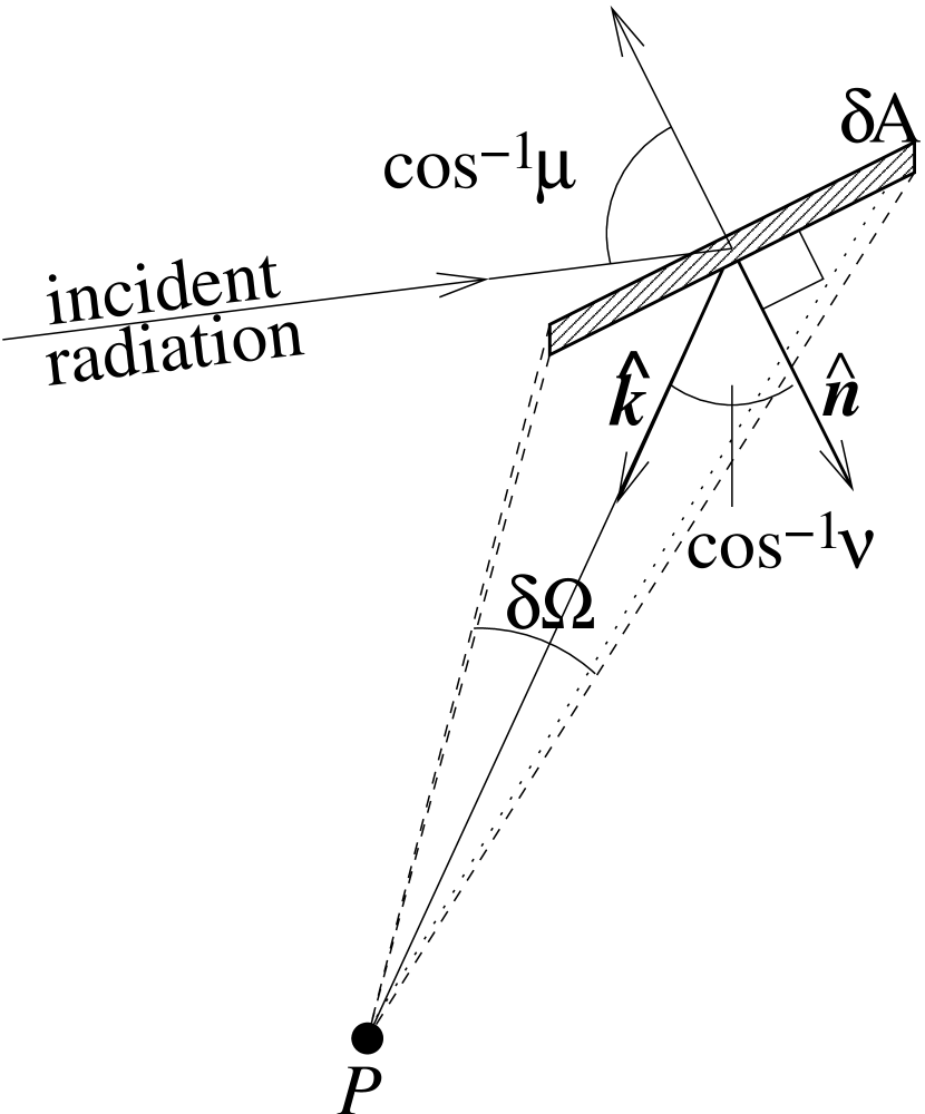
Figure 3: Angles involved in calculation of perturbed surface. See text for details.

Now we consider radiative transfer on a perturbed disk. A point $P(x,y,z)$ within the disk “sees” radiative flux coming from the surface of the disk. Each area element $\delta A$ contributes a solid angle $\delta\Omega$ of flux to $P$. Figure 3 shows a schematic of such an area element. The angle of incidence of radiation on this surface element is $\cos^{-1}\mu$. If $\mathbf{k}$ is the vector from $\delta A$ to $P$ and $\mathbf{\hat{n}}$ is the unit normal to $\delta A$, then $\nu$ is the cos of the angle between $\mathbf{\hat{n}}$ and $\mathbf{k}$.

We approximate the flux contribution from $\delta A$ as if it were a surface emitting isotropically with intensity

$$I=\frac{F_{d}(\tau_{d},\mu)}{\pi}.$$

and the corresponding contribution to the total flux is $d\mathbf{F}=I\,\mathbf{\hat{k}}\;d\Omega.$ Then the total flux at $P$ over all surface contributions is

$$\mathbf{F}_{\mathrm{tot}}=\frac{1}{\pi}\int F_{d}\,\mathbf{\hat{k}}\;\delta\Omega.$$ (20)

Since $\nabla$ is a linear operator,

$$\frac{1}{\kappa_{d}\rho}\nabla\cdot\mathbf{F}_{\mathrm{tot}}=\frac{1}{\pi}\int\frac{dF_{d}}{d\tau_{d}}\,\mathbf{\hat{n}}\cdot\mathbf{\hat{k}}\;\delta\Omega=4\pi\left(\frac{1}{\pi}\int J_{d}\,\nu\;\delta\Omega-\frac{1}{\pi}\int B\,\nu\;\delta\Omega\right).$$ (21)

Defining

$$J_{\mathrm{tot}} = \frac{1}{\pi}\int J_{d}(\tau_{d},\mu)\,\nu\;\delta\Omega\quad\mbox{and}$$ (22)

$$B_{\mathrm{tot}} = \frac{1}{\pi}\int B(\tau_{d},\mu)\,\nu\;\delta\Omega$$ (23)

we see that $\mathbf{F}_{\mathrm{tot}}$, $J_{\mathrm{tot}}$, and $B_{\mathrm{tot}}$ satisfy equations (8) and (9), and we can calculate the perturbed temperature as

$$T_{r}=\left(\frac{\pi B_{\mathrm{tot}}}{\sigma_{B}}\right)^{1/4}.$$ (24)

For a plane-parallel surface, $\tau_{d}$ and $\mu$ are constant, and $\nu=\cos\theta$, where $\theta$ is the angle with respect to the surface normal. We then recover the solution for the plane-parallel case.

This method of calculating radiative transfer can be applied to any three-dimensional disk configuration, including perturbations induced by protoplanets. Sufficiently massive protoplanets will open a gap in the disk, in which case the effects of shadowing and illumination across the gap can be calculated for all azimuthal angles. In the following section, we will calculate radiative transfer on small perturbations induced by planets too small to open a gap, but large enough to act on the disk locally.

3 Hydrostatic Equilibrium

Now we consider a perturbation induced by the gravitational potential of a protoplanet on a circumstellar disk. We shall consider only the gravitational effects of the protoplanet on hydrostatic equilibrium and assume that any resonant effects are washed out by gas drag.

3.1 Vertical Density Profile

In order to find the vertical structure of a non-self-gravitating gaseous disk orbiting a central star, we solve the equation of hydrostatic equilibrium:

$$\nabla P=-\rho\nabla\Phi$$ (25)

where $P$ is the gas pressure of the disk and $\Phi$ is the gravitational potential of the central star. Since we are interested in the vertical structure, we consider only the $z$ components and assume that the disk is isothermal in the $z$ direction. For a disk without a perturbing protoplanet, $\Phi=GM_{\star}/a$ where $M_{\star}$ and $a$ are the mass and distance of the star, respectively. If $c_{s}$ is the isothermal sound speed, then

$$c_{s}^{2}\,\frac{d\,\ln\rho}{dz}=-\frac{GM_{\star}}{a^{3}}z.$$ (26)

If we assume that $a\gg z$ and define $h\equiv c_{s}\,a^{3/2}/(GM_{\star})^{1/2}=(c_{s}/v_{\phi})a,$ then

$$\rho(z)=\rho_{0}\exp\left(-\frac{z^{2}}{2h^{2}}\right),$$ (27)

i.e. the density has a Gaussian distribution with a scale height of $h$ which is determined by the local temperature.

The insertion of a planet into a passive disk adds an additional term to $\Phi$, representing the potential due to the planet:

$$\Phi=GM_{\star}/a+Gm_{p}/r_{p}$$

where $m_{p}$ and $r_{p}$ are the mass and distance of the planet. Assuming that the planet is in the midplane ($z=0$), Eq. (26) becomes

$$\frac{d\,\ln\rho}{dz}=-\frac{z}{h^{2}}-\left(\frac{M_{p}a^{3}}{M_{\star}h^{2}}\right)\frac{z}{r_{p}^{3}}.$$ (28)

The Hill radius is defined as $r_{\mathrm{H}}\equiv(M_{p}/3M_{\star})^{1/3}a,$ and this equation integrates to

$$\rho(z)=\rho_{1}\exp\left[-\frac{z^{2}}{2h^{2}}+\frac{3r_{\mathrm{H}}^{3}}{h^{2}\,r_{p}}\right]$$ (29)

where $r_{p}=\sqrt{x^{2}+y^{2}+z^{2}}$, with the planet as the coordinate origin. So long as $r_{\mathrm{H}}\ll h$ and $|z|>r_{\mathrm{H}}$, the effect of the planet is a small perturbation on the density profile.

We normalize this equation by matching the density at $z=0$ to the unperturbed density, thus

$$\rho_{p}(z)=\rho_{0}\exp\left[-\frac{z^{2}}{2h^{2}}+\frac{3r_{\mathrm{H}}^{2}}{h^{2}}\left(\frac{r_{\mathrm{H}}}{\sqrt{x^{2}+y^{2}+z^{2}}}-\frac{r_{\mathrm{H}}}{\sqrt{x^{2}+y^{2}}}\right)\right]$$ (30)

Note that there is a singularity ar $r_{p}=0$. Figure 4 shows the shape of this density profile. In Figure 4a, we hold $r_{\mathrm{H}}/h$ fixed at $0.5$ and vary $\sqrt{x^{2}+y^{2}}$. For a disk with $h=0.04\>\mathrm{AU}$ at $1\>\mathrm{AU}$ around a central star of $0.5\>\mathrm{M}_{\sun}$, this corresponds to a protoplanetary mass of $4\>\mathrm{M}_{\oplus}$. For $(x^{2}+y^{2})\gtrsim r_{\mathrm{H}}^{2}$, the perturbed density profile does not deviate significantly from the unperturbed density profile. For $(x^{2}+y^{2})\lesssim r_{\mathrm{H}}^{2}$, the density profile develops a sharper profile at $z<h$. In Figure 4b, we hold $\sqrt{x^{2}+y^{2}}$ fixed at the Hill radius and vary the mass of the protoplanet, effectively varying $r_{\mathrm{H}}$. Larger protoplanets have the effect of decreasing the overall density profile, whereas position controls the shape of the profile, particularly close to the protoplanet. Since the flow of gas within the Roche lobe cannot be adequately described hydrostatically, we exclude the region $\sqrt{x^{2}+y^{2}}\lesssim r_{\mathrm{H}}$ from our analysis.

The normalization on equation (30) is somewhat arbitrary, but at the disk heights that are of interest to us, the overall normalization has small effect. We demonstrate this as follows: as $z\gg r_{\mathrm{H}}$, equation (30) becomes

$$\rho_{p}(z\gg r_{\mathrm{H}})\approx\rho_{0}\exp\left(-\frac{z^{2}}{2h^{2}}-\frac{3r_{\mathrm{H}}^{3}}{h^{2}\sqrt{x^{2}+y^{2}}}\right),$$ (31)

that is, a Gaussian with respect to $z$ with some normalization that depends on $r_{\mathrm{H}}$ and $\sqrt{x^{2}+y^{2}}$. The height of the photosphere, $H$, is generally several times the pressure scale height. If we take $H/h=5$, then the change in density with vertical distance is

$$\frac{\Delta\rho}{\rho}=\left|\frac{\Delta z}{\rho}\frac{d\rho}{dz}(z=H)\right|=\frac{25\Delta z}{H}.$$ (32)

So, a density change by a factor of $1/2$ corresponds to a shift in vertical height of 2%. In other words, the density gradient in the photosphere is so high that changes in the normalization of the density will not significantly affect our results.

3.2 Photosphere Height

We calculate the height of the perturbed photosphere from the perturbed density profile as the isodensity contour at the density of the unperturbed photosphere. That is, if $H_{0}$ is the unperturbed photosphere height and $H=H_{0}(1-\epsilon)$ is the new photosphere height, then we set

$$\rho_{d}(H_{0})=\rho_{p}(H)$$

or

$$-\frac{H_{0}^{2}}{2}=-\frac{H^{2}}{2}+3r_{\mathrm{H}}^{3}\left(\frac{1}{\sqrt{x^{2}+y^{2}+H^{2}}}-\frac{1}{\sqrt{x^{2}+y^{2}}}\right).$$ (33)

Setting $\sqrt{x^{2}+y^{2}}=\gamma H_{0}$, then to first order in $\epsilon$

$$H\approx H_{0}\left\{1-3\left(\frac{r_{\mathrm{H}}}{H_{0}}\right)^{3}\left[\frac{1}{\gamma}-\frac{1}{\sqrt{\gamma^{2}+1}}\right]\right\}$$ (34)

so that the depth of the perturbation scales as $(r_{\mathrm{H}}/H_{0})^{3}$. For typical disk models, the ratio of the photosphere height to the thermal scale height, $H_{0}/h$, is between 3 and 5, depending on the distance from the star and is often taken to be a constant (Kenyon & Hartmann, 1987; Chiang & Goldreich, 1997; D’Alessio et al., 1998). Restating the scaling of the depth of the perturbation as $\propto(r_{\mathrm{H}}/h)^{3}$, we see that this agrees with the estimate made in Sasselov & Lecar (2000).

The shape of this perturbed photosphere is shown in Figure 5 for varying values of $r_{\mathrm{H}}$. The perturbation is small for $r>r_{\mathrm{H}}$, and there is a singularity at $r=0$. As the Hill radius increases, the depth of the perturbation also increases. Note that if $H_{0}/h=5$, then $r_{\mathrm{H}}/H_{0}=0.2$ means that the Hill radius is comparable to the disk pressure scale height and the perturbation is no longer small. Protoplanets this massive are likely to open a gap in the disk rather than simply inducing a perturbation to the photosphere.

4 Disk Shear

The differential rotation of the disk causes the disk material near the protoplanet to move through the perturbation at a rate that depends on the velocity with respect to the protoplanet’s orbit. Material moving along a given streamline in the disk may pass through the perturbation too quickly to experience significant heating and cooling, thereby diminishing the effect of the perturbation on the temperature structure of the disk.

The velocity of the disk material with respect to the protoplanet is $v\simeq a(\Omega-\Omega_{p})$ where $\Omega$ and $\Omega_{p}$ are the orbital angular velocities of the disk material and the protoplanet, respectively, and $a$ is the orbital radius of the protoplanet. The orbital angular velocity of a gaseous disk is

$$r^{2}\Omega^{2}=\frac{GM_{\star}}{r}+\frac{1}{\rho}\frac{dP}{dr}.$$ (35)

In thin disks, such as we are investigating, the pressure gradient term is small so the orbital velocity is nearly equal to the Keplerian velocity.

The heating/cooling rate of the disk material can be expressed as

$$C\frac{\partial T}{\partial t}=F-\sigma T^{4}$$ (36)

where we take $F=\sigma(T_{v}^{4}+T_{r}^{4})$ and $C$ is the specific heat per unit surface area of the disk. We shall adopt a specific heat of $C=k\Sigma/m$ where $k$ is the Boltzmann constant, $\Sigma$ is the total surface density, and $m$ is the mean molecular mass.

We shall assume that the streamlines of the disk material follow equation (35), and that they are not perturbed by the protoplanet’s graviational potential. This is an adequate approximation for disk material outside the protoplanet’s Hill radius. Along each streamline, we calculate the total radiative flux, $F$, at a given position, and using the velocity of the streamline with respect to the protoplanet along with heating/cooling rate, we can calculate the steady state temperature at each position in the disk.

5 Model Parameters

Dust properties can be parametrized by $\alpha$, $\kappa_{s}$, and $q$. Then, the temperature profile in a plane-parallel disk is determined completely by $F_{v}$, $E_{0}$, $\mu_{0}$, and $\tau_{d}$, where $\tau_{d}$ is measured normal to the surface of the photosphere. Stellar properties determine $F_{v}$ and $E_{0}$, and the disk profile determines $\mu_{0}$. If $H_{0}\propto r^{\xi}$, then the incident angle is determined by

$$\mu_{0}=\frac{(\xi-1)H_{0}/a}{[1+(H_{0}/a)^{2}][1+\xi^{2}(H_{0}/a)^{2}]}$$ (37)

A perturbation changes the local angle of incidence and optical depth. In particular, without plane parallel symmetry, there is no single optical depth that parametrizes the distance below the surface. Instead, we sum over different lines of sight, using the optical depth along each line of sight to determine the contribution to the disk flux as in equation (23). The local angle of incidence depends only on the geometry of the perturbed surface, while the optical depth also depends on the density structure along the line of sight. The shape of the perturbed surface depends on $r_{\mathrm{H}}$ and $H_{0}$, and the density structure depends on the disk pressure scale height, $h$.

5.1 Fiducial Model

Motivated by observations of T Tauri stars, we will assume for our fiducial model that the central star has mass $M_{\star}=0.5\;\mathrm{M}_{\sun}$, radius $R_{\star}=2R_{\odot}$, and effective temperature $T_{\star}=4000$ K, and that the protoplanet is at $a=1\>\mathrm{AU}$ from the star. We assume an accretion rate of $\dot{M}_{a}=10^{-8}\;\mathrm{M}_{\sun}\,\mbox{yr}^{-1}$, so that $T_{v}=72$ K at $\tau_{d}=2/3$ at 1 AU. With these parameters, heating in the photosphere will be dominated by stellar irradiation rather than viscous heating. Near the midplane, however, viscous heating will dominate. Since we only consider the photosphere in our model, the calculation of the midplane temperature is outside the scope of this paper.

We will assume that the fraction of scattered radiation is $\alpha=0.28$, with opacity in the optical of $\kappa_{s}=400\;\mbox{cm}^{2}\mbox{g}^{-1}$, and ratio of opacities $q=20$.

We shall assume that $H_{0}=0.16\>\mathrm{AU}(r/1\>\mathrm{AU})^{9/7}$, consistent with e.g. D’Alessio et al. (1999a). In calculating the detailed density structure in the photosphere, we shall assume that $h=3.4\times 10^{-2}\>\mathrm{AU}$ so that $H_{0}/h=5$. A protoplanet with mass $m_{p}=1\;\mathrm{M}_{\oplus}$ ($10\>\mathrm{M}_{\oplus}$) will have a Hill radius of $1.26\times 10^{-2}\>\mathrm{AU}$ ($2.72\times 10^{-2}\>\mathrm{AU}$). As shown by Bate et al. (2003), planets with masses $\lesssim 30\>\mathrm{M}_{\oplus}$ are not massive enough to open a gap, and our perturbative treatment is valid. We have calculated models with $\>1\mathrm{M}_{\oplus}$, $10\>\mathrm{M}_{\oplus}$, and $20\>\mathrm{M}_{\oplus}$ planets, and present the results below.

5.2 Numerical details

We define our coordinate axes so that $x$ is aligned with the radial direction, $y$ is aligned with $\phi$ (i.e. the direction of planet’s orbit), and $z$ is perpendicular to the orbital plane. The coordinate origin is set at the surface of the disk above the planet position, so that the planet’s coordinates are $(0,0,-H_{0})$.

We calculate the shape of the disk surface in the $x$ and $y$ directions over a range $-10r_{\mathrm{H}}\leq x<10r_{\mathrm{H}}$ and $-10r_{\mathrm{H}}\leq y<10r_{\mathrm{H}}$, and use this surface to numerically integrate temperatures within the photosphere, to a depth of $z(\tau_{d}=2/3)=-0.011\>\mathrm{AU}$. The temperature is calculated at each point within a $64\times 64\times 64$ grid.

When summing over surface elements to find $B_{\mathrm{tot}}$ as in equation (23), we can approximate $\delta\Omega\approx\nu\delta A/\ell^{2}$ for $\delta A\ll\ell^{2}$, where $\ell$ is the distance between the point $P$ and $\delta A$. However, for points close to the surface, this approximation breaks down. In addition, $\nu$ may have large excursions over $\delta A$. For this reason, we assume that each $\delta A$ is approximately planar, so that $B(\tau_{d},\mu)$ does not vary, but we calculate $\int_{\delta\Omega}\nu\>d\Omega$ analytically from the limits of $\delta A$. In other words, we calculate

$$B_{\mathrm{tot}}=\frac{1}{\pi}\sum B(\tau_{d},\mu)\int\limits_{\delta\Omega}\nu\>d\Omega$$ (38)

and solve for the temperature.

6 Results

Figures 6, 7, and 8 show the spatial distribution of temperatures in the photosphere of the fiducial model for $1\>\mathrm{M}_{\oplus}$ $10\>\mathrm{M}_{\oplus}$, and $20\>\mathrm{M}_{\oplus}$ planets, respectively. The colors represent temperatures in Kelvin, as indicated by the colorbars. The horizontal axis indicates increasing radial distance from the star so that the photosphere is illuminated from the left. The cross-section is taken at the $\tau_{d}=2/3$ surface. The bottommost row and leftmost column show the unperturbed temperature of $133.6\>\mathrm{K}$ for comparison. This temperature is also indicated in the colorbar by a dotted white line.

The direction of the planet’s orbit is upward on the plots, so the interior disk material moves faster, and the exterior disk material moves slower than the planet. This causes the heated and cooled regions to shear out. The positions of minimum and maximum temperatures are offset from the planet’s position since it takes some time for the heated/cooled material to come back to the equilibrium temperature.

For a $1\>\mathrm{M}_{\oplus}$ protoplanet, the shadowing and illumination at the surface results in a slight temperature change, with the area to the right of the planet reaching a maximum temperature of $135.5\>\mathrm{K}$, and the area to the left cooled to a minimun of $130.7\>\mathrm{K}$ – a change of $-2.2\%$ to $+1.4\%$. Thus, we see that an Earth-mass planet is too small significantly affect the interior temperature of the disk.

A larger planet will create a larger perturbation, which will lead to a greater temperature change. Figure 7 and Figure 8 show the temperature distribution in the photosphere for a $10\>\mathrm{M}_{\oplus}$ planet and $20\>\mathrm{M}_{\oplus}$ planet, respectively. The plots are scaled to the Hill radius, which goes as $m_{p}^{1/3}$, so the physical range in Figures 7 and 8 is actually larger than that in Figure 6. The high temperatures close to the Hill radius are due to the low density in this region, which gives a low optical depth to the illuminated surface. However, since this region is not in hydrostatic equilibrium, we exclude it from our analysis. Outside the Hill radius, the temperatures at $\tau_{d}=2/3$ for a $10\>\mathrm{M}_{\oplus}$ protoplanet range from $123.7\>\mathrm{K}$ to $142.3\>\mathrm{K}$, or by $-7.4\%$ to $+6.5\%$. For a $20\>\mathrm{M}_{\oplus}$ protoplanet, which is close to but not at the limit where a gap in the disk can form, the temperature range increase slightly, with a minimum of $122.0\>\mathrm{K}$ and maximum of $146.6\>\mathrm{K}$, or by $-9.7\%$ to $+8.7\%$. Thus, a protoplanet with mass 10 $\mathrm{M}_{\oplus}$ or larger may have a significant effect on the local temperature structure of a protoplanetary disk.

7 Discussion

As planet-forming disks are likely to be passive (Calvet et al., 2002), we have explored stellar irradiation effects due to a disk surface perturbation induced by an embedded protoplanet. We find that even a relatively small protoplanet (in the range from 1 to 20 Earth mass) produces enough of a perturbation to cause shadowing. In particular, we find that in a standard passive disk accreting at $10^{-8}\>\mathrm{M}_{\sun}\mathrm{yr}^{-1}$, the temperature variation induced by a $1\>\mathrm{M}_{\oplus}$ planet at 1 AU is $5\>\mathrm{K}$, or only about $4\%$. However, we find that even though a protoplanet may not be massive enough to open a gap in a disk, it may still be able to significantly change the temperature structure in a the disk material near it. A $10\>\mathrm{M}_{\oplus}$ ($20\>\mathrm{M}_{\oplus}$) planet can induce a temperature variation of $19\>\mathrm{K}$ ($25\>\mathrm{K}$), or $14\%$ ($18\%$).

This results in a local temperature perturbation which is large enough to affect the local properties of the disk and the accretion rate, and possibly the migration rate of the protoplanet. Although the perturbation in temperature may be too subtle to directly observe, it can have serious consequences for planet growth and migration.

Ward (1997) has shown that the rate of Type I migration is strongly dependent upon the temperature gradient of the disk. If the temperature decreases with distance from the star, then the total net torques result in inward migration of the secondary. However, if $k=-d\ln T/d\ln r\lesssim-1$, then the opposite is true and the secondary will migrate outward. The temperature perturbation near a protoplanet locally decreases the value of $k$, and may result in halting or even reversing Type I migration. This may resolve the conundrum that Type I migration timescales are typically much less than observed disk lifetimes of $\sim 10^{7}$ years (Hartmann et al., 1998). Yet to date, no simulation of planet-disk interactions accounts for local temperature pertubations as described here.

We have not yet considered the behavior of the dust (as a function of size) in the perturbed region. We expect the dust to remain coupled to the gas and compress its scale height accordingly. In fact crude estimates of dust sedimentation in the vicinity of the planet confirm that. However, a detailed estimate of the sedimentation timescale is necessary in order to evaluate the amount of residual dust, e.g. swept by stellar radiation from the inner edge, and its total opacity. These are issues we plan to address in future work.

In a forthcoming paper, we will undertake a parameter study of our model for radiative transfer on a perturbed disk. By varying attributes of the disk, star, and protoplanet, we will investigate the possibility that a relatively small protoplanet which is not large enough to open a gap in a disk might still be able to affect disk structure.

Figure 1: Schematic of a flared disk. Proportions are not to scale. The labels thick and thin refer to optical depth in short and long wavelengths.

Figure 2: The temperature due solely to stellar irradiation at the surface of the disk (dashed line) and in the interior (solid line) for varying values of the angle of incidence, $\mu_{0}$, where $T_{0}=(E_{0}/\sigma_{B})^{1/4}$.

Figure 4: Perturbed vertical density profile for varying parameters. Density is normalized to the midplane density. Both plots are to the same scale and show the unperturbed density profile as a solid line. (a) Density profile for fixed Hill radius and varying values of $(x^{2}+y^{2})^{1/2}$ as indicated. (b) Density profile for $(x^{2}+y^{2})^{1/2}$ equal to the Hill radius and varying planetary masses.

Figure 5: Perturbed photosphere height as a function of distance in the $xy$-plane, $r$, for varying Hill radii. The solid vertical line indicates where $r=r_{\mathrm{H}}$.

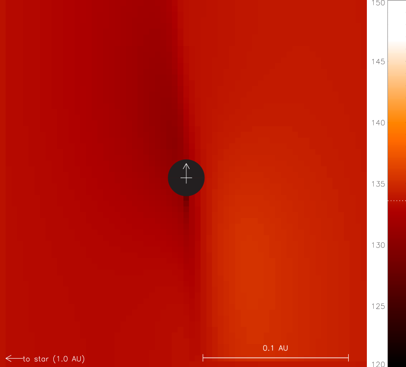
Figure 6: Temperature profile of the disk photosphere near a protoplanet of mass 1 $\mathrm{M}_{\oplus}$ at $\tau_{d}=2/3$ in the $xy$-plane. The colors indicate the temperature in Kelvin, scaled as shown in the colorbar. The cross in the center represents planet position, with the arrow indicating the direction of the planet’s orbit. The blacked-out circle indicates the extent of the Hill radius. The dotted white line in the color bar indicates the unperturbed temperature at $\tau_{d}=2/3$.

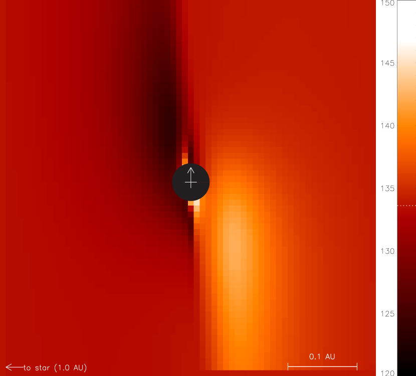
Figure 7: Same as Figure 6, for a protoplanet of mass 10 $\mathrm{M}_{\oplus}$. Note that the dimensions on the figures scale with the Hill radius, so the physical sizes of the plots are $10^{1/3}$ larger than in Figure 6.

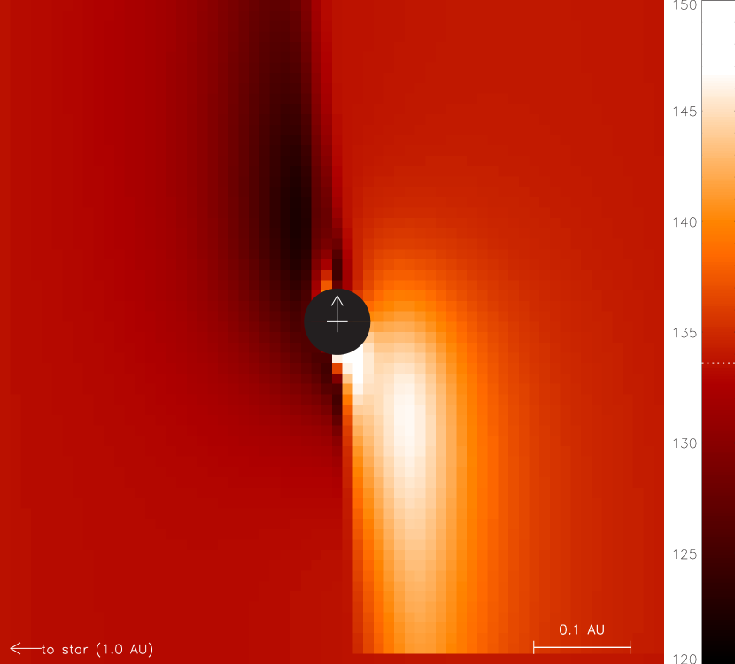
Figure 8: Same as Figure 6, for a protoplanet of mass 20 $\mathrm{M}_{\oplus}$.

References

- Bate et al. (2003) Bate, M. R., Lubow, S. H., Ogilvie, G. I., & Miller, K. A. 2003, MNRAS, submitted (astro-ph/0301154)
- Calvet et al. (2002) Calvet, N., D’Alessio, P., Hartmann, L., Wilner, D., Walsh, A., & Sitko, M. 2002, ApJ, 568, 1008
- Calvet et al. (1991) Calvet, N., Patino, A., Magris, G. C., & D’Alessio, P. 1991, ApJ, 380, 617
- Chiang & Goldreich (1997) Chiang, E. I. & Goldreich, P. 1997, ApJ, 490, 368
- D’Alessio et al. (1999a) D’Alessio, P., Calvet, N., Hartmann, L., Lizano, S., & Cantó, J. 1999a, ApJ, 527, 893
- D’Alessio et al. (1999b) D’Alessio, P., Cantó, J., Hartmann, L., Calvet, N., & Lizano, S. 1999b, ApJ, 511, 896
- D’Alessio et al. (1998) D’Alessio, P., Canto, J., Calvet, N., & Lizano, S. 1998, ApJ, 500, 411
- Hartmann et al. (1998) Hartmann, L., Calvet, N., Gullbring, E., & D’Alessio, P. 1998, ApJ, 495, 385
- Kenyon & Hartmann (1987) Kenyon, S. J. & Hartmann, L. 1987, ApJ, 323, 714
- Milne (1930) Milne, E. A. 1930, Handbuch der Astrophysik, 3, 65
- Pringle (1981) Pringle, J. E. 1981, ARA&A, 19, 137
- Sasselov & Lecar (2000) Sasselov, D. D. & Lecar, M. 2000, ApJ, 528, 995
- Strittmatter (1974) Strittmatter, P. A. 1974, A&A, 32, 7
- Ward (1997) Ward, W. R. 1997, Icarus, 126, 261