Optimal Moments for the Analysis of Peculiar Velocity Surveys II: Testing

Abstract

Analyses of peculiar velocity surveys face several challenges, including low signal–to–noise in individual velocity measurements and the presence of small–scale, nonlinear flows. This is the second in a series of papers in which we describe a new method of overcoming these problems by using data compression as a filter with which to separate large–scale, linear flows from small–scale noise that can bias results. We demonstrate the effectiveness of our method using realistic catalogs of galaxy velocities drawn from N–body simulations. Our tests show that a likelihood analysis of simulated catalogs that uses all of the information contained in the peculiar velocities results in a bias in the estimation of the power spectrum shape parameter $\Gamma$ and amplitude $\beta$, and that our method of analysis effectively removes this bias. We expect that this new method will cause peculiar velocity surveys to re–emerge as a useful tool to determine cosmological parameters.

Subject headings: cosmology: distance scales – cosmology: large scale structure of the universe – cosmology: observation – cosmology: theory – galaxies: kinematics and dynamics – galaxies: statistics

1 INTRODUCTION

Although in principle the measurement of galaxy motions holds great promise as a probe of large–scale structure, in practice there are several obstacles that have prevented there from being robust conclusions made from the analyses of these measurements. First, these measurements are inherently noisy; errors in peculiar velocity determinations are typically of order $10\%$ of the redshift of a galaxy or cluster, which for all but nearby objects is comparable or larger than the velocity being measured. From the theoretical side, in order to relate the velocity field to the underlying matter density one must assume that the fields are linear. While this approximation is accurate on large scales, on smaller scales it generally fails due to infall into density concentrations. The difficulty in surmounting these obstacles is illustrated in the fact that attempts to compare different velocity field surveys have shown significant disagreements (Watkins & Feldman,, 1995; Hudson et al. , 1999).

Analyses of catalogs of peculiar velocity measurements have usually taken either of two main approaches. One is to average all the velocities to find the bulk flow, the velocity of the volume occupied by the survey relative to the Universal rest frame defined by the CMBR (e.g. Lauer & Postman (1994); Riess, Press & Kirshner (1995); Branchini, Plionis & Sciama (1996); Colless etal (2001); Aghanim & G rski (2001)). This method has the disadvantage that it discards most of the information contained in a survey and measures only three quantities, the components of the bulk flow vector. The second approach is to use all of the information contained in the survey in a likelihood analysis in order to obtain maximum likelihood estimates of the power spectrum parameters (e.g. Zaroubi et al.  (2001); Yang et al.  (2001); Zehavi & Dekel (2000); Freudling et al.  (1999)). This method potentially suffers from a bias due to small–scale, nonlinear contributions to velocities.

In a recent paper (Watkins et al.  (2002), hereafter Paper I), we introduced a new method for the analysis of peculiar velocity surveys that is a significant improvement over previous methods. In particular, our formalism allows us to separate information about large–scale flows from information about small scales, the latter which can then be discarded in the analysis. By applying specific criteria, we are able to retain the maximum information about large scales needed to place the strongest constraints, while removing the bias that small scale information can introduce into the results.

In paper I we reported on preliminary tests that suggested that our analysis method was effective. Here we present results from more extensive testing that demonstrates conclusively that our method works as advertised. In particular, we show that a likelihood analysis of simulated catalogs that uses all of the information contained in the peculiar velocities results in a bias in the estimation of the power spectrum parameters $\Gamma$ and $\beta$, and that our method of analysis effectively removes this bias.

The paper is organized as followed: in sections 2 and 3 we briefly review the analysis formalism introduced in Paper I. In section 4 we discuss the N–body simulations we used and how we constructed synthetic catalogs. In section 5 we discuss results from our synthetic catalogs for both a full likelihood analysis of the catalog as well as our new analysis method. We also present additional evidence that our method is working effectively. In section 6 we conclude.

2 The Formalism

Our starting point is the usual statistical model for the line–of–sight peculiar velocities of galaxies. First, we assume that galaxies are tracers of a large–scale linear velocity field ${\bf v(\bf x)}$, a Gaussian random field completely described by the velocity power spectrum $P_{(v)}(k)$. With the assumption of linearity, the velocity power spectrum is proportional to the power spectrum of density fluctuations, with $P_{(v)}(k)=H_{o}^{2}\Omega^{1.2}P(k)$.

For a set of $N$ galaxies with positions ${\bf r_{i}}$, the observed line–of–sight velocity will be given by

$$v_{i}={\bf v}({\bf r}_{i})\cdot{\bf\hat{r}}_{i}+\delta_{i},$$ (1)

the sum of the radial component of the velocity field with a noise term $\delta_{i}$ describing both observational error and any deviation from the linear velocity field due to local gravitational interactions. For simplicity we assume that $\delta_{i}$ is distributed as a Gaussian random variable with variance $\sigma_{i}^{2}+\sigma_{*}^{2}$, where $\sigma_{i}$ is the observational error associated with that particular galaxy, and $\sigma_{*}$ describes all other effects and is assumed to be the same for all the galaxies in the set.

With these assumptions, we can construct the probability distribution for the set of measured line–of–sight velocities given a power spectrum $P(k)$,

$$L(v_{1},...,v_{N};P(k))=\sqrt{|R^{-1}|}\ \exp\left(\sum_{i,j=1}^{N}-v_{i}R^{-1}_{ij}v_{j}/2\right),$$ (2)

where $R_{ij}=\langle v_{i}\ v_{j}\rangle$ is the covariance matrix, which in this case takes the form

$$R_{ij}=R^{(v)}_{ij}+\delta_{ij}\,(\sigma_{i}^{2}+\sigma_{*}^{2})$$ (3)

where $R^{(v)}_{ij}=\langle{\bf v}({\bf r}_{i})\cdot{\bf\hat{r}}_{i}\ \ {\bf v}({\bf r}_{j})\cdot{\bf\hat{r}}_{j}\rangle$ and the second diagonal term is due to the noise. In linear theory, the “signal” part of the covariance matrix $R^{(v)}$ can be written as an integral over the density power spectrum

$$R^{(v)}_{ij}={H^{2}\Omega_{o}^{1.2}\over 2\pi^{2}}\int P(k)W^{2}_{ij}(k)\ dk,$$ (4)

where $W^{2}_{ij}(k)$ is a tensor window function calculated from the set of positions ${\bf r}_{i}$ of the galaxies with galaxy velocities weighted by their relative error (for more details see Feldman & Watkins (1994); Watkins & Feldman, (1995); Feldman & Watkins (1998)).

Typically we are given the a catalog of measured velocities $(v_{1},...,v_{N})$ and wish to determine $P(k)$. Thus we can view $L(v_{1},...,v_{N};P(k))$ as a likelihood functional; given $(v_{1},...,v_{N})$ we use Eq. (2) to determine the likelihood that they were generated in a Universe with a particular $P(k)$.

An analysis of the type described above is susceptible to biases due to small–scale, nonlinear contributions to the galaxy velocities. The method of analysis developed in Paper I eliminates this bias by replacing the full set of $N$ line–of–sight velocities $v_{i}$ with moments $u_{i}$, which are designed so that the $N$th moment is the linear combination that carries the most information about small scales, the $(N-1)$th moment is an independent linear combination which carries the second most small–scale information, etc. By using a subset of the first $N^{\prime}<N$ moments in our analysis and discarding the rest, we can essentially filter out the small scale information which may carry nonlinear contributions. Our method is based on Karhunen–Loève methods of data compression (Kenney & Keeping, 1954; Kendall & Stuart, 1969); see also Tegmark, Taylor & Heavens (1997), designed to concentrate most of the information in a large set of data into a smaller, more manageable number of moments. However, our method puts a twist on this idea by concentrating unwanted information regarding small scales into a small set of moments which can then be discarded. What follows is a brief review of the mechanics of our method; for details, see Paper I.

Our method is based on linear data compression, so that the moment $u_{n}$ can be written in terms of the line–of–sight velocities $v_{i}$ as

$$u_{n}=\sum_{j=1}^{N}(b_{n})_{j}\ v_{j}\ ,$$ (5)

where the $b_{n}$ are a set of vectors of length $N$. With this definition, the covariance matrix of the new moments is given as

$${\tilde{R}_{nm}}=\langle u_{n}u_{m}\rangle=\sum_{i,j}(b_{n})_{i}\langle v_{i}v_{j}\rangle(b_{m})_{j}=\sum_{i,j}(b_{n})_{i}R_{ij}(b_{m})_{j}\ .$$ (6)

It is convenient to choose the $b_{n}$ so that the $u_{n}$ are linearly independent and of unit variance, so that ${\tilde{R}_{nm}}$ is the identity matrix. Note that this normalization will hold only for a particular matrix $R_{ij}$ and hence a particular power spectrum.

In order to find the vector $b_{n}$ such that the moment $u_{n}$ carries the maximum information about nonlinear scales, we assume a simple model for the power spectrum in which the amount of power on scales below that where density fluctuations have gone nonlinear is specified by a single parameter $\theta_{q}$. Given a single moment $u_{n}$, we can determine the value of $\theta_{q}$ to within a minimum variance given by $\Delta\theta_{q}^{2}=1/{\tilde{F}}_{qq}$, where ${\tilde{F}}_{qq}$ is the $qq$th element of the Fisher information matrix, which in this case, and with the normalization assumed above, can be shown to take the form

$${\tilde{F}_{qq}}=\sum_{ij}{1\over 2}\left((b_{n})_{i}{\partial R_{ij}\over\partial\theta_{q}}(b_{n})_{j}\right)^{2}$$ (7)

We can thus find the single moment $u_{n}$ that carries the maximum information about $\theta_{q}$ by finding the vector $b_{n}$ which minimizes ${\tilde{F}}_{qq}$ subject to the normalization condition discussed above, which functions as a constraint. After introducing a Lagrange multiplier, the minimization results in an eigenvalue problem

$$\sum_{i,j,m}\left(L^{-1}_{ki}{\partial R_{ij}\over\partial\theta_{q}}L^{-1}_{lj}\right)\left(L_{ml}b_{m}\right)=\sum_{j}\lambda\left(L_{jk}b_{j}\right)$$ (8)

where $L_{ij}$ is the Cholesky decomposition of the covariance matrix, $R_{ij}=\sum_{p=1}^{N}L_{ip}L_{jp}$.

Solving this eigenvalue problem gives us a set of $N$ orthogonal eigenvectors $\sum_{j}L_{ji}(b_{n})_{j}$ with eigenvalues $\lambda_{n}$. Each eigenvector has a corresponding moment $u_{n}=\sum_{i}(b_{n})_{i}v_{i}$. The eigenvalue $\lambda_{n}$ of a moment $u_{n}$ is related to the error bar $\Delta\theta_{q}$ that one could place on $\theta_{q}$ using the single moment $u_{n}$, as can be seen by manipulating the equations above:

$${1\over\Delta\theta_{q}^{2}}={\tilde{F}}_{qq}=\sum_{i,j}{1\over 2}\ (b_{i}{\partial R_{ij}\over\partial\theta_{q}}b_{j})^{2}=\sum_{i,j}{1\over 2}\ ({b_{i}\left(\lambda R_{ij}b_{j}\right)})^{2}={\lambda^{2}\over 2}$$ (9)

so that $\Delta\theta_{q}=2/\lambda^{2}$. If we order the moments $u_{n}$ in order of increasing eigenvalue,

$$|\lambda_{1}|\leq|\lambda_{2}|\leq\ldots\leq|\lambda_{N}|$$ (10)

then we can interpret each moment as carrying successively more information about $\theta_{q}$, with $u_{N}$ carrying the maximum possible amount of information. Since our goal is to produce a data set that is less sensitive to the value of $\theta_{q}$ than the original data, we should keep moments only up to some $N^{\prime}$. The orthogonality of the eigenvectors ensures that the moments are statistically independent, as we assumed above. Thus if we compress the data by discarding the moments with a large value of $|\lambda|$, the information contained in those moments will be completely removed from the data. However, we would also like to keep as many moments as possible in order to retain the maximum information about large scales.

In order to choose a value of $N^{\prime}$, we need to examine what error bar $\Delta\theta_{q}$ we can put on the parameter $\theta_{q}$ using the compressed data. Since the moments are independent, we can write the Fisher matrix for the $N^{\prime}$ moments that were not discarded as

$$\tilde{F}_{qq}=\sum_{n=1}^{N^{\prime}}{1\over 2}\lambda_{n}^{2}$$ (11)

so that the error bar that can be put on $\theta_{q}$ using the compressed data is given by

$$\Delta\theta_{q}={1\over\sqrt{\tilde{F}_{qq}}}=\left[{1\over 2}\sum_{n=1}^{N^{\prime}}\ \lambda_{n}^{2}\right]^{-1/2}$$ (12)

This suggests that $N^{\prime}$ should be chosen by adding up the sum of the squares of the smallest eigenvalues until the desired sensitivity is reached. The criterion that we use is as follows: First, we estimate the actual size of the parameter $\theta_{q}=\theta_{qo}$ from peculiar velocity data. Then, we keep the largest number $N^{\prime}$ moments that is still consistent with the requirement that $\Delta\theta_{q}\geq\theta_{qo}$. With this requirement, as long as our estimate of the true value of $\theta_{q}$ is correct, our final set of moments $u_{1}\ldots u_{N^{\prime}}$ will not contain enough information to distinguish the value of $\theta_{q}$ from zero.

3 Other Selection Criteria

Our method of selecting moments by their lack of information about small scales has the disadvantage of not discarding moments which have little information about any scale; this issue was briefly touched on in Paper I. Thus we have developed a second criterion for moment selection whereby we discard moments that are dominated by noise. That is, they have no cosmologically useful information.

Recall from Eq. 3 that the covariance matrix for the line–of–sight velocities is the sum of a “signal” part and a noise part. Since the covariance matrix for the moments $u_{n}$ is essentially a “rotation” of the velocity covariance matrix, this matrix can separated in a similar fashion,

$$\tilde{R}_{nm} = \sum_{ij}(b_{n})_{i}R_{ij}(b_{m})_{j}=\sum_{ij}(b_{n})_{i}R^{(v)}_{ij}(b_{m})_{j}+\sum_{ij}(b_{n})_{i}\delta_{ij}(\sigma_{i}^{2}+\sigma_{*}^{2})(b_{m})_{j}$$ (13)

$$= \tilde{R}_{nm}^{(v)}+\sum_{i}(b_{n})_{i}(b_{m})_{i}(\sigma_{i}^{2}+\sigma_{*}^{2})$$

where the second term is the noise contribution to the variance of the moment. Given that the $b_{n}$ are normalized such that the moments are independent and have unit variance, i.e. that $\tilde{R}$ is the identity matrix, we see that the quantity

$$\xi_{n}=\sum_{i}(b_{n})_{i}^{2}(\sigma_{i}^{2}+\sigma_{*}^{2})$$ (14)

is a measure of the fraction of the variance of the moment $u_{n}$ that is due to noise. If $\xi_{n}\ll 1$, then the moment has very little noise and should be retained. If, on the other hand, $\xi_{n}\approx 1$, then the value of the moment is mostly determined by the errors in the data and should be discarded.

Generally there is a correlation between a moment’s $\xi_{n}$ and its eigenvalue $|\lambda_{n}|$; moments that are most sensitive to small scales tend to be very noisy. Low noise moments tend to be those that probe large–scale power. This is due to the fact that the measurement errors in the velocities, which vary independently from galaxy to galaxy, are much more effective at masking small scale modes than large scale modes. However, we have found that some moments with small eigenvalues also have large noise; these moments carry little information about any scale.

The correlation between $\xi_{n}$ and $|\lambda_{n}|$ suggests that our two selection criterion can be somewhat redundant; eliminating noisy moments often can also accomplish the goal of removing moments with large $|\lambda_{n}|$. Similarly, eliminating moments with large $|\lambda_{n}|$ leaves one with moments which generally have smaller noise. Thus we will see below that applying the second criteria after we have already applied the first typically does not change the results of the analysis significantly.

Once one has a set of moments which have both small $\xi_{n}$ and $|\lambda_{n}|$, it is desirable to have a way of determining which scales each moment is most sensitive to. From Eq. 4 we recall that the “signal” part of the covariance matrix for the velocities $R^{(v)}$ is given by an integral of a tensor window function $W_{ij}(k)$ with the power spectrum. The “signal” part of the covariance matrix $\tilde{R}$ of the moments is given by a “rotation” of this tensor window function. Since $\tilde{R}$ is diagonal, this results in a scalar window function for each moment $u_{n}$,

$$W^{2}_{n}(k)=(b_{n})_{i}W^{2}_{ij}(k)(b_{n})_{j}$$ (15)

By examining the window functions for each moment, we can determine which scales the moments are sensitive to and confirm that our method is working. In principle, examination of the window functions could also provide a further criterion for the discarding of moments.

4 Synthetic Catalogs

The simulations used here are numerical models for the gravitational dynamics of collisionless particles in an expanding background. We are studying evolution of initial Gaussian perturbations in a matter–dominated universe. All the simulations are done with a particle–mesh (PM) code with $256^{3}$ particles in an equal number of grid points (Melott, 1986; Melott, Weinberg & Gott, 1988). More details about the peculiarities of the simulations used here can be seen in Melott & Shandarin (1993). Although the parameter $\Omega$ appears in both the dynamics of the expanding background and as a parameter in the fit to the power spectrum shape in the CDM family of models (Bardeen et al. , 1986), they serve two different functions.

We ran simulations with a dynamical background $\Omega_{0}$ = 1. or 0.34. These were normalized to an amplitude $\sigma_{8}$=0.93 at redshift moment $z$=0, but we also took data at $z$=1, which for our purposes can be described as studying a Universe with a lower perturbation amplitude normalization, and possibly a higher $\Omega_{0}$. All models were interpreted with an assumed Hubble Constant H$=100h$km s^-1Mpc^-1 where $h$ = 2/3. When power spectra are parameterized in $Mpc$, the shape is dependent upon $\Omega_{0}h^{2}$, which we set equal to 0.15, 0.35, and 1.0 for our low–$\Omega$ tests. We have used some values which are inconsistent with other constraints in CDM linear theory in order to test our method over a wide range of values. We also ran another simulation with $\Omega_{0}$ = 1, and $\Omega_{0}h^{2}$ = 0.15; such models have been called $\tau$CDM in the past. The set with $\Omega_{0}$ = 0.34, $\Omega_{0}h^{2}$ = 0.15 is most consistent with a variety of findings at this time, but we do not wish to test our method only against currently favored cosmologies. There are a variety of alternative models in addition to the cosmological constant $\lambda$; all have very small and totally linear effects on large–scale velocities. We omit this in favor of wider exploration of parameter shifts which have large effects.

For testing our method we created synthetic redshift–distance catalogs from the 256³ $N$–body PM simulations. In these simulations, the box size was taken to equal 512 Mpc, or 34,133 km s^-1 in redshift space for $h$=2/3.

Each of the points defined by the mesh represented a galaxy with a corresponding location and velocity. Testing the optimal moments method accurately requires proper modeling of statistical errors so we wanted to be sure to include the effects of cosmic variance and scatter in distance indicators. We chose three coordinates of scale 1/6, 1/2 and 5/6 the box width. An exhaustive permutation of combining these coordinates results in 27 center locations within the box, each corresponding to an individual synthetic catalog as described next. About each central location, an annular volume was defined by the redshift range 500 km s${}^{-1}<$ z $<$ 10,000 km s^-1. If the volume intercepted the boundaries of the box then we appealed to the periodic boundary conditions of the simulation and included galaxies from the opposite box side. Within each of the defined regions, we selected $\approx$ 1000 galaxies under the assumption of a radial selection function and the additional requirement that there is a zone of avoidance below the galactic latitude $|b|<10^{\circ}$. The selection function was chosen generically (we ignored galactic properties) to mimic existing popular redshift–distance surveys (i.e. the SFI survey; da Costa et al. (1996)). The effect of scatter in distance indicators was replicated by adding a random error to each peculiar velocity drawn from a Gaussian distribution of width 10% of the galaxy redshift distance.

In the end, for each simulation box we have 27 surveys sampling the simulation that give information about the positions and radial velocities of the galaxy distribution in some volume. We analyzed these surveys by using the actual positions (i.e. no errors) and by perturbing the velocities with a 10% Gaussian error. The value of sampling the simulation in this way is that we are able to model the effects of cosmic variance. The errorbars of the unperturbed catalogs are predominantly from the cosmic variance, whereas those of the perturbed, 10% catalogs include the effects of both cosmic variance and the inaccuracies of the distance indicators.

5 Results

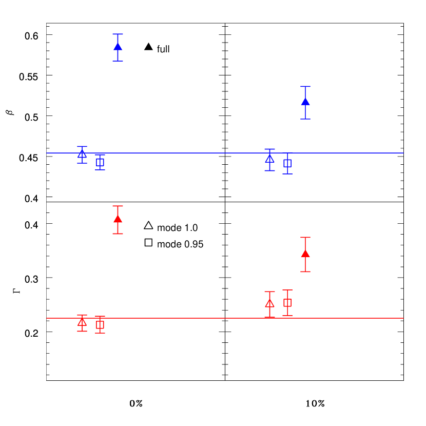
Figure 1: A comparison between the mode analysis presented in this paper and the traditional full analysis. The results are from 81 catalogs extracted from the simulations (see Sec. 4). In the top two panels are the mean values and standard deviations of the mean of $\beta$, the amplitude of the power spectrum. The bottom panels we show the results for estimating $\Gamma$, the shape parameter. In the left panels we have the results for the analysis for a survey with no errors whereas the right panels show the results for 10% errors. The solid symbols are the full analysis results and the empty ones are the mode analysis. The triangles are the results without removing the noisy moments, the rectangles are those where we removed the noisiest moments. The horizontal lines are the “true” values of the parameters ($\Gamma=0.225$, $\beta=0.455$). It is clear that the full analysis fails to recover the parameter values whereas the mode analysis recovers them well.

The main purpose of the formalism we presented here and in Paper I was to allow the removal or filtering of small scale noise while keeping the large scale signal. To test the success of the formalism we have created synthetic surveys from simulations with known parameters, specifically, $\Gamma$, the CDM power spectrum shape parameter, and $\beta$, its amplitude (the values of the parameters we simulated is given in the table 1 below.) To compare our method with the full analysis method, we reemphasize that the optimal moment analysis presented here allows for two semi–independent methods of cleaning up a survey: 1) Ordering the moments by their eigenvalues (Eq. 10); and 2) Removing the noisiest moments (Eq. 14). In Figs. 1 and 3–6 we show the comparison between choosing the modes least susceptible to small scale signal (open triangles); those that are least susceptible to small scale signal and are not noisy (open squares); and the full analysis (that is, keeping all moments, the usual analysis, solid triangles). We see that the full analysis fails to recover the “true” parameters by a significant amount ($\approx 4\sigma$ for no errors and $>2\sigma$ for 10% errors). In contrast, the mode analysis recovers the values of the parameters very well, with or without the removal of the noisy moments.

$\Gamma_{T}$	$\beta_{T}$	Analysis	$<\Gamma>$	$\sigma_{\Gamma}$	$<\beta>$	$\sigma_{\beta}$
0.225	0.455	mode	0.21 $\pm$ 0.016	0.14	0.44 $\pm$ 0.009	0.08
		full	0.41 $\pm$ 0.026	0.23	0.58 $\pm$ 0.017	0.15
0.225	0.372	mode	0.22 $\pm$ 0.014	0.11	0.38 $\pm$ 0.008	0.06
		full	0.28 $\pm$ 0.019	0.14	0.40 $\pm$ 0.010	0.07
0.510	0.410	mode	0.47 $\pm$ 0.066	0.35	0.41 $\pm$ 0.019	0.10
		full	0.90 $\pm$ 0.079	0.41	0.59 $\pm$ 0.031	0.16
0.510	0.330	mode	0.46 $\pm$ 0.051	0.26	0.34 $\pm$ 0.015	0.08
		full	0.68 $\pm$ 0.067	0.35	0.41 $\pm$ 0.019	0.10
0.667	0.320	mode	0.58 $\pm$ 0.068	0.35	0.31 $\pm$ 0.015	0.08
		full	0.94 $\pm$ 0.029	0.15	0.47 $\pm$ 0.016	0.08

Table 1: The values of the parameters for the simulations used to extract the catalogs we used to test our formalism. $\Gamma_{T}$ and $\beta_{T}$ are the “true” values of our parameters for each simulation. The Analysis column denotes our proposed formalism (mode) and the full maximum likelihood analysis (full). The $<\Gamma>$ and $<\beta>$ columns show the mean and the standard deviation of the mean of the parameters for each simulation. The $\sigma_{\Gamma}$ and $\sigma_{\beta}$ columns are the standard deviations for the parameters. When comparing the maximum likelihood values, the mode analysis does a much better job recovering to the “true” values then does the full analysis.

For each one of the models we simulated we have extracted 27 catalogs from each simulation box, as described in Sec. 4. The points and errorbars in the figures are the maximum likelihood mean and standard deviation of the mean for the analysis of all catalogs. Each one of the catalogs were analyzed using the full maximum likelihood analysis, keeping all moments; the maximum likelihood analysis discarding large eigenvalue modes; and the maximum likelihood mode analysis without the noisiest moments ($\xi>0.95$).

In Fig. 2 we show the value of the estimated parameters as a function of the $\Sigma\lambda^{2}$ (see Eq. 12) where we see that as the number of modes is increased, we get closer and closer to the “true” value. When we keep more than the number of moments that corresponds to the fulfillment of our criterion (Eq. 12), the values start diverging from the “true” results. This is due to the fact that small–scale modes that have become nonlinear are introducing a bias. This tendency of the full analysis to systematically overestimate the parameter values can be seen in the analyses done for simulations with various cosmological parameters, Figs. 1 and 3–6.

We have experimented with the choice of $N^{\prime}$, the number of modes to keep, as discussed in the text after Eq. 12. This choice depends on our power spectrum and more specifically on $k_{nl}$, the wavenumber of the largest scale for which density perturbations have become nonlinear (see Paper I). We chose $k_{nl}$ by comparing the linear power spectrum from the initial conditions of the simulation to the power spectrum at the end of the run. $k_{nl}$ is where the power spectra started to diverge. In general we found that $k_{nl}\approx 0.2$, though choosing $0.15<k_{nl}<0.4$ did not affect our results significantly. Further, as can be seen in Fig. 2, the $N^{\prime}$ choice need not be finely tuned.

Figure 2: The mean value of the estimated parameters from 81 catalogs extracted from the simulations (see Sec. 4) as a function of the number of modes we keep. The top panel shows results for survey with no errors, the bottom panel shows the results with distance errors of 10%. It is clear that as the number of modes kept increases beyond the criteria set, the estimators become more and more biased. The horizontal lines are the “true” values of the parameters ($\Gamma=0.225$, $\beta=0.455$).

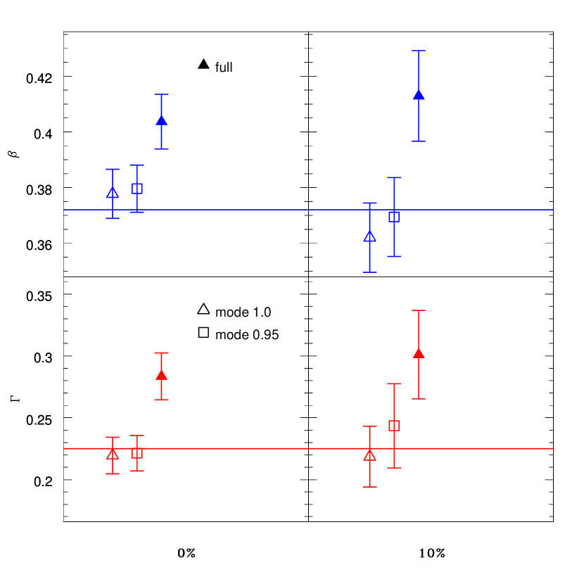
Figure 3: The same as fig 1 with different cosmological parameters ($\Gamma=0.255$, $\beta=0.372$).

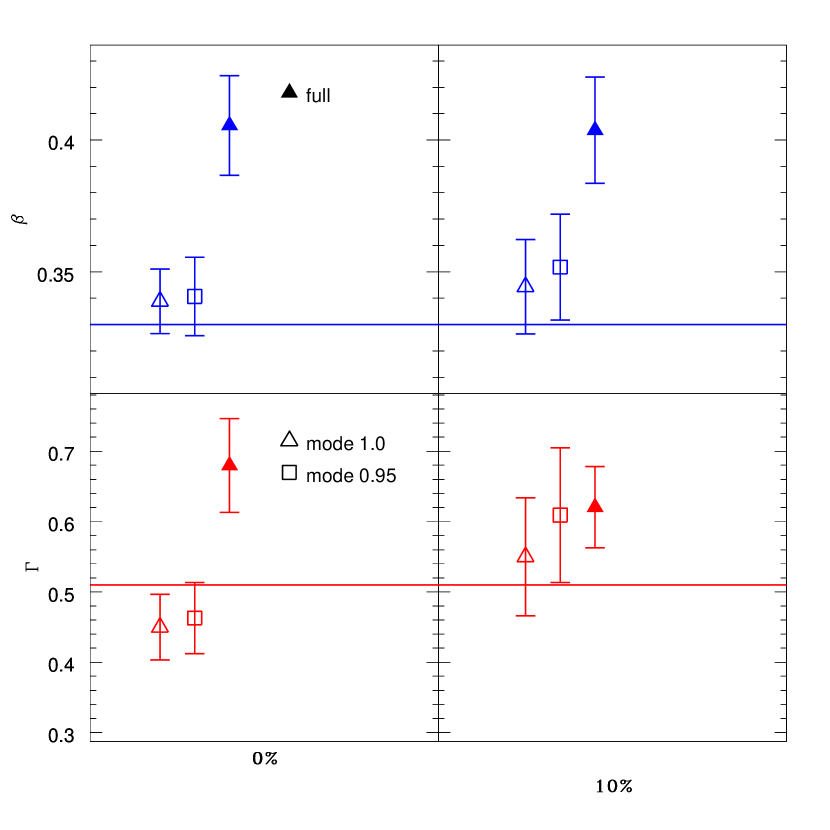
Figure 4: The same as fig 1 with different cosmological parameters ($\Gamma=0.515$, $\beta=0.325$).

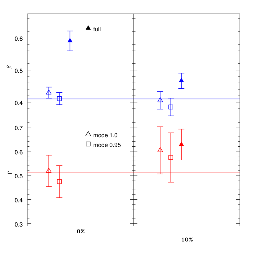
Figure 5: The same as fig 1 with different cosmological parameters ($\Gamma=0.51$, $\beta=0.41$).

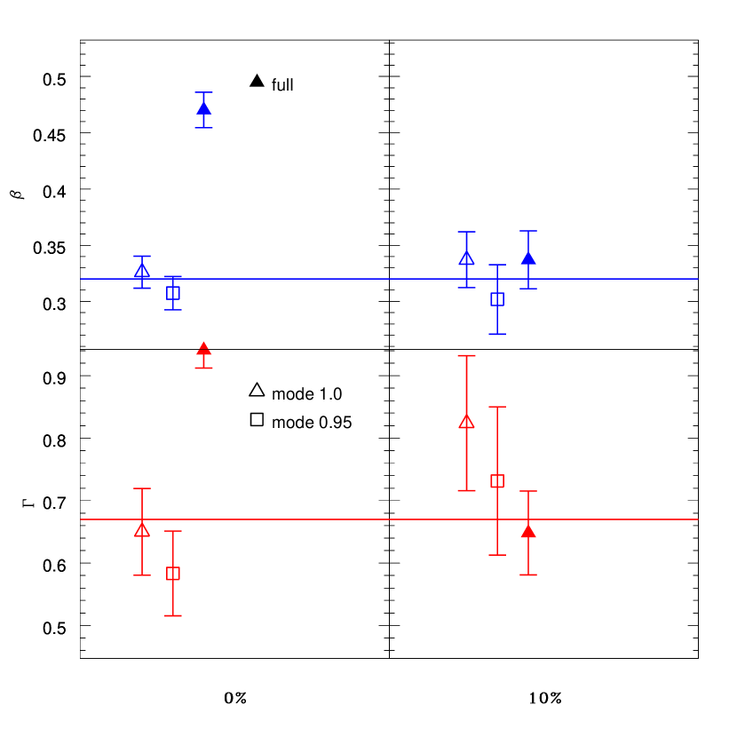
Figure 6: The same as fig 1 with different cosmological parameters ($\Gamma=0.667$, $\beta=0.32$).

As was discussed in the text, the reason for the full analysis failure to recover the “true” parameters when the mode analysis succeeds so well can be shown by looking at the window functions themselves. In fig. 7 we show the window functions corresponding to the five lowest eigenvalues and lowest noise (lower left panel). Clearly, these probe only large scales. As we move up the panels we see the window functions with larger noise components not removed, whereas when we move to the right we see window functions corresponding to larger eigenvalues. Here the reasons for the particular choices for our criteria Eqs. (10) and (12) become clear. As the eigenvalues or the noise level become large, the window functions generally probe more small scale and less of large scale modes. Since we are primarily interested in large scale information, discarding the noisy, high $\lambda$ modes allows us to discard small–scale signal that might interfere with with our analysis.

One more advantage the formalism provides is efficiency. For a catalog of $\approx 1,000$ galaxies it takes the mode analysis about one hour CPU time, whereas it takes the full analysis about seven hours to complete. The differences are more dramatic for larger surveys: A 5,000 galaxy catalog completes in about 30 hours with the mode analysis and about 1,300 hours of CPU time for the full analysis. All runs were done on the Origin2000 at the NCSA, University of Illinois, Urbana–Champaign.

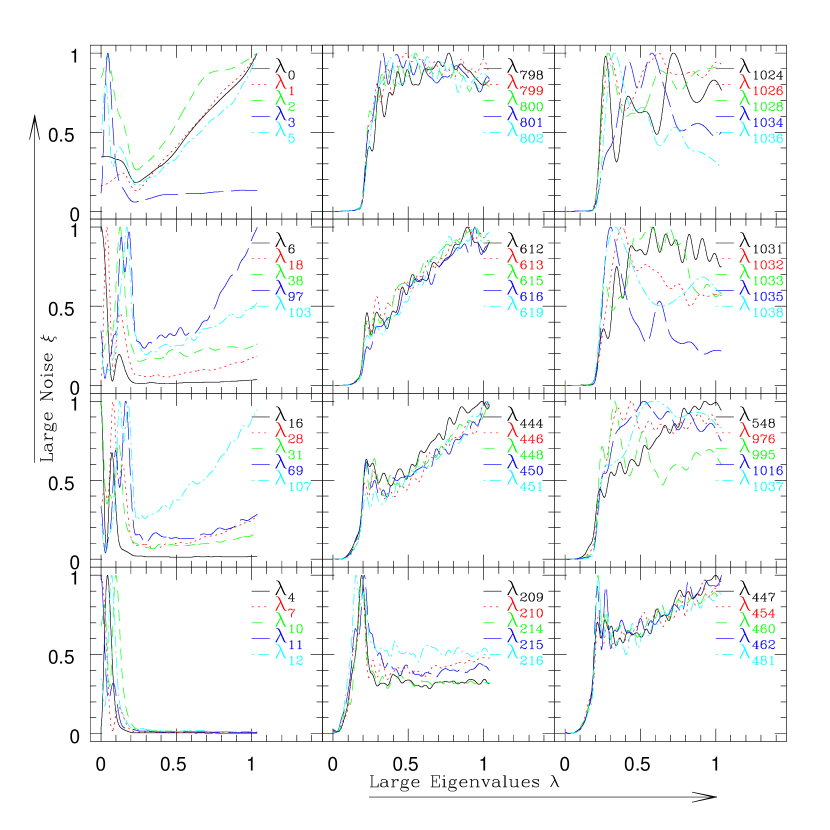
Figure 7: The window functions from top to bottom corresponding to noise in the ranges of $0.98<\xi$, $0.95<\xi<0.98$, $0.9<\xi<0.95$ and $\xi<0.9$ respectively, and across from left low, med and high eigenvalues $\lambda$ respectively. We can clearly see that the low eigenvalue low noise window functions (lower left panel) probe large scale (small $k$), whereas higher noise, larger eigenvalue window functions (up and to the right) correspond to smaller scales probes. Further, the high noise window functions probe scales that are hard to model as are those with large eigenvalues.

As was mentioned in the analysis (Sec. 3) there is a general correlation between the $n^{\rm th}$ moment’s eigenvalue $\lambda_{n}$ and the noise $\xi_{n}$ associated with it (dots in Fig. 8). As can be seen in the figure, the correlation is not perfect, that is, there are low eigenvalues with large noise component, but in general as we move to larger eigenvalues (large $n$) the noise component is larger. The line in the figure represents the running mean of the noise which shows clearly the correlations between the noise and the eigenvalue.

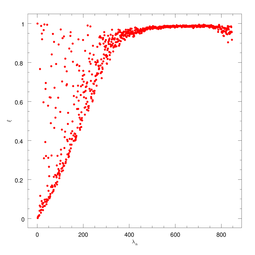
Figure 8: The noise $\xi$ (Eq. 14) as a function of the rank $n$ of the eigenvalue $\lambda_{n}$ (Eq. 12) (shown as dots). On the average there is an excellent correlation between the rank and the noise component.

In Fig. 9 we show the contours that contain 68% and 94% of the total likelihood for six typical catalogs. The diamond shows the maximum likelihood results, whereas the asterix in each panel shows the “true” values of the parameters. These contours allow us to estimate the uncertainty in the maximum likelihood values obtained from the analysis of a single catalog, as is the case when analyzing observational data. From the figures it is clear that the uncertainties obtained in this way are comparable to those we get from the Monte–Carlo simulations. In general, when we try to test the reliability of results from an observational data set, we apply our formalism to mock catalogs extracted from N–body simulations as was done here. This compatibility between the uncertainties obtained in two different ways gives us confidence that using the likelihood contours will give us an accurate assessment of the uncertainties of our maximum likelihood values when we apply our method to real catalogs.

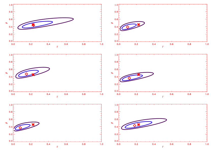
Figure 9: Maximum likelihood contours from six typical mock catalogs. The contours are the 68% and 94% likelihood lines. This shows the expected uncertainties in the analysis of one catalogs. In most cases the uncertainties in the estimated values of the parameters $\Gamma$ and $\beta$ are of comparable sizes to the monte carlo errorbars presented in figures 1–6.

6 Conclusions

We have described the power and elegance of a new statistic that was designed and formulated in order to address a crisis in the analysis of proper distance cosmological surveys. We have shown that our formalism mostly overcomes the problems with the traditional analysis of the data. Whereas the full maximum likelihood analysis tends to overestimate the values of the parameters that describe the power distribution on large scale, our mode analysis makes very accurate estimates of these parameters.

The formalism presented here assumes Gaussian statistics. The natural question should be: Can the deviations from Gaussianity caused by the collapse of perturbations interfere with the removal of small scale power and introduce additional unpredictable biases? As the results in Sec. 5 indicate, deviations from Gaussianity do not have a measurable effect and the effectiveness of filtering small–scale power is unbiased. Further, we have explored in detail such issues as moment and noise selection, the window functions’ effectiveness and criteria for which modes to keep.

As was shown in Paper I and in more detail here, the formalism we presented is highly adaptive and versatile. It can be applied surveys with any geometry and density, and since it retains maximum information should be particularly useful for sparse data such as that obtained in cluster peculiar velocity surveys. Overall, we consider this method to be a significant improvement over previous methods used for the analysis of peculiar velocity data.

References

- Aghanim & G rski (2001) Aghanim, N. & G rski, K. M. 2001, A&A, 374, 1A
- Bardeen et al. (1986) Bardeen, J. M., Bond, J. R., Kaiser, N. & Szalay, A. S. 1986 ApJ 304 15
- Branchini, Plionis & Sciama (1996) Branchini, E., Plionis, M. & Sciama, D.W. 1996 ApJ, 461, L17
- Colless etal (2001) Colless, M., Saglia, R. P., Burstein, D., Davies, R.L., McMahan, R.K. & Wegner, G., 2001, MNRAS 321, 277
- da Costa et al. (1996) da Costa, L.N., Freudling, W., Wegner, G., Giovanelli, R., Haynes, M.P., & Salzer, J.J. 1996, ApJ, 468, L5
- Feldman & Watkins (1994) Feldman, H. A. & Watkins, R., 1994, Theoretical expectations bulk flows in large–scale surveys, ApJ 430 L17–20.
- Feldman & Watkins (1998) Feldman, H.A. & Watkins, R. 1998, A New Approach to Probing Large–Scale Power with Peculiar Velocities, ApJ 494 L129–132
- Freudling et al. (1999) Freudling, W. et al. 1999 Large-Scale Power Spectrum and Cosmological Parameters from SFI Peculiar Velocities ApJ 523 1
- Hudson et al. (1999) Hudson, M. J., Smith, R. J., Lucey, J. R., Schlegel, D.J. & Davies, R.L., 1999 A Large–Scale Bulk Flow of Galaxy Clusters, ApJ 512 L79.
- Kendall & Stuart (1969) Kendall, M. G. & Stuart, A. 1969 The advanced Theory of Statistics Vol. 2, London: Grifin.
- Kenney & Keeping (1954) Kenney, J.F., & Keeping, E.S. 1954, Mathematics of statistics, New York, Van Nostrand company 3rd ed.
- Lauer & Postman (1994) Lauer, T. & Postman, M. 1994 ApJ. 425 418–38
- Melott (1986) Melott, A., 1986 Comment on “Nonlinear Gravitational Clustering in Cosmology”, Phys. Rev. Lett. 56 1992.
- Melott, Weinberg & Gott (1988) Melott, A., Weinberg, D. H., & Gott, J. R. III, 1988 The Topology of Large Scale Structure II: Nonlinear Evolution of Gaussian Models ApJ 328 50.
- Melott & Shandarin (1993) Melott, A. L. & Shandarin, S. F., 1993, Controlled Experiments in Cosmological Gravitational Clustering ApJ 410 469–481
- Riess, Press & Kirshner (1995) Riess, A. G., Press, W. H., & Kirshner, R. P. 1995, ApJ, 438, L17
- Tegmark, Taylor & Heavens (1997) Tegmark, M., Taylor, A.N. & Heavens, A.F., 1997, ApJ 480 22–35
- Watkins & Feldman, (1995) Watkins, R. & Feldman, H. A., 1995, Interpreting New Data on Large–Scale Bulk Flows, ApJ 453 L72–76.
- Watkins et al. (2002) Watkins, R., Feldman, H. A., Chambers, W., Gorman, P. & Melott, A., 2002, Optimal Moments for the Analysis of Peculiar Velocity Surveys ApJ 564 534–541
- Yang et al. (2001) Yang, X. H., Feng, L. L., Chu, Y. Q., & Fang, L. Z. 2001 Measuring Galaxy Power Spectrum. III. ApJ 560 549
- Zaroubi et al. (2001) Zaroubi, S. et al. 2001 MNRAS 326 375
- Zehavi & Dekel (2000) Zehavi, I & Dekel, A., 2000 Cosmological Parameters and Power Spectrum from Peculiar Velocities. In the proceedings of the Cosmic Flows Workshop, Victoria, Canada, 2000, ed. S. Courteau, M. Strauss & J. Willick, ASP series.
- Zel’dovich (1970) Zel’dovich Ya.B. 1970, A&A, 5, 84