Resolving the Microlens Mass Degeneracy for Earth-Mass Planets

Abstract

Of all planet-finding techniques, microlensing is potentially the most sensitive to Earth-mass planets. However, microlensing lightcurves generically yield only the planet-star mass ratio: the mass itself is uncertain to a factor of a few. To determine the planet mass, one must measure both the “microlens parallax” $\tilde{r}_{\rm E}$ and source-lens relative proper motion $\mu_{\rm rel}$. Here we present a new method to measure microlens masses for terrestrial planets. We show that, with only a modest adjustment to the proposed orbit of the dedicated satellite that finds the events, and combined with observations from a ground-based observing program, the planet mass can be measured routinely. The dedicated satellite that finds the events will automatically measure the proper motion and one projection of the “vector microlens parallax” ($\tilde{r}_{\rm E},\phi$). If the satellite is placed in an L2 orbit, or a highly elliptical orbit around the Earth, the Earth-satellite baseline is sufficient to measure a second projection of the vector microlens parallax from the difference in the lightcurves as seen from the Earth and the satellite as the source passes over the caustic structure induced by the planet. This completes the mass measurement.

1. Introduction

Among all proposed methods to search for extra-solar planets, only microlensing has the property that the intrinsic amplitude of the planetary signature remains constant as the planet mass decreases. Hence, with the notable exception of pulsar timing (Wolszczan, 1994), microlensing can in principle probe to lower masses than any other technique. A microlensing space mission that was of similar scale to the transit missions Kepler and Eddington or to the astrometry satellite Space Interferometry Mission (SIM) would be sensitive to Mars-mass companions (Bennett & Rhie, 2002), a decade or two below these other techniques. Furthermore, any microlensing detections of terrestrial planets are expected to be at significantly higher signal-to-noise ratio (S/N), and thus will be more robust to unforeseen systematic errors. Hence, microlensing can potentially play a major role in determining the frequency of terrestrial planets around main-sequence stars. An accurate assessment of this frequency is a key requirement for the design of the Terrestrial Planet Finder, which will ultimately take images and spectra of such planets.

Unfortunately, while microlensing can detect planets of very low mass, there has not seemed to be any way to measure the masses of those planets to better than a factor of a few: although microlensing light curves automatically yield the planet-star mass ratio $q=m_{p}/M$, the stellar mass itself is unknown due to the classic microlensing degeneracy. This degeneracy arises from the fact that among the three microlensing “observables”, the Einstein timescale $t_{\rm E}$, the angular Einstein radius $\theta_{\rm E}$, and the projected Einstein radius $\tilde{r}_{\rm E}$, only $t_{\rm E}$ is routinely extractable from the microlensing light curve. These three observables are related to the three underlying physical parameters, $M$, $\pi_{\rm rel}$, and $\mu_{\rm rel}$, by

$$t_{\rm E}={\theta_{\rm E}\over\mu_{\rm rel}},\quad\theta_{\rm E}=\sqrt{4GM\pi_{\rm rel}\over c^{2}\,{\rm AU}},\quad\tilde{r}_{\rm E}=\sqrt{4GM\,{\rm AU}\over c^{2}\,\pi_{\rm rel}}.$$ (1)

Here, $\pi_{\rm rel}$ and $\mu_{\rm rel}$ are the source-lens relative parallax and proper motion. To determine the mass would require measurement of the other two observables: $M=(c^{2}/4G)\tilde{r}_{\rm E}\theta_{\rm E}$. To date, $\tilde{r}_{\rm E}$ and $\theta_{\rm E}$ have been measured for only about a dozen events each out of the more than 1000 so far discovered, and only for one event have both been measured, thus yielding the mass (An et al. 2002 and references therein).

Although several methods to partially break the microlensing mass degeneracy in special instances have been proposed (Gaudi & Gould, 1997; Rattenbury et al., 2002; Bennett & Rhie, 2002), so far there has only been one idea to do so for a large, representative ensemble of events. Gould & Salim (1992) showed that by combining observations from the ground and the solar-orbiting SIM, one could measure $\theta_{\rm E}$ astrometrically and $\tilde{r}_{\rm E}$ photometrically and so routinely measure the mass. Unfortunately, this technique cannot be applied to terrestrial-planet microlensing events, even in principle. Terrestrial planets can only be detected in events of main-sequence source stars. For giant sources, the planetary microlensing pattern would be much smaller than the source and so would be undetectable (Bennett & Rhie, 2002). Because of its small aperture, SIM cannot observe Galactic-bulge main-sequence stars to the required precision.

Here we present a new method to measure microlens masses for terrestrial planets. The method requires only a modest adjustment to the orbit of a microlensing planet-finder satellite and combining its observations with a ground-based observing program.

2. Microlensing Parameters from a Single Observer

To understand how $\tilde{r}_{\rm E}$ and $\theta_{\rm E}$ can both be measured for terrestrial planets, one should first take a careful inventory of what parameters are automatically measured from planetary microlensing events detected from a planet-finder satellite.

From the width, height and peak time of the underlying event due to the primary, one obtains the three standard microlensing parameters $t_{\rm E}$, $u_{0}$, and $t_{0}$, where the latter two are the dimensionless impact parameter and time of maximum (Paczyński, 1986). In addition to these usual three parameters, one additional parameter of the primary event can also be routinely measured: the parallax asymmetry $\gamma$. The Earth’s acceleration during the event induces parallax effects on the lightcurve. If the event lasts a substantial fraction of a year, then these effects can be used to measure both components of the vector microlens parallax (Gould, 1992). However, for more typical short events, the effect reduces to an asymmetry in the light curve (Gould, Miralda-Escudé & Bahcall, 1994). This parallax asymmetry is in effect a projection of the full vector parallax, and as such is described by a single parameter, $\gamma$,

$$\gamma\equiv a_{\oplus}{t_{\rm E}\over\tilde{v}}\cos\psi\cos\phi,\quad\tilde{v}\equiv{\tilde{r}_{\rm E}\over t_{\rm E}},\quad a_{\oplus}\equiv{4\pi^{2}\,{\rm AU}\over\rm yr^{2}}.$$ (2)

Here ${\rm AU}\cos\psi$ is the length of the Earth-Sun separation projected onto the plane of the sky, $\phi$ is the angle between the source trajectory and this projected separation, and $\tilde{v}$ is the source-lens relative speed projected onto the observer plane. For the typical timescales and projected velocities of events toward the Galactic bulge, $t_{\rm E}\sim 20~{}{\rm days}$ and ${\tilde{v}}\sim 800~{}{\rm km\,s^{-1}}$, the parallax asymmetries would appear to be unmeasurable small, $\gamma\lesssim 10^{-2}$. However, high-cadence $(f\sim 144\,\rm day^{-1})$, high-precision ($\sigma_{\rm ph}\sim 0.01\,\rm mag$) continuous photometric monitoring is required to detect terrestrial planets in the first place (Bennett & Rhie, 2002). As a by-product of such photometry, it should be possible to measure such small parallax asymmetries. Gould (1998) showed that $\gamma$ can be measured with S/N

$${|\gamma|\over\sigma_{\gamma}}=12\biggl{(}{\sigma_{\rm ph}\over 0.01}\biggr{)}^{-1}\biggl{(}{f\over 144\,\rm day^{-1}}\biggr{)}^{-1}\biggl{[}{S(u_{0})\over 3}\biggr{]}^{-1}$$ (3)

$$\times\biggl{(}{\tilde{v}\over 800\,{\rm km\,s^{-1}}}\biggr{)}^{-1}\biggl{(}{t_{\rm E}\over 20\,\rm days}\biggr{)}^{3/2}{|\cos\psi\cos\phi|\over 0.5},$$

where for observation streams beginning and ending well beyond the event, $S$ varies monotonically from $S(0)=2.1$ to $S(0.7)=4.4$. Thus except near June 21 when $\cos\psi\sim 0.1$ for observations toward the Galactic bulge, and except for extremely short events, it should be possible to routinely measure $\gamma$ with good S/N.

For all planetary events, it is generally possible to measure an additional three parameters. Planets generally induce a short-duration deviation to an otherwise unperturbed standard microlensing event. From the duration, peak time, and size and shape of the planetary perturbation, one obtains the planet-star mass ratio $q$, the angle $\alpha$ of the planet-star projected separation relative to the source trajectory, and the angular planet-star separation in units of $\theta_{\rm E}$ (Gould & Loeb, 1992).

Finally, for terrestrial planets it should be possible to routinely measure one additional parameter: $\rho_{*}\equiv\theta_{*}/\theta_{\rm E}$, where $\theta_{*}$ is the source radius. Since $\theta_{*}$ can be determined from the dereddened color and magnitude of the source (see e.g., fig. 10 from An et al. 2002), this would yield $\theta_{\rm E}$. This ratio can be measured whenever the source passes over a magnification pattern with structure on scales $\lesssim\rho_{*}$. In particular, for planetary events, Gaudi & Gould (1997) find that it can be measured provided that $\rho_{*}\gtrsim 0.3q^{1/2}$, which corresponds to,

$$m_{p}\lesssim 4\,M_{\oplus}\biggl{(}{\theta_{*}\over r_{\odot}/R_{0}}\biggr{)}^{2}\biggl{(}{\pi_{\rm rel}\over 40\mu\rm as}\biggr{)}^{-1},$$ (4)

where $r_{\odot}/R_{0}$ is the angular size of a solar-type star at the Galactocentric distance. Note that it is also possible to measure $\rho_{*}$, and thus $\theta_{\rm E}$, from events due to higher-mass planets if the source crosses the planetary caustic.

3. Parameters from Two Observers and Degeneracy Resolution

From satellite measurements alone (§ 2), most of the pieces are already in place for terrestrial planet mass measurements. Since both $\theta_{\rm E}$ and one combination of the vector microlens parallax $(\tilde{r}_{\rm E},\phi)$ can already be measured, all that is required is a measurement of another combination of $(\tilde{r}_{\rm E},\phi)$.

It is well known that $\tilde{r}_{\rm E}$ can be measured by observing an event simultaneously from two telescopes that are significantly displaced from each other. Here ‘significantly’ means that the light curve appears measurably different from the two observatories. In other words, the magnification pattern being probed must have structure on a scale that, when projected to the observer plane, is comparable to the separation of the observers. For typical primary lensing events toward the Galactic bulge, the projected scale of the magnification structure is ${\tilde{r}_{\rm E}}\sim 8~{}{\rm AU}$, and so the observers must be separated by at least $O({\rm AU})$. Thus, by observing the event simultaneously from telescopes on the Earth and in solar orbit, one could routinely measure $\tilde{r}_{\rm E}$ (Refsdal, 1966; Gould, 1995).

Therefore, at first sight, the solution appears simple: just put the microlensing satellite in orbit around the Sun and carry out simultaneous observations from the ground. Unfortunately, the huge data stream from the continuous monitoring of $O(10^{9})$ pixels required to detect the planets (Bennett & Rhie, 2002) make this impossible unless there are major breakthroughs in satellite telemetry. The satellite must stay reasonably close to the Earth to transmit these data efficiently.

However, two factors combine to make feasible microlens parallax measurements from short baselines for events with terrestrial planets. First, one component of the vector microlens parallax is already measured for these events because of the extremely high overall S/N required to detect them. See § 2. Second, the planetary perturbation has structure on scales that are smaller than the primary Einstein ring by a factor of $\sim q^{1/2}$. Therefore, two observers need only be separated by of order the scale of the structures, not the whole Einstein ring (Hardy & Walker, 1995; Gould & Andronov, 1999; Graff & Gould, 2002). For planetary events, the perturbed regions of the Einstein ring typically lie on a line along the planet-star axis and have a width of order $q^{1/2}\tilde{r}_{\rm E}$. The satellite will cross this line at a time that differs from the Earth crossing by $\Delta t$. Figure 1a shows the geometry. By applying the Law of Sines, one finds

$$\Delta t=(q^{1/2}t_{\rm E}){d_{\rm sat}\over q^{1/2}\tilde{r}_{\rm E}}\,{\sin(\phi+\beta-\alpha)\over\sin\alpha},$$ (5)

where $d_{\rm sat}$ is the distance to the satellite, $\alpha$ is the known angle between planet-star axis and the source trajectory, $\beta$ is the known angle between the Earth-Sun and Earth-satellite axes, both projected on the sky, and $\phi$ is the (a priori) unknown angle between the Earth-Sun axis and the source trajectory. Combining equations (2) and (5), one obtains an explicit expression for $\phi$,

$$\tan\phi={\Delta t\over\gamma}\,{a_{\oplus}t_{\rm E}\sin\alpha\cos\psi\over d_{\rm sat}\cos(\beta-\alpha)}-\tan(\beta-\alpha),$$ (6)

and by means of equation (2) an explicit expression for $\tilde{v}$ as well.

The first term on the right-hand side of equation (5) is roughly the duration of the perturbation, the second term is the dimensionless ratio of the Earth-Satellite separation to the width of the perturbation, while the third term is of order unity. Hence, $\Delta t$ can be measured with a fractional precision $\sigma(\Delta t)/\Delta t\sim(\tilde{r}_{\rm E}q^{1/2}/d_{\rm sat})/(\Delta\chi^{2})^{1/2}$, where $\Delta\chi^{2}$ is the square of the S/N with which the perturbation is detected from the weaker observatory (probably the ground). The proposed planet detection threshold from space is $\Delta\chi^{2}=160$, but the expected distribution has a long tail toward larger values, so that half the detections have $\Delta\chi^{2}>800$ (Bennett & Rhie, 2002). Thus, $\Delta t$ could be measured with reasonable precision for a significant fraction of events provided that the satellite was not more than a few times closer than the size of the planetary Einstein ring, $q^{1/2}\tilde{r}_{\rm E}$, and that the ground-based observations were not more than a few times worse than the satellite observations. In addition, the separation cannot be more than a few planetary Einstein radii or the Earth will pass outside the region of the planetary perturbation. To target Earth-mass planets, the separation should therefore be

$$d_{\rm sat}\sim\sqrt{4GM_{\oplus}\,{\rm AU}\over c^{2}\,\pi_{\rm rel}}=0.025\,{\rm AU}\biggl{(}{\pi_{\rm rel}\over 40\,\mu\rm as}\biggr{)}^{-1/2}.$$ (7)

A near optimal solution would seem to be to place the satellite in L2 orbit, which lies at $0.01\,{\rm AU}$ in the anti-Sun direction. However, while data transmission is $10^{4}$ times more efficient from L2 than from an AU, that still might not be efficient enough.

A plausible alternative approach would then be to put the satellite in a highly elliptical orbit with period $P\sim 1\,$month. It would spend the majority of its time near $2a\sim 0.005\,{\rm AU}$, adequate for Earth-mass and lighter planets. During the brief perigee each month it could focus on highly efficient data transmission. Because of this large semi-major axis, the orbit would have to be well out of the ecliptic to avoid gravitational encounters with the Moon, but not so far out that the orbit destablized and crashed into the Earth. In fact, it might be difficult to find such long-term stable orbits, but the satellite could be ejected into solar orbit at the end of its mission with a boost at perigee of only $\Delta v\sim 100\,\rm m\,s^{-1}$, thereby evading the requirement for long-term stability.

One potential concern is that if the satellite is anywhere in the ecliptic (including L2), then $\beta=0^{\circ}$ (or $180^{\circ}$). Microlensing is most sensitive to planets close to the peak of the event. At the peak itself, $\alpha=90^{\circ}$. Therefore, near the peak both terms in equation (6) would be very large, which would in effect magnify the observational errors. However, we find from simulations that the enhanced sensitivity at $\alpha=90^{\circ}$ does not imply a tight clustering of events at this value. Rather the distribution is extremely broad, so there is only a marginal cost to having the satellite in the ecliptic.

4. Discussion

For typical relatively short events, the parallax asymmetry is quite weak and is only detectable because of the satellite’s high cadence and S/N. Thus, one must worry about systematic effects. Gould (1998) identified three such effects not specific to terrestrial observers: variable sources, binary sources, and binary lenses. Because of the long high-quality data stream, the source can easily be checked for low levels of variability. While there may be occasional stars that vary over a few months but not otherwise over several years, the fraction of such stars is not likely to be large and can be measured from the prodigious supply of data on “stable” stars. A binary companion to the source star would have to be separated by 2 or 3 $\theta_{\rm E}$ and have a flux ratio of $\sim\gamma\sim 1\%$ to reproduce the magnitude and shape of a parallax asymmetry. Although additional flux at this level would be evident from a fit to the microlensing event itself, it would not be distinguishable from light from the lens star. However, one could check for consistency between the amount of blended light and the mass and distance to the lens as determined from the parallax asymmetry. Further, if the source is really a binary, high-resolution spectroscopy could uncover of order $10\,{\rm km\,s^{-1}}$ radial velocity variations over time. Binary lenses can also induce asymmetries. There are no studies of the expected rate of these, but for field stars it is probably of the same order as events with pronounced deviations, which is $\sim 5\%$. However, most stars with planets are unlikely to have binary companions within a factor 3 or so of the Einstein radius because they would render the planetary orbit unstable. Thus, while caution is certainly warranted in interpreting lightcurve asymmetries as being due to parallax, systematic effects are unlikely to dominate the signal.

There are two types of checks that can be performed on the mass measurements derived by our method. First, in a significant minority planetary events, the lens can be directly observed (Bennett & Rhie, 2002). The derived mass and relative lens-source parallax ($\pi_{\rm rel}/{\rm AU}=\theta_{\rm E}/\tilde{r}_{\rm E}$) can then be compared to the same quantities as determined from multi-color photometry and/or spectroscopy. Second, in some cases it will be possible to measure not only the offset parallel to the source-lens relative motion $\Delta t/t_{\rm E}$, but also the offset in the orthogonal direction $\Delta u_{0}$. This is because the source will pass over a different part of the planetary perturbation, which will generally yield a slightly different perturbation magnitude (see Fig. 1c). Measurement of both the difference in the magnitude and time of the perturbation then gives the two-dimensional offset in the Einstein ring, and thus a measurement of both components of $(\tilde{r}_{\rm E},\phi)$. This effect is typically weaker than the time offset because the magnification contours as stretched along the planet-star axis, and so requires a higher S/N to detect, but in the cases for which it is detected, the result can be cross checked against the asymmetry measurement.

A microlens planet-finding satellite with parallax capabilities would have a number of other applications. First, it would automatically make precise mass measurements on all caustic-crossing binaries (Graff & Gould, 2002). Second, although it would not measure masses for the majority of larger planets such as gas giants, it would do so for the significant minority of cases in which the source passed over the planetary caustic. From a mathematical point of view, these cases are identical to the caustic-crossing binaries analyzed by Graff & Gould (2002). These caustics are substantially larger than the entire perturbation due to an Earth mass planet. Hence, if there are equal numbers of Earth-mass and Jovian-mass planets, the latter will yield the majority of the mass measurements even though the fraction of mass measurements is higher among the former.

Finally, we have so far not given much attention to the problem of organizing the round-the-clock (and so round-the-world) ground-based observations that must complement the satellite observations. Although easier and cheaper than launching a satellite, the effort required for this is by no means trivial. Such a survey would have tremendous potential in its own right and might be undertaken independently of a satellite. We reserve a full discussion of this idea to a future paper.

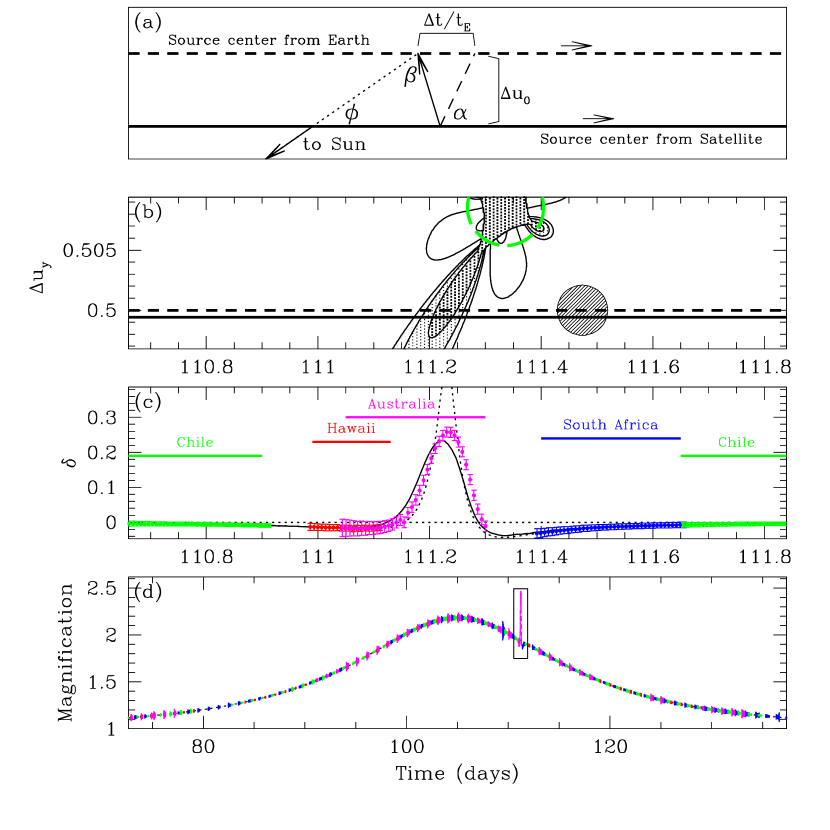
Figure 1.— (a) Geometry of microlens planetary mass measurement. All lines are projected onto the two-dimensional plane of the sky and all distances are scaled to the projected Einstein radius $\tilde{r}_{\rm E}$. Source as seen from the satellite (bold line) travels horizontally at an (a priori unknown) angle $\phi$ relative to the line connecting the Sun and Earth (dotted line), which in turn is at a (known) angle $\beta$ relative to the line connecting the Earth and the satellite. The star-planet axis (thin dashed line) lies at a (known) angle $\alpha$ relative to the source trajectory. As seen from the Earth, the source (bold dashed line) moves on a parallel trajectory but displaced by a distance $d_{\rm sat}/\tilde{r}_{\rm E}$. As a result, the source intersects the perturbation induced by the planet (along the star-planet axis) at a time later by $\Delta t$, corresponding to a fraction $\Delta t/t_{\rm E}$ on an Einstein radius. (b) Contours of constant fractional deviation $\delta$ from the primary lensing event calculated for a point source. Contour levels are $\delta=\pm 5\%,10\%,25\%$; positive contours are shaded. Long-dashed circle shows the planetary Einstein ring radius. The shaded circle shows the size of the source. Horizontal lines are as in panel (a). (c) Planetary perturbations from the primary event as seen from the Earth (points with error bars) and the satellite (solid curve), taking into account of the finite size of the source. The dotted curve is for a point source as seen from the Earth. (d) Primary lensing event with planetary perturbation region outlined. In the example shown, $\phi=30^{\circ}$, $\beta=80^{\circ}$, $\alpha=60^{\circ}$, $\cos\psi=0.93$, $\tilde{r}_{\rm E}=8\,{\rm AU}$, $d_{\rm sat}=0.0054\,{\rm AU}$, $t_{\rm E}=21.58\,$days, $\rho_{*}=2.1\times 10^{-3}$, $q=10^{-5}$, $\pi_{\rm rel}=38\mu{\rm as}$, $\tilde{v}=630{\rm km\,s^{-1}}$, $M=0.3M_{\odot}$, and $m_{p}=qM=M_{\oplus}$.

References

- An et al. (2002) An, J.H., et al. 2002, ApJ, 572, 521
- Bennett & Rhie (2002) Bennett, D.P., & Rhie, S.H. 1996, ApJ, 472, 660
- Bennett & Rhie (2002) Bennett, D.P., & Rhie, S.H. 2002, ApJ, 574, 985
- Gaudi & Gould (1997) Gaudi, B.S. & Gould, A. 1997, ApJ, 486, 85
- Gould (1992) Gould, A. 1992, ApJ, 392, 442
- Gould (1995) Gould, A. 1995, ApJ, 441, L21
- Gould (1998) Gould, A. 1998, ApJ, 506, 253
- Gould & Andronov (1999) Gould, A., & Andronov, N. 1999, ApJ, 516, 236
- Gould & Loeb (1992) Gould, A., & Loeb, A. 1992, ApJ, 396, 104
- Gould, Miralda-Escudé & Bahcall (1994) Gould, A., Miralda-Escudé, & Bahcall, J.N. 1994, ApJ, 423, L105
- Gould & Salim (1992) Gould, A., & Salim, S. 1999, ApJ, 524, 794
- Graff & Gould (2002) Graff, D.S. & Gould, A. 2002, ApJ, 580, 253
- Hardy & Walker (1995) Hardy, S.J. & Walker, M.A. 1995, MNRAS, 276, L79
- Paczyński (1986) Paczyński, B. 1986, ApJ, 304, 1
- Rattenbury et al. (2002) Rattenbury, N. J., Bond, I. A., Skuljan, J., & Yock, P. C. M. 2002, MNRAS, 335, 159
- Refsdal (1966) Refsdal, S. 1966, MNRAS, 134, 315
- Wolszczan (1994) Wolszczan, A. 1994, Science, 264, 538