The BIMA Survey of Nearby Galaxies (BIMA SONG).
II. The CO Data
Abstract
The BIMA Survey of Nearby Galaxies is a systematic imaging study of the 3 mm CO J = 1–0 molecular emission within the centers and disks of 44 nearby spiral galaxies. The typical spatial resolution of the survey is 6″ or 360 pc at the average distance (12 Mpc) of the sample. The velocity resolution of the CO observations is 4 km s-1, though most maps are smoothed to 10 km s-1 resolution. For 33 galaxies, multi-field observations ensured that a region 190″ (D = 10 kpc) in diameter was imaged. For the remaining 11 galaxies, which had smaller optical diameters and were on average farther away, single-pointing observations imaged a 100″-diameter (D = 11 kpc) region. The sample was not chosen based on CO or infrared brightness; instead, all spirals were included that met the selection criteria of 2000 km s-1, -20°, 70°, 70′, and 11.0. The detection rate was 41/44 sources or 93%; of the three nondetections, one (M 81) is known to have CO emission at locations outside the survey field of view. Fully-sampled single-dish CO data were incorporated into the maps for 24 galaxies; these single-dish data comprise the most extensive collection of fully-sampled, two-dimensional single-dish CO maps of external galaxies to date. We also tabulate direct measurements of the global CO flux densities for these 24 sources. For the remaining 20 sources, we collected sensitive single-dish spectra in order to evaluate the large-scale flux recovery. We demonstrate that the measured ratios of flux density recovered are a function of the signal-to-noise of the interferometric data. We examine the degree of central peakedness of the molecular surface density distributions and show that the distributions exhibit their brightest CO emission within the central 6″ in only 20/44 or 45% of the sample. We show that all three Local Group spiral galaxies have CO morphologies that are represented in SONG, though the Milky Way CO luminosity is somewhat below the SONG average, and M31 and M33 are well below average. This survey provides a unique public database of integrated intensity maps, channel maps, spectra, and velocity fields of molecular emission in nearby galaxies. It also lays the groundwork for extragalactic surveys by more powerful future millimeter-wavelength interferometers like CARMA and ALMA.
interferometric–surveys
1 Introduction
In the twenty-five years since the first detection of carbon monoxide in external galaxies (Rickard et al., 1975), astronomers have observed the 3 mm J = 1–0 transition of CO in the centers of several hundreds of galaxies (Verter, 1990; Young & Scoville, 1991; Young et al., 1995; Casoli et al., 1998; Nishiyama & Nakai, 2001; Paglione et al., 2001); these observations form the basis for our statistical understanding of the molecular content of galaxies as a function of parameters like galaxy type and luminosity. Despite an abundance of studies of the amount of CO in galaxies, however, there is still a rather incomplete understanding of the distribution of CO within galaxies. This is because the overwhelming majority of CO observations have been made using single-dish telescopes, the linear resolutions of which are often ten to one hundred times larger than the basic unit in which molecular gas is thought to be organized, the giant molecular cloud (GMC). Also, even for the roughly 200 galaxies that have been observed in multiple pointings with single-dish telescopes, all but a handful have been observed only at select positions along the major and minor axes, rather than in fully-sampled, two-dimensional maps. So far, only a few dozen galaxies have been imaged with the high resolution achievable with an interferometer. The largest published interferometric survey to date is by Sakamoto et al. (1999), who surveyed the central arcminute of 20 nearby spiral galaxies with 4″ resolution using telescopes at the Nobeyama Radio Observatory (NRO) and the Owens Valley Radio Observatory (OVRO).
The BIMA Survey of Nearby Galaxies (BIMA SONG) is the first systematic imaging survey of the 3 mm CO J = 1–0 emission from the centers and disks of nearby spiral galaxies. The basic database that we have produced is a collection of spatial-velocity data cubes for 44 nearby spiral galaxies that show the distribution and kinematics of CO emission at resolutions of a few hundred parsecs ( 6″) and 10 km s-1 over a field of view of typically 10 kpc ( 190″). BIMA SONG was introduced in the recent study by Regan et al. (2001), hereafter Paper I, where we presented initial results for a subsample of 15 spiral galaxies. In this paper, we present data from the full survey of 44 spiral galaxies. Some of the notable features of the BIMA SONG survey are as follows: (1) The sources were not selected based on CO brightness or infrared luminosity. (2) We mosaiced multiple fields for the 33 galaxies with the largest optical diameters, so that the full-width half-power field of view was 190″. This field of view is a full order of magnitude larger in area than was obtained for previous high-resolution surveys. For the 11 galaxies with smaller optical diameters, we used a single pointing of the interferometer to image a region 100″ in diameter. (3) The data have very good sensitivities, with rms noise levels of 23–130 mJy bm-1 per 10 km s-1 channel. These are comparable to the sensitivities obtained by Sakamoto et al. (1999) of 17–110 mJy bm-1 per 10 km s-1 channel over a much smaller field of view. The noise levels are roughly an order of magnitude lower than those of the most extensive single-dish survey, the FCRAO Extragalactic CO Survey (Young et al., 1995). (4) We collected fully-sampled, On-the-Fly (OTF) single-dish maps for 24 of the brightest galaxies and incorporated these data into the SONG maps, so that all of the CO flux is imaged for these galaxies. These maps in themselves comprise the most extensive collection of fully-sampled, two-dimensional single-dish CO maps of external galaxies to date. For the remaining 20 sources, we collected sensitive single-dish spectra in order to evaluate the large-scale flux recovery. (5) All observations, data reduction and analysis were carried out using uniform procedures, so that systematic differences among the resultant maps should be minimized. (6) We are collecting complementary broad-band optical, infrared, H, HI, and radio continuum data so as to have a parallel set of observations for each galaxy. Where available, we have compiled existing data; otherwise, we are obtaining our own new observations. These complementary data will be presented in future SONG papers.
This paper is organized as follows. In §2, we list the sample selection criteria and describe the basic properties of the sample. In §3, we give details of the interferometric and single-dish observations. In §4, we describe the data reduction and calibration. In §5, we present a catalog of the BIMA SONG data in various forms, including channel maps, integrated intensity maps, spectra, and basic velocity fields. In §6, we discuss the CO detection rate for the survey. In §7, we present direct measurements of global fluxes for the 24 OTF sources in the survey. In §8, we discuss the issue of large-scale flux recovery and present measurements for the BIMA SONG sources. In §9, we examine the degree of central peakedness of the molecular surface density distributions. In §10, we consider how the three Local Group spiral galaxies compare with the nearby spirals presented here. We summarize the conclusions in §11. Finally, we have included two appendices in which we give brief descriptions of some deconvolution issues at millimeter wavelengths as well as techniques for combining single-dish data with interferometric data. We note that the data collection, reduction, and calibration procedures were described in considerable detail in Paper I, which is very much a companion to the present paper. Although we present some of the same material here, we have tried to emphasize somewhat different points in the two papers, and we encourage the reader to look to both references for a complete discussion of technical details of the survey. The data from this survey are publicly available (see §11).
2 The BIMA SONG Sample
2.1 Selection Criteria
Sources were selected without reference to CO or infrared brightness. Instead, Hubble type Sa through Sd galaxies were selected with 2000 km s-1; if =75 km s-1 Mpc-1, this corresponds to galaxies with Hubble distances of 27 Mpc. The galaxy inclinations, taken as cos = from axial ratios in the RC3 (de Vaucouleurs et al., 1995), were 70°, so as not to be too edge-on to study azimuthal properties. A minimum declination of -20° ensured that the sources could be observed well from the Hat Creek Radio Observatory in northern California without having too elongated a synthesized beam. To limit the size of the sample, we chose galaxies with apparent total blue magnitudes 11.0. Finally, we used a maximum optical diameter 70′ to exclude one source, M33, which is the subject of a separate BIMA survey (Engargiola et al., 2002). The remaining sources have optical diameters 30′. Using the NASA/IPAC Extragalactic Database (NED)111NED is operated by the Jet Propulsion Laboratory, Caltech, under contract with the National Aeronautics and Space Administration., we identified 44 galaxies meeting all selection criteria. Table 1 lists these 44 sources, which comprise the BIMA SONG sample.
2.2 Properties of the Sample
The BIMA SONG sample includes objects with a range of properties that are of interest for a variety of studies. Spirals with Hubble classifications from Sab to Sd are represented, with roughly one-third of the sample having Hubble type of Sbc and the remaining objects split evenly between earlier and later types (ab:b:bc:c:cd:d = 7:8:14:7:6:2). In Figure 1, we show the distribution of RC3 Hubble types compared with the 486 galaxies from the magnitude-limited Palomar survey of the northern sky (Ho, Filippenko, & Sargent, 1997). Compared to the Palomar survey, the SONG sample has relatively few Sa/Sab galaxies. This is probably a selection effect, since early-type galaxies tend to be found in clusters and are thus farther away on average than the SONG selection criteria allowed. The median distance for the Ho, Filippenko, & Sargent (1997) sample is 17.9 Mpc, compared with 11.9 Mpc for SONG. Nearly two-thirds of the sample are classified optically in the RC3 as barred galaxies, with five SB and 24 SAB bars; the remaining 15 galaxies are optically unbarred. Using the nuclear classifications from the Ho, Filippenko, & Sargent (1997) survey, we note that fourteen of the sources contain nonstellar (Seyfert or LINER) emission-line nuclei, seventeen have starburst (H II) nuclei, and nine show “transition” spectra, with [O I] emission-line strengths intermediate between those of H II nuclei and LINERs. As Figure 2 shows, the nuclear types are distributed in a similar way to those from the Palomar survey. In Figure 3, we show the distribution of arm classifications (AC) as defined (and classified) by Elmegreen & Elmegreen (1987), compared with the Elmegreen & Elmegreen (1987) full sample of 654 spiral galaxies. There are 29 grand-design spirals (AC = 5–12), of which 19 show long arms dominating the optical disk (AC = 9, 12); 13 spirals are flocculents (AC = 1–4), exhibiting fragmented arms that typically lack regular spiral structure. The SONG sample has relatively few galaxies in AC 1 – 5 compared with the Elmegreen & Elmegreen (1987) sample; this may be because the latter sample has more low-luminosity galaxies than does SONG. The galaxies range in distance from 2.1 Mpc to nearly 26 Mpc, with a mean distance of 12.2 5.9 Mpc. The properties of the galaxies are summarized in Table 1.
3 Observations
3.1 BIMA Observations
We carried out BIMA SONG observations from 1997 November through 1999 December using the 10-element Berkeley-Illinois-Maryland Association (BIMA) millimeter interferometer (Welch et al., 1996) at Hat Creek, CA. In all, we included data from about 160 8-hour BIMA SONG tracks as well as about 15 tracks on SONG sources taken by individual team members before 1997 November (Regan, Sheth, & Vogel, 1999; Wong, 2000; Wong & Blitz, 2000). Before 1998 September, the antennas were configured in the then-named C array, which included baselines as short as 7.7 m and as long as 82 m. After 1998 September, we used the current C and D configurations, which together include baselines as short as 8.1 m and as long as 87 m. For all galaxies, we observed the CO J = 1–0 line at 115.2712 GHz. We configured the correlator to have a resolution of 1.56 MHz (4 km s-1) over a total bandwidth of 368 MHz (960 km s-1).
We observed 33/44 of the galaxies (those with R25 200″ as well as three smaller sources) using a 7-field, hexagonal mosaic with a spacing of or 44″; this yielded a half-power field of view of about 190″ or 10 kpc at the average distance of galaxies in the survey. Of these, we observed some galaxies (NGC 0628, NGC 1068, NGC 2903, NGC 3627, NGC 4736, NGC 5033, NGC 5194) with slightly different pointing spacings or additional fields. The remaining 11/44 galaxies were observed with a single pointing, which yielded a field of view of 100″ FWHM. For the multiple-pointing observations, each field was observed for one minute before the telescope slewed to the next pointing. Thus, we returned to each pointing after 8 minutes, which is within the time needed to ensure Nyquist radial sampling of even the longest baselines in the plane; see Helfer et al. (2002).
Table 2 summarizes the observational parameters of the maps, including the number of fields observed, the synthesized beam size in angular and linear dimensions, the velocity binning, and the measured rms noise level in the channel maps.
3.2 NRAO 12 m Observations
We collected over 700 hours of single-dish data from 1998 April through 2000 June using the NRAO 12 m telescope on Kitt Peak, AZ222The National Radio Astronomy Observatory is operated by the Associated Universities, Inc., under cooperative agreement with the National Science Foundation.. We observed orthogonal polarizations using two 256 channel filterbanks at a spectral resolution of 2.0 MHz (5.2 km s-1), and with a 600 MHz configuration of the digital millimeter autocorrelator with 0.80 MHz (2.1 km s-1) resolution as a redundant backend on each polarization. The pointing was monitored every 1-2 hours with observations of planets and strong quasars. The focus was measured at the beginning of each session and after periods during which the dish was heating or cooling. At 115 GHz, the telescope half-power beamwidth, main beam efficiency , and forward spillover and scattering efficiency are 55″, 0.62, and 0.72. To convert from the recorded to , the reader should multiply by / = 1.16. To convert from brightness temperature to units of flux density, the reader should multiply by the antenna gain, or 33 Jy K-1.
For 24 galaxies (Table 2) with the strongest CO brightness temperatures, we observed in On-the-Fly (OTF) mode (Emerson, 1996), where the telescope takes data continuously as it slews across the source. The resultant OTF maps were incorporated into the BIMA maps to create combined BIMA+12m maps that did not have large-scale emission “resolved out” by the interferometer-only observations. The sources with combined maps are identified in the last column of Table 2. For the remaining 20 galaxies, we obtained sensitive position-switched spectra in order to evaluate the large-scale flux recovery. We describe the two observing modes in the following subsections.
3.2.1 On-the-Fly Mapping
The OTF mode minimizes relative calibration errors and pointing errors across a map. In this mode, the actual telescope encoder positions are read out every 0.01 seconds and folded into the spectra, which are read out every 0.1 seconds. We set up a typical OTF map to have a total length of 8′ on a side, which includes a 1′ ramp-up and 1′ ramp-down distance on either side of the 6′ heart of the map, and we alternated scanning in the RA and DEC directions for successive maps in order to minimize striping (cf Emerson & Graeve, 1988). We spent about 30 seconds on each map row and observed a reference position on the sky at the beginning of every second row, calibrating often enough (every 5–15 minutes) so that the measured system temperatures changed by less than a few percent between calibrations. The maps were of course greatly oversampled in the scanning direction; in the orthogonal direction, we spaced the rows by 18″, which slightly oversamples the maps even by the Nyquist criterion (22.4″ at 115 GHz at the 12 m). The output antenna temperatures were recorded as the standard = (ON-OFF)/OFF , where ON is the power measured on source and OFF is the power measured at the reference position on the sky (taken to be the OFF measurement nearest in time to a given ON). For galaxies where the detected CO emission was clearly confined to a region within the OTF map boundaries, we later created a new OFF reference spectrum from the average of roughly 20–40 individual (0.1 second) spectra on either side of each row; although this technique may introduce a systematic, low-level error into the map, it also greatly improves the baseline stability of the spectra. Each individual OTF map took 20 minutes to complete, and we obtained anywhere from 10 to 30 OTF maps to achieve the desired sensitivity; following Cornwell, Holdaway & Uson (1993), we tried to spend enough time on the total-power measurements to match the signal-to-noise ratio of the interferometric observations. In practice, when smoothed to 55″ for direct comparison, the BIMA maps tended to have lower absolute noise levels than the OTF maps by a factor of about two.
Given reasonably stable observing conditions, the relative flux calibration across an individual OTF map should be very good, so that even if the absolute flux scale drifts from map to map, the combined final 12 m map should also have very good pixel-to-pixel calibration. An analysis of well-pointed data over many observing seasons shows that the repeatability of the flux calibration at the 12 m is accurate to better than a 1 uncertainty of 10%. However, the pointing at the 12 m is a more challenging problem. For the OTF data, we were able to crosscorrelate the 12 m data with the BIMA data (§4.3), and we estimate that the absolute pointing accuracy was good to 5″ rms after performing the pointing crosscorrelation. We subtracted baselines based on linear fits to the emission-free channels in the passband, then weighted and gridded the OTF data to an 18″ cell in AIPS. The rms noise levels in the OTF maps were typically 15–20 mK (0.50–0.66 Jy bm-1) per 2 MHz (5.2 km s-1) channel. To allow for some amount of pointing or other systematic errors in the OTF maps, we assign an overall 1 uncertainty of 15% to the flux calibration of the OTF data.
3.2.2 Position Switched Spectra
We observed the remaining 20 galaxies in a simple position-switched mode, where the telescope tracks a specific position on the source for a given integration time (typically 30 seconds), then is pointed to a nearby (typically closer than 30′ in azimuth from the source) reference position to measure the sky brightness. We observed each galaxy at the positions of the BIMA pointings, so that we obtained 7 spectra for the mosaiced BIMA observations and one for the single-pointing BIMA observations. Again, spectra of were recorded as described above. We fitted and removed linear baselines from the spectra using the Bell Labs spectral line reduction package, COMB. The rms noise levels of the spectra were 5–20 mK per 2 MHz (5.2 km s-1) channel.
As with the OTF data, the absolute flux calibration is presumably accurate to a 1 uncertainty of 10%, though this is difficult to measure directly because we were not able to correct for pointing errors, which may be as large as 15–20″. The effect of mispointed data is essentially unpredictable without an independent way of characterizing it (as with the BIMA-12 m pointing crosscorrelation for OTF data described in §4.3). For example, a pointing error of 20″ will cause the measured flux density of a point source to be attenuated by 12%. However, for sources with more complicated structures, the flux density measured at the mispointed position could be higher or lower than the flux density from the desired position. Furthermore, the measured flux density is a function of the observed velocity, so that the spectral line shape may also be in error. We therefore assign a 1 uncertainty of 25% to the flux calibration of the position-switched spectra, keeping in mind that this error is dominated by systematic uncertainty.
The position-switched data from the 12 m telescope are summarized in Table 3, which lists the integrated intensities measured at each position for a given source.
4 Data Reduction and Calibration
A description of the basic data reduction and calibration is given in considerable detail in Paper I. Here, we give a brief overview and detail a few points that were not discussed more fully earlier.
4.1 BIMA Data Reduction
We reduced the BIMA data using the MIRIAD package (Sault, Teuben, & Wright, 1995). We removed the instrumental and atmospheric phase variations from the source visibilities by referencing the phase to observations of a nearby quasar every 30 minutes. The antenna-based frequency dependence of the amplitudes and phases were measured and removed using the BIMA online passband calibration at the time of each track. Using measurements of the rms phase variation over a fixed, 100 m baseline (Lay, 1999), we applied a zeroth-order correction for the atmospheric phase decorrelation (Paper I). The main effect of this correction is to create a dirty beam that more accurately represents the atmospheric-limited response of the interferometer. We set the amplitude scale of the BIMA observations using Mars and Uranus as primary flux calibrators. Following Paper I, we assign a 1 uncertainty to the amplitude calibration of 15%.
We weighted the visibility data by the noise variance and also applied robust weighting (Briggs, 1995) to produce data cubes in right ascension, declination, and LSR velocity. We included shadowed data down to projected baselines of 5 m, after checking for false fringes in the shadowed data; this allowed better measurements of large-scale emission with the modest penalty of 1% attenuation of the measured source amplitude. For most sources, we produced data cubes with a velocity resolution of 10 km s-1, though we used 5 km s-1 for the narrow-line galaxy NGC 0628, and 20 km s-1 for NGC 3031, NGC 4725, and NGC 5033.
For purposes of uniform data reduction, we treated all observations as mosaics, with the 11/44 single-pointing observations a trivial subset of the mosaiced case. Following Sault (1999), we briefly describe the mosaicing process we used as implemented in the MIRIAD package. First, the standard mapping task INVERT produces a “dirty” image of each pointing separately and then combines the separate dirty maps into a linear mosaic by taking a weighted average of pixels in the individual pointings, where the weights are chosen to minimize the theoretical noise and to correct for the primary beam attenuation of the individual pointings. (This “Sault weighting” scheme results in a primary beam function that is flat across most of the mosaiced image but that is attenuated at the edges of the mosaic, so that the noise level does not become excessive there. For the single-pointing observations, the primary beam response is taken to be the usual truncated Gaussian with FWHM of 100″ at 115 GHz.) Because the coverages of the pointings are not identical, the synthesized (“dirty”) beam also differs slightly from pointing to pointing. Together with the Sault weighting scheme, this means that the point spread function (PSF) of the mosaiced image is position-dependent. The INVERT task therefore also produces a cube of beam patterns, one for each pointing, so that the deconvolution can compute the true PSF at any position in the dirty image. We deconvolved the image cubes using a Steer-Dewdney-Ito CLEAN algorithm (Steer, Dewdney, & Ito, 1984); see Appendix A for a discussion of alternative deconvolution schemes and issues concerning the deconvolution. We did not set any CLEAN boxes so as not to introduce any a priori bias as to where we expected emission to be detected. We allowed the deconvolution to clean deeply, to a cutoff of 1.5 times the theoretical rms in each pixel (see Appendix A, final two paragraphs). The deconvolved images were restored in the usual way by convolving the CLEAN solution with a Gaussian with major and minor axes fitted to the central lobe of one plane of the synthesized beam, then adding the residuals from the CLEAN solution to the result.
We performed an iterative, phase-only multi-channel self-calibration on most detected sources. We checked that the source position was not affected by self-calibration by cross-correlating the final BIMA-only map with the a priori phase-calibrated map; in most cases, the source moved by 0.1″ after self-calibration. Instead, the absolute registration of the maps are limited by uncertainties in the phase calibration. Test measurements of two point sources separated by 11° – a typical separation for a source and phase calibrator for BIMA SONG observations – showed that the absolute registration of the maps should be accurate to 0.4″.
4.2 Continuum Emission
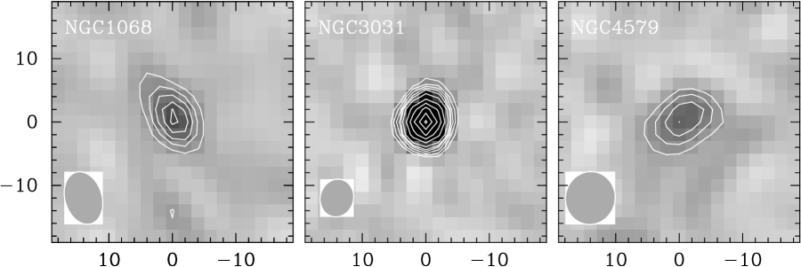
We detected continuum emission at 112 GHz (the lower sideband of the local oscillator) in three sources: NGC 1068 (M 77), NGC 3031 (M 81), and NGC 4579. For all three, we subtracted the continuum from the spectral line data in the visibility plane by fitting a constant to the real and imaginary parts of those channels in the passband that were free of line emission. We list the peak flux density levels of these three galaxies in Table 2 along with 3 upper limits for the remaining sources; the maps of the detected galaxies are shown in Figure 4. We tested to see whether any of the emission was resolved by fitting Gaussians to the three detections. The emission from NGC 1068 was marginally resolved; the deconvolved continuum source size was 7.8″ 2.6″ along position angle 34°, and the integrated source flux density was 59.9 8.1 (formal) 9.0 (systematic) mJy. These results are consistent with previous measurements of the 3 mm continuum in NGC 1068, which is resolved into two components, each of about 40 mJy and separated by about 5″, one to the northeast of the other (e.g. Helfer & Blitz, 1995). The emission from NGC 3031, which is known to have a bright ( 90 mJy), variable, flat-spectrum radio core (e.g. Crane, Giuffrida, & Carlson, 1976; de Bruyn, Crane, Price, & Carlson, 1976), was consistent with that from a point source with a flux density of 161 6 (formal) 24 (systematic) mJy. The emission from NGC 4579, which like NGC 1068 contains a Sy 2 nucleus, appears to be resolved, with a deconvolved source size of 8.7″ 5.5″ along position angle -69° and an integrated source flux density of 45.0 7.5 (formal) 6.8 (systematic) mJy.
4.3 Pointing Crosscorrelation
The implementation of OTF mapping at the NRAO 12 m (§3.2.1) ensures that the internal pointing consistency of an individual OTF map (taken over 20 min) is excellent, even if the overall registration of the map is uncertain. We were further able to cross-correlate either the individual OTF maps or averages of several maps with each other to track slow pointing drifts, allowing OTF maps taken over many hours, days, or even in different observing seasons, to have good internal pointing accuracy.
We performed the cross-correlation using the convolution theorem: the cross-correlation function of the two maps is the inverse Fourier transform of the product of the Fourier transforms of the two input maps. Since the input maps had many channels, we summed the resulting cross-correlation function over all channels and fitted the position of the peak using a two-dimensional gaussian. Using the sum of the cross-correlation function ensures that those channels with the highest values for the cross-correlation are weighted the most.
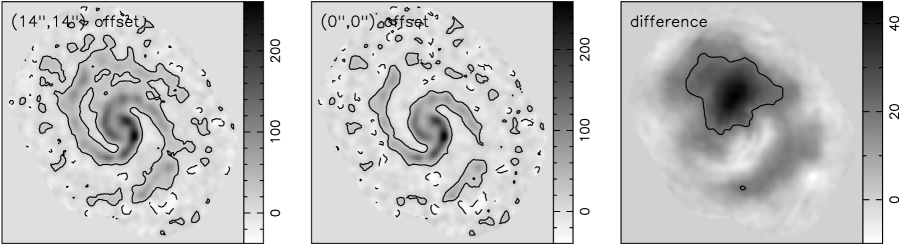
The absolute registration of the 12 m maps was accomplished by cross-correlating the well-pointed average 12 m map with the BIMA map, where the BIMA map was smoothed to match the 55″ resolution of the 12 m at 115 GHz. In performing this crosscorrelation, we had to assume that the extended emission estimated by the deconvolution but not sampled by the interferometer (Appendix A) – that is, the “resolved-out” flux in the interferometer maps – correctly placed the centroid of the emission. A theoretically more robust method, comparing flux density just in the region of overlap, was limited by poor S/N in the overlap region of the 12 m data. In general, the resulting pointing corrections were 5-10″, but some were as large as 20″. If a pointing offset of this magnitude is left uncorrected, it has the effect of inserting a phase shift into the combined map, so that there will be symmetrically placed positive and negative residuals in the final combined map. An example of this is shown in Figure 5, which shows a combined BIMA+12m map of NGC 5194 before (left) and after (middle) correcting a simulated 20″ offset between the 12 m and BIMA maps. The difference between the uncorrected and corrected maps (right) emphasizes the symmetric positive and negative errors introduced in the combined map. The peak error in the difference map is nearly 20% of the peak value in the correct map of the galaxy.
4.4 BIMA and Single Dish Data Combination
For the 24 galaxies with complete OTF mapping from the NRAO 12 m (Table 2, §3.2.1), we combined the BIMA data with the single dish data so that the large-scale emission is accurately imaged. In Appendix B, we discuss different techniques for combining interferometric data with single dish data. For this paper, we used the combination method described in Stanimirovic et al. (1999) (with a CLEAN-based deconvolution instead of their MEM). First, we created a new “dirty” (undeconvolved) map using a linear combination of the BIMA “dirty” map and the OTF map, where the OTF map was tapered by the BIMA primary beam function and resampled onto the same grid as the BIMA dirty map. For the linear combination, we chose to weight the images in inverse proportion to the beam areas. (In principle, one could choose any number of weighting schemes. In practice, however, putting both images on a common temperature scale is the appropriate choice in the relatively low S/N regime of millimeter data, where there may be a significant contribution to the total flux in the residual map; see discussion in Appendix A.) We also created a new “dirty” beam using the same weights for a linear combination of the BIMA synthesized beam and the 12 m beam, where the 12 m beam was assumed to be a truncated Gaussian. We deconvolved the new “dirty” map by the new “dirty” beam using a Steer-Dewdney-Ito CLEAN algorithm as described in §4.1. As with the BIMA-only maps, we restored the final images by convolving the CLEAN solution with a Gaussian (fitted to the central lobe of one plane of the combined “dirty” beam cube) and then adding the residuals from the CLEAN solution to the result.
5 A Catalog of BIMA SONG Data
The full catalog of BIMA SONG figures is available online
at
http://astro.berkeley.edu/~thelfer/bimasong_supplement.pdf
and through the online edition of the Astrophysical Journal at
http://www.journals.uchicago.edu/ApJ/journal.
For each source, the catalog shows the following:
1. (Upper left panel): The distribution of CO integrated intensity (“moment-0”) emission is shown by red contours overlaid on an optical or infrared image of the galaxy. The integrated intensity maps were formed in the following way. First, we created a mask by smoothing the data cube by a Gaussian with FWHM = 20″ and then accepting all pixels in each channel map where the emission was detected at a level above 3 times the measured rms noise level of the smoothed cube. Second, we summed all the emission in the full-resolution data cube after accepting only those pixels that were nonzero in the mask file. Finally, we multiplied by the velocity width of an individual channel to generate a map of integrated intensity in the units of Jy bm-1 km s-1. This smooth-and-mask technique is very effective at showing low-level emission which is distributed in a similar way to the brighter emission in the map. Such low-level distributions are common, since the deconvolution often leaves systematic, positive residuals in the shape of the source (Appendix A), which is almost certainly true emission associated with the source. Another advantage of the smooth-and-mask technique is that it does not bias the noise statistics of the final image, unlike the commonly used method of clipping out low-level pixels in the channel maps. However, the smooth-and-mask method may introduce a bias against any possible compact, faint emission that is distributed differently than the brightest emission.
For each map in the upper left panel, the contours are spaced logarithmically in units of one magnitude, or with levels at 2.51 times the previous level. The starting contour is given in Table 2. The solid blue contour denotes the gain=0.5 contour of the primary beam. For the single-pointing observations (Table 2), the primary beam response is unity only at the center of the map and falls off as a Gaussian function at distances away from the center. For multiple pointing observations, on the other hand, each galaxy has a uniform primary beam function inside a large region bounded by a dashed blue contour; the gain falls from 1 to 0.5 between the dashed and solid blue contours.
2. (Upper middle panel): The same CO integrated intensity emission shown in the upper left panel is shown as black contours overlaid on a false-color representation of the CO emission. The contours are exponentially spaced at half-magnitude intervals, or 1.59 times the previous interval. The starting contour is given in Table 2. The false-color minimum is set to the value of the lowest pixel in the map, which is on average -2.5 Jy bm-1 km s-1. The false-color maximum for all maps is 315 Jy bm-1 km s-1, so that the reader can easily determine the relative strengths of the flux density for the different sources. The FWHM of the synthesized beam is shown near the lower left corner of this box, next to a vertical bar that shows the angular size of 1 kpc at the assumed distance to the source.
3. (Upper right panel): A representative CO velocity field is shown in false color. The fields were generated by taking the mean velocity at each pixel from Gaussian fits as follows. First, a single Gaussian was fit to the spectrum at each pixel in the datacube. The initial estimates for the amplitude and velocity of the Gaussian were taken from the peak of the spectrum at each pixel. The initial estimate for the FWHM of the Gaussian was taken to be 30 km s-1 or 60 km s-1 (the fitting routine was run for both values, and the results for 60 km s-1 were used when the 30 km s-1 fit failed). The Gaussian fits were rejected if the velocity error exceeded 2 channels or if the integrated flux density of the Gaussian was less than , where is the rms noise level in a channel map and is the velocity width of a channel. Finally, the same spatial mask used for the integrated intensity images (described in “upper left panel” above) was applied to the velocity fields. The wedge at the right of each velocity field shows the range and values of the velocities for each galaxy. Velocity contours are overlaid on the false-color images; the contours are spaced at 20 km s-1 intervals, except for the narrow-line galaxies IC 342, NGC 0628, and NGC 3184, which are spaced at 10 km s-1 intervals, and the wide-line galaxies NGC 3368, NGC 4258, NGC 5005, NGC 5033, and NGC 7331, which are spaced at 40 km s-1 intervals.
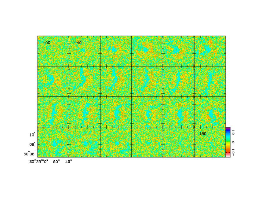
4. (Lower left panel): The individual channel maps are shown over the velocity range of emission. The BIMA SONG data are shown as a false-color halftone, the stretch of which is shown in a wedge to the right of the last panel and which ranges from to 0.75 times the peak value in the channel map. The gain=0.5 contour is shown as a solid blue contour in the upper left panel. The LSR velocities are given for the first, second, and last panels of the map; the velocity width of each channel may be inferred from the difference between the velocities listed in the first and second panels. Where present, light gray contours show emission measured in OTF mapping at the NRAO 12 m telescope. The contours start at 3 , where is the measured rms noise in the 12 m channel map (listed in Table 2), and are spaced by factors of 1.5.
5. (Lower right panel): Spectra comparing the BIMA SONG maps at 55″ resolution are shown along with corresponding 55″ spectra from the NRAO 12 m telescope. For those galaxies mapped with OTF mapping at the 12 m, a grid of spectra is shown overlaid on a grayscale representation of the integrated intensity map. The spectra are spaced by 30″ centered on the tracking center of the source as listed in Table 1; the location of each spectrum is marked by a light blue cross. The red spectrum is the BIMA-only data, smoothed to 55″; the blue is the BIMA+12m combined data, smoothed to 55″, and the green is the 12 m-only data, at its full resolution of 55″. The LSR velocity and flux density scales are shown in a frame around the lower left spectrum. For those galaxies not mapped with OTF mapping at the 12 m, we show instead individual spectra taken at each of the pointing centers of the BIMA mosaic, at (0″,0″), (44″,0″), and (22″,38″). Again, the red spectrum is the BIMA-only data, smoothed to 55″, and the green spectrum is the 12 m-only data.
6 Detection Rate
Since neither CO nor infrared flux density were selection criteria for the SONG sample, it is of interest to see what the detection rate of the survey was. Of the 44 galaxies included, only three or 7% were not detected in line emission. These are NGC 3031 (which was detected in the continuum; see §4.2) and NGC 4699, which were also not detected with the NRAO 12 m telescope, and NGC 3992, which was formally detected in at least one position with the 12 m (Table 3). We note that NGC 3031 (M 81) is a large galaxy with known CO emission at 120″, which is outside our field of view (e.g. Brouillet et al., 1991). This means that 42/44 = 95% of the SONG galaxies have known CO emission.
The high detection rate for CO is not unexpected for a magnitude-limited sample, since optically bright galaxies might be expected to be brighter at all wavelengths. Another contributing factor is likely to be the Hubble type distribution (Figure 1), since Hubble types outside the Sa–Sd range were explicitly excluded, and there are few early-type spirals (Sa–Sab) because the sample is also volume-limited and such galaxies are rarer. For comparison, Young et al. (1995) detected CO in 96% of Sc galaxies, 88% of Sa–Scd galaxies, and 79% of galaxies over all Hubble types. The tendency for CO to be brightest in intermediate-type galaxies can be understood in terms of galactic evolution: early type galaxies such as ellipticals and S0 galaxies have converted most of their gas into stars, whereas late-type galaxies, while gas rich, are generally low in metallicity (Zaritsky, Kennicutt, & Huchra, 1994), and thus less likely to show detectable CO emission.
7 Global Fluxes
The NRAO 12 m OTF data we have collected for 24 SONG sources comprise the most extensive collection of fully-sampled, two-dimensional single-dish maps of external galaxies to date. We have measured the global flux densities directly in these galaxies, without having to rely on model fitting of data at selected positions and the extrapolation of these models to larger radii.
For 19/24 galaxies, we mapped a core square region of 6′6′ with uniform sensitivity; an additional 1′ which was included for a ramp-up or ramp-down distance extends the total region mapped to 8′8′, though the outer 1′ (square) annulus has significantly lower sensitivity than the core region of the map. For NGC 3938, NGC 5033, and NGC 5247, the core region was 5′5′; for NGC 5457, the core region was 7′7′; and for NGC 5194, the core region was 8′12′.
The global flux densities, measured inside the core regions, are listed in Table 4. The integrated flux densities are also shown as a function of the length of a square region over which the flux density was measured in Figure 6. For most of the sources, the flux density at the core length (denoted by the vertical dotted lines) has achieved a plateau, which suggests that there is very little emission from CO at larger regions than measured. For large sources like IC 342, the flux density is clearly still increasing at large ; this is consistent with the known CO distribution of this galaxy, which extends to nearly 15′15′ on the sky (Crosthwaite et al., 2001). Some of the sources, like NGC 4569 and NGC 5005, show a large increase in flux density outside the core region even though the emission appears to have achieved a plateau inside the core region. While it may be that the flux density for these sources truly increases outside the core region, the error bars on the points at large are large enough that the measured points are also consistent with the flux density measured at the core length.
We compare our measured OTF global flux densities with global flux densities derived from model distributions using the FCRAO Survey (Young et al., 1995) in Figure 7. In general, the agreement is very good; the average ratio of the OTF to FCRAO flux density is 1.05, with a standard deviation of 0.19. The worst discrepancies are for the galaxies with the lowest global fluxes, like NGC 3351 and NGC 4258, where the OTF measurements are both 2.2 times higher than the FCRAO flux density, or NGC 3938, where the OTF measurement is 0.53 times the FCRAO flux density. This tendency was also apparent when we compared integrated intensities from the position-switched data from the 12m telescope (Table 3) with those at matched positions from the FCRAO survey: the weaker sources disagreed by as much as a factor of 2, while the stronger sources agreed to within about 20%.
Table 4 also lists the CO luminosity and total CO mass inside the region measured for each OTF source. Assuming a constant CO/H2 ratio of 2 cm-2 (K km s-1)-1, the calculated masses range from 2.4108 M☉ for NGC 4736 to 7.4109 M☉ for NGC 5248; the average of the measured OTF masses is 3.3109 M☉.
8 Flux Recovery
An interferometer is fundamentally limited by the minimum spacing of its elements. Because two elements can never be placed closer than some minimum distance , signals on the sky larger than some size will be severely attenuated. This effect is commonly referred to as the “missing flux” problem. In this section, we present an analysis of the issue of large-scale flux recovery as measured using a comparison of BIMA-only data with the total flux as measured at the NRAO 12 m telescope. We emphasize that for the 24 BIMA SONG maps that incorporate 12 m OTF data into them, the final BIMA SONG maps presented in this paper are not missing any flux. Nonetheless, an analysis of the BIMA-only data for these sources leads to some new results on this technical issue, which are discussed below.
8.1 Imaging Simulations of Large-Scale Flux Recovery
With the BIMA SONG observations for motivation, Helfer et al. (2002) recently presented a study of imaging simulations of large-scale flux recovery at millimeter wavelengths. These simulations showed that the nonlinear deconvolutions that are routinely applied to interferometric maps interpolate and extrapolate to unsampled spatial frequencies and thereby reconstruct much larger scale structures than would be suggested by an analytical treatment of the flux recovery problem. However, Helfer et al. (2002) also showed that fraction of flux density recovered for a given observation is a function of the S/N ratio of the map. This is illustrated in Figure 8, which shows the fractions of total and peak flux densities as a function of the S/N ratio for simulated BIMA observations of sources with widths of 10–40″. For S/N ratios of 10–40, which are typical of individual channels for BIMA SONG maps, we could expect to reconstruct roughly 80–90% of the total flux density of a 10″ source and roughly 30–50% of the total flux density of a 40″ source, whereas for noise-free simulations, BIMA recovers essentially all of the total flux density of a 10″ source and 80% of the total flux density of a 40″ source (see Table 2 in Helfer et al., 2002). The fraction of the peak flux density recovered (bottom panel of Figure 8) is typically somewhat higher than the fraction of total flux density recovered.
8.2 Flux Recovery for BIMA Maps with OTF Data
In each of the 24 galaxies for which we have complete OTF mapping from the NRAO 12 m telescope (Table 2), we were able to make a pixel-by-pixel measurement of the flux recovery of the BIMA-only maps. To do this, we first divided the BIMA data cube by the appropriate (mosaiced or non-mosaiced) primary gain function; we then smoothed the data cube to the 55″ resolution of the 12 m maps. Finally we summed over the planes with emission in order to make a map of integrated intensity. We made the corresponding integrated intensity maps of the 12 m emission and then formed ratio maps of the smoothed BIMA-only maps to the 12 m maps. Finally, we masked the ratio maps to show only those pixels that are non-zero in the masked, clipped moment maps shown in the BIMA SONG catalog in §5, and we clipped outside the original gain=0.5 contour (also shown in the maps in §5). This masking and clipping serves the purpose of eliminating pixels with the highest formal errors in the ratio maps. Given the assigned 1 uncertainty of 15% for the flux density in the BIMA maps and 15% for the 12 m maps, the 1 error in the ratio maps is 21%.
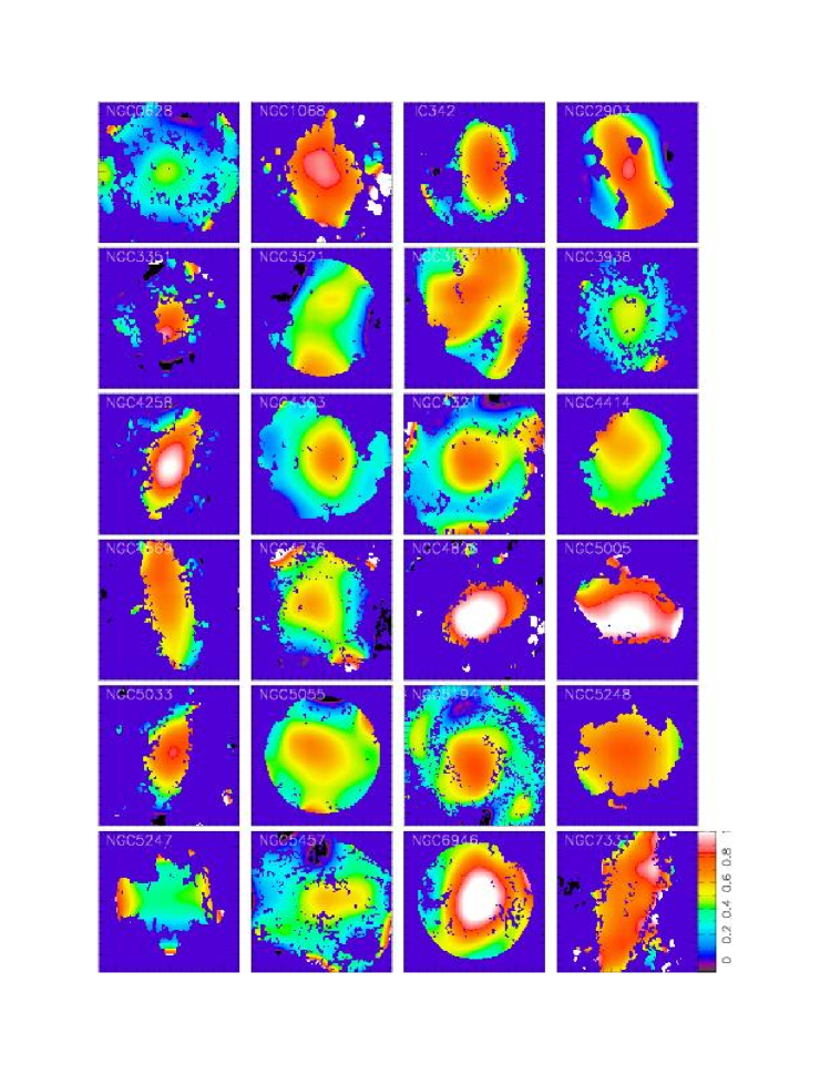
The flux recovery ratio maps are shown in Figure 9. We can see from the figure that there is a remarkable variety in the flux recovery from source to source: for NGC 1068, NGC 4258, NGC 4826, NGC 5005, and NGC 6946, essentially all of the single-dish flux density is recovered by the BIMA maps, at least in the regions of brightest emission. At the other extreme, for NGC 0628, NGC 3938, and NGC 5247, only 30–50% of the total single-dish flux density is recovered over most of the strongest emitting regions. The remaining 16 sources recover intermediate amounts of flux density, with values typically about 70–90% over the brightest regions. Clearly, the ability of any given interferometer to reconstruct structures in a source is very dependent on the source itself.
It is clear from Figure 9 that the fraction of flux density recovered by a given telescope is a function of location within the map. Even for a source like NGC 6946, which has a dominant, centrally concentrated region of emission in the nuclear region which is fully recovered by the interferometer (Figure 9), we can see that away from the nucleus, the fraction of flux density recovered falls to 30–40%. This is also apparent in the grid of spectra shown in the Catalog figure for NGC 6946. This trend is generally apparent (if we exclude galaxies with ring-like emission, like NGC 3521 and NGC 7331): the farther from the nucleus, the less the fraction of flux density recovered. We can attribute this trend to three factors: first, for any given velocity in a data cube, there is a larger region of sky available to emit at locations away from the center of the galaxy rather than at the center (that is, the velocity gradient is largest at the nucleus, which tends to confine emission near the nucleus to small widths in individual channel maps). Second, the tendency is for the brightest emission and best sensitivity to be near the center, so that the S/N ratio is highest in the central region. From Figure 8 and the description of imaging simulations above (§8.1), we would expect the deconvolution to reconstruct less of the total flux in regions of lower S/N. Third, for the BIMA SONG mosaiced galaxies, only the central pointing of the 7-pointing observations had the full benefit the Ekers & Rots (1979) effect. Ekers & Rots (1979) argued that each point measured included contributions from effective baselines as short as , where is the minimum (projected) center-to-center separation of the dishes and is the dish diameter, and they showed that one could effectively extend the sampling inwards to by scanning the telescope over the source. However, for the 26-field mosaic of NGC 5194 as well as the single-pointing observations of NGC 4414 and NGC 5005 (and to a lesser extent, NGC 5248 and NGC 5247), the fraction of flux density recovered still falls as a function of distance from the nucleus. We may conclude that the lack of the required Ekers and Rots sampling for the outer fields of the BIMA SONG mosaics is somewhat less of a valid explanation for the observed trend than the other two factors described above.
The dependence of the flux recovery on the S/N ratio of the interferometric data predicted by the simulations is readily apparent in real data. Figure 10 shows the ratio of total flux recovered as a function of the S/N ratio for each of the 24 galaxies with OTF maps. With the possible exception of NGC 1068, each source clearly shows the predicted trend. (From inspection of the ratio map of NGC 1068 in Figure 9, those pixels with the highest measured ratios probably have the highest formal errors in the ratio as well.)
For the 24 galaxies shown in Figure 9, we have of course incorporated the 12 m OTF data in the BIMA SONG maps so that the total flux density is accurate for these maps. Furthermore, structures larger than 55″ should be accurately represented in the BIMA+12m SONG maps, and structures 20″ should also be accurately represented in the maps. It is difficult to be confident of the accuracy of structures on the intermediate size scales of 20–55″. In all likelihood, these structures are somewhat misrepresented as their attenuated BIMA-only structures sitting atop a smoothed-out 12 m plateau.
8.3 Flux Recovery for BIMA Maps with PS Data
The remaining 20 BIMA-only maps typically have lower S/N ratios than the BIMA+12m maps; this is because CO brightness was a selection criterion in deciding which sources to observe with OTF mapping at the NRAO 12 m. These galaxies were instead observed in a simple position-switched mode at the 12 m. Given the lower S/N ratios, we would expect to reconstruct less flux density than for the brighter sources shown above (§8.1; Helfer et al., 2002).
For the BIMA-only galaxies, we compared integrated intensities of spectra taken with the NRAO 12 m telescope at each of the BIMA pointing centers with the flux density measured in the BIMA-only maps, smoothed to 55″. As with the BIMA+12m maps, in order to compute the ratio of flux density recovered, we first divided the BIMA data cube by the (mosaiced or non-mosaiced) primary gain. We then summed those planes in the smoothed data cube that correspond to the velocity limits of integration in the 12 m spectra. The 12 m and 55″-smoothed BIMA spectra are displayed in the BIMA SONG catalog in §5; the ratios of flux density recovered are also listed in the last column of Table 3 along with their formal uncertainties. Given the assigned 1 systematic uncertainties of 15% in the BIMA maps and 25% in the 12 m spectra (§3.2.2), the systematic 1 error in the ratios are 30%.
Of the 97 positions observed at the 12 m and listed in Table 3, we
detected 55 positions. Of these 55 positions that were detected
at the 12 m, the ratios of the BIMA-55″ flux density to 12 m flux density
are measured at 21 positions with a 2 confidence level.
The ratios for all 55 positions are plotted in Figure 11,
which shows the 21 detected ratios as open squares and the remaining
34 ratios as filled squares.
As the figure shows, there is a clear trend to detect higher ratios
where the S/N of the BIMA data is higher.
Furthermore, as with the BIMA+12m maps, the ratio of flux density recovered
tends to be higher in the central position than in the outer regions
of the mosaic, at least for the brighter galaxies.
We may conclude that, given better S/N measurements, we would likely
be able to reconstruct more flux density than has been measured here.
Furthermore, following Figure 8, we might expect that the peak
flux density that is measured in the BIMA SONG maps is a more reliable
indicator of the flux density in the source than the total flux density
is. This is exemplified in the BIMA and 12 m spectra shown for NGC 3184 in
the BIMA SONG catalog entry (see
http://astro.berkeley.edu/~thelfer/bimasong_supplement.pdf),
where the ratio of peak flux density recovered for the
central region is about 75%; compare this with the ratio of
total flux density recovered of 54% from Table 3.
From the results of Helfer et al. (2002) and from the above examples, it is clear that it is very difficult to conclude whether some or all of the BIMA-only SONG maps are systematically missing large-scale emission, or whether the SONG maps are instead reasonable representations of the sources, albeit at low S/N. It may be reasonable to assume that those maps of galaxies with only compact structure apparent, like NGC 3726 or NGC 4725, may be fairly accurate representations of the sources. Maps of galaxies with clearly extended structures, like NGC 3184 or NGC 4535, are almost certainly missing some of the larger-scale flux density.
9 Do Molecular Distributions Peak at the Centers of Galaxies?
In the FCRAO Extragalactic CO Survey (Young et al., 1995), only 15% of the 193 galaxies observed at multiple positions at 45″ resolution showed molecular distributions that lacked a central peak. In Paper I, we showed that our single-dish data were consistent with this result, namely, that all 15 Paper I galaxies showed single-dish radial profiles that rise monotonically to the nucleus. Thus, it appears that the bulk of molecular gas in nearby spiral galaxies tends to be concentrated within the central 5 kpc.
At 6″ resolution, however, about half of the SONG subsample did not exhibit central peaks (Paper I), a result that was unlikely to have been caused by differences in the two samples. For the full sample, we can quantify the degree of the central concentration by comparing the molecular surface density at the center of the galaxy to the peak molecular surface density in the galaxy. The ratio of central to peak surface brightness should be fairly insensitive to the amount of flux resolved out, so even for the 20/44 maps which lack single-dish data, the ratio should be a valid measure of the central peakedness. We list the peak surface density and the central surface density (taken as the peak within the central 6″ beam) in Table 5, and we show a histogram of the distributions in Figure 12.
As Figure 12 shows, just 20/44 or 45% of the SONG galaxies have their peak molecular surface densities within the central 6″ or 360 pc. At the other extreme, 6/44 or 14% of the galaxies lack any detectable molecular gas within the central few hundred pc. The remaining 18/44 sources show intermediate fractions, where there is detected CO at the center but at a level that is weaker than the peak surface density. We note that two of the galaxies with particularly low fractions – NGC 0628 (0.20) and NGC 5194 (M51, 0.28) are grand-design spirals with two dominant spiral arms that may be traced all the way to the nuclear region. The integrated intensity maps of these galaxies suggest a continuity of the large scale structure down to the 100-pc scales in the nuclear regions of these galaxies, in contrast to galaxies like the Milky Way (§10) or SONG galaxies like NGC 6946, which show central concentrations in the inner 500 pc that are an order of magnitude higher in molecular surface density than are seen in their disks.
10 Comparison with Local Group Morphologies
Galaxies like the Milky Way and M31 produce most of the optical luminosity in the nearby universe because they have luminosities close to the knee in the luminosity function (L∗) (e.g. Binney & Merrifield, 1998). It is reasonable then to ask the following: to what degree are their CO distributions represented in the SONG sample? In this section, we present a basic comparison of Local Group molecular morphologies and brightnesses to those from the survey. We defer any more complex analysis of underlying causes for the morphologies, whether caused by bars or other dynamical considerations (Regan et al., 2002), galaxy luminosity, size, or other factors.
We first determine the characteristic sensitivity of the SONG survey. The typical rms noise is about 58 mJy in a 6.1″ beam when the velocity channels are averaged to 10 km s-1, a velocity resolution comparable to the FWHM linewidth of a GMC in the Milky Way (Blitz, 1993). (The best sensitivity achieved by SONG is a factor of 2.5 lower than this average; see Table 2.) Using a CO/H2 conversion factor of 2 cm-2 (K km s-1)-1, this corresponds to an rms column density sensitivity of 4.6 M☉ pc-2 in each 10 km s-1 velocity channel. Isolated points in the SONG maps are probably not significant at less than 3 or 13.7 M☉ pc-2, but the edges of extended emission are probably reliable at 2 or 9.1 M☉ pc-2. The typical spatial resolution in a 6.1″ beam is 350 pc at the median distance of 11.9 Mpc, but is a factor of 5 smaller for the nearest galaxies. For comparison, the mean surface density of a GMC in the solar vicinity is 50 - 100 M☉ pc-2 (Blitz, 1993), within an area of 2.1 pc2.
The distribution of CO in the Milky Way can be described as having a central molecular disk, a zone of small but indeterminate surface density out to about 3 kpc, increasing to a peak at 4 - 7 kpc and declining monotonically thereafter (e.g. Dame, 1993; Blitz, 1997). The inner disk has a radius of about 300 pc and a surface density of about 500 M☉ pc-2 (Güsten, 1989); this surface density may be an overestimate if the CO/H2 conversion factor is low as suggested by some studies (Sodroski et al., 1994), and it is in any event accurate only to within a factor of two. The disk is probably oval in response to the central bar (Binney et al., 1991). Beyond the central disk, the surface density declines to a small value, and then increases abruptly at a distance of about 3 kpc, reaching a broad maximum of about 6 M☉ pc-2 at a distance of about 4 kpc from the center, thereafter declining approximately exponentially to a distance of about 15 kpc. Observed at an inclination of 45°, the azimuthally averaged column density at the peak of the distribution in the disk would be about 8.4 M☉ pc-2, which is close to the detection limit of our survey. Since the CO appears to be concentrated in the spiral arms, the local density might be as much as two or three times this value, and the peak of the molecular distribution in the disk would be detectable in the SONG survey. Thus, the Milky Way would appear in our survey as a bright, somewhat resolved central disk with a ring of spotty emission at a distance of 4 - 7 kpc.
We note first that at the average distance in our sample of 12 Mpc, the inner disk of the Milky Way would contain only two or three resolution elements, and the so-called molecular ring would lie at a radius of 60″- 90″. For galaxies at half that distance, only the central disk would be observed, with a diameter of about 20″, and possibly quite elongated. Twenty of the 44 galaxies in the SONG have peak surface densities in excess of 300 M☉ pc-2 (Table 5), so the large central disk in the Milky Way is not at all unusual, even taking into account the large uncertainty in the mass. Fewer of the galaxies have a high surface density central disk along with a large diameter, low surface density ring, but perhaps the distribution closest to that of the Milky Way is NGC 3351. It has a small inner elongated molecular structure with a peak surface density of about 560 M☉ pc-2. The inner CO is nearly perpendicular to the large-scale optical bar, suggesting that the gas resides on x2 orbits, similar to what is inferred for the molecular gas in the bar of the Milky Way (Binney et al., 1991). Outside the central structure, the CO is absent to about 50″; the CO becomes just detectable at a distance of about 3 kpc, similar to what is seen in the Milky Way. The surface brightness of the molecular ring in this galaxy seems a bit smaller than that in the Miky Way, however. Another galaxy with a similar CO morphology and central CO disk is NGC 4535. Its central CO disk has a surface density of 610 M☉ pc-2, which is similar to that of NGC 3351, but the gas that makes up its molecular ring has a somewhat higher surface density than that in the Milky Way. The CO distribution of the Milky Way thus appears to be bracketed by these two galaxies, and is not too dissimilar from several others.
The total mass of molecular gas in the Milky Way is about 1.2 109 M☉ (Dame, 1993; Sodroski et al., 1994). This is somewhat higher than the median mass of the SONG sources, 5 108 M☉, though it is somewhat lower than the average of the sample (where we inferred the non-OTF masses from measurements of 15 sources by Young et al., 1995), which is about 3 109 M☉. The masses of NGC 3351 and NGC 4535 are 1 109 M☉ (Table 5) and 3 109 M☉ (from Young et al., 1995), which are comparable in magnitude to that of the Milky Way.
The CO distribution in M31 is quite different. It has a very low surface density of molecular gas inside a radius of 6 kpc (Loinard et al., 1996, 1999). Like the Milky Way, the CO declines monotonically beyond 8 kpc with a similar surface density and radial distribution. However, the peak azimuthally averaged surface density is only about 2 M☉ pc-2 and reaches local maxima of about 3 M☉ pc-2. Taking into account the increase due to inclination effects, and non-axisymmetry, the peak observed column density could rise to as much as 5 M☉ pc-2, but probably not much more. M31 would thus probably be undetectable, or at best, be marginally detectable as a thin, very patchy ring with a radius of 8 kpc, if the inclination angle were higher than average. In the SONG survey, even if such a ring were detectable, it would be observed only at radii beyond 60″ in the most distant galaxies.
In terms of general morphology, several galaxies have large diameter rings, which may be the peaks of exponentially declining distributions, without central CO concentrations. These include NGC 2841, NGC 3953, and NGC 7331, though in all of these cases the ring is smaller ( 5 kpc) and has a larger surface density. Thus the overall CO morphology of M31 is not unusual in our sample. The closest match to M31 appears to be NGC 3953, with a mean surface density of about 12 M☉ pc-2. However, the CO mass of M31 ( 2 108 M☉, based on Heyer, Dame, & Thaddeus, 2000) is considerably lower than that we infer for NGC 3953 based on the FCRAO survey (4 109 M☉, Young et al., 1995). Several other distant galaxies have little or no molecular gas observed at our limiting surface brightness: NGC 3992, NGC 4450, NGC 4548, and NGC 4699. The total masses we infer from the FCRAO survey for NGC 4450 and NGC 4548 are 109 M☉; NGC 3992 and NGC 4699 were not measured at FCRAO. Some of these galaxies might be M31 analogues, but much deeper observations are needed to determine this.
M33 is not an L∗ galaxy, with a luminosity of only about 20% that of the Milky Way; in fact, at the mean distance of galaxies in the survey, M33 would not have satisfied the optical brightness selection criterion to be included in the BIMA SONG sample. However, we may still ask whether it would have been detected at the mean distance of the survey. The peak CO surface density is about 1.5 M☉ pc-2 (Engargiola et al., 2002) when averaged in radial bins 500 pc in width. Although this surface density is well below the survey sensitivity, would it be possible to detect some of the brightest of the individual GMCs? In M33, there is no measurable diffuse CO emission; the CO is concentrated in well defined GMCs. The brightest of these GMCs has a mass of 6.6 M☉ and has a mean diameter of 74 pc, so that the mean surface brightness is 153 M☉ pc-2. At the mean distance of our sample, the emission would be beam diluted to be 6.8 M☉ pc-2 in a 350 pc beam, which is just below our sensitivity. Because the emission is in well-separated clouds, inclination effects would not be important until the inclination became quite high. However, M33 would be clearly seen at the distance of some of the nearer galaxies. At the distance of 4 Mpc, for example, the brightest cloud would have an observed surface density of about 61 M☉ pc-2, which is well above the SONG detection threshold. From the catalog of Engargiola et al. (2002), which lists 146 GMCs, 23 would be detected at the 3 level and 31 at 2 if M33 were at a distance of 4 Mpc and observed as part of BIMA SONG. Some of these might appear to be connected if their projected separations were less than or about equal to the putative 120 pc beam at 4 Mpc.
The survey contains a close analogue to M33 both in optical appearance and CO distribution: NGC 2403. This galaxy is an Sc galaxy at a distance of 4.2 Mpc, and is shown in the Hubble Atlas (Sandage, 1961) on adjoining panels to emphasize their similarity. The observed CO distribution of NGC 2403 is in fact consistent with originating in individual GMCs like that in M33. The total mass of M33, or 3 107 M☉ (Engargiola et al., 2002), is close to that of NGC 2403, which we infer to be 7 107 M☉ from Young et al. (1995). At least one SONG source has an inferred mass lower than M33: NGC 2976, with 2 107 M☉. Like NGC 2403, the CO emission from NGC 2976 appears to be consistent with originating in individual GMCs.
In summary, all of the Local Group spiral galaxies have CO morphologies that are represented in the SONG survey. However, the CO luminosity of the Milky Way is somewhat below average, and for M31 and M33, they are well below average.
11 Conclusions
We have presented the basic millimeter-wavelength data for the BIMA Survey of Nearby Galaxies, an imaging survey of the 3 mm CO J = 1–0 emission within the centers and disks of 44 nearby spiral galaxies. These are some of the main conclusions of the initial presentation of the data.
1. Although the sample was not selected based on CO or infrared brightness, we detected 41/44 or 93% of the sources. Together with one nondetection that has known CO at radii outside the SONG field of view, 42/44 = 95% of the BIMA SONG galaxies have known CO emission.
2. We detected three of the sources (NGC 1068, NGC 3031, NGC 4579) in continuum emission at 112 GHz. The continuum emission from two of the sources (NGC 1068 and NGC 4579) appears marginally resolved, while the emission from NGC 3031 (M81) is consistent with a point source.
3. We showed that the fraction of total flux density recovered by the interferometer alone is a function of location within each map. As predicted by imaging simulations, the fraction of total flux density recovered is also a function of the signal-to-noise ratio of the interferometric data.
4. While single-dish molecular gas surface densities show that most molecular gas in nearby galaxies is confined to the central 5 kpc, we showed that, on smaller scales, only 20/44 or 45% of the SONG galaxies have their peak molecular surface densities within the central 6″ or 360 pc. This suggests that it is in fact quite common for molecular distributions not to peak at the centers of spiral galaxies.
5. The three Local Group spiral galaxies have CO morphologies that are represented in the SONG survey. The Milky Way would clearly have been detected at the average distance of the survey, though it would have been below the average brightness at that distance. M31 would have been marginally detectable at this distance, especially if its inclination angle were higher than average. The azimuthally-averaged molecular gas surface density in M33 is far below the detection threshold of the survey, but since the emission in M33 is concentrated in well-defined clouds, we would have clearly detected emission from these clouds if M33 were placed somewhat nearer than the average distance of the survey.
The data from this survey are publicly available at
the Astronomy Digital Image Library (ADIL) at
http://adil.ncsa.uiuc.edu/document/02.TH.01
and at the NASA/IPAC Extragalactic Database (NED) at
http://nedwww.ipac.caltech.edu/level5/March02/SONG/SONG.html.
The public data include
the BIMA SONG integrated intensity images, channel maps, and
gaussian fit velocity fields. Continuum images are included for the
detected galaxies. Associated files including the primary beam gain
functions are also included, as are the single-dish
OTF channel maps and integrated intensity images. A generic informational
file offers guidance to the released data. The authors may be
contacted for further information.
Appendix A Deconvolution Issues
Interferometric imaging generally relies on nonlinear deconvolution algorithms to help reconstruct the true source structure on the sky. This is because, when the imaging algorithm grids the sampled visibility data onto the plane, it assigns all unsampled cells the unlikely value of zero. The deconvolution algorithm works to find a structure on the sky that is consistent with all the sampled visibility data but that also provides a more plausible and robust model of the unsampled visibility data. Because the coverage is inherently undersampled, there may in principle be multiple source structures that are consistent with the sampled data, and the resultant deconvolved image may not be a unique solution. In practice, different deconvolution techniques tend to give similar results, which gives some reassurance as to the general structure on the sky. However, there are subtle differences among the techniques that are especially apparent in the relatively low signal-to-noise regime of millimeter-wavelength interferometry, and we discuss these below. For a introduction to the concept of the deconvolution as well as a detailed discussion of the algorithms and how well they work, see the excellent review by Cornwell, Braun & Briggs (1999).
The Maximum Entropy Method (MEM) works by fitting the sampled data to a model image that is designed to be positive and smooth where it is not otherwise constrained. As Cornwell, Braun & Briggs (1999) discuss, one common pitfall in MEM is that the total flux density may be seriously biased if the signal-to-noise ratio is low. Using simulated observations, Holdaway & Cornwell (1999) showed that MEM yields a reliable flux density when the signal-to-noise ratio is above about 1000. However, with lower S/N ratios, MEM may introduce a positive bias in the model in the form of a large-scale plateau. This “runaway” flux problem gets progressively worse as the S/N ratio drops.
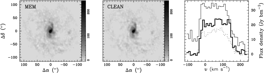
In millimeter interferometry, the relatively low source strengths and relatively high random and systematic errors conspire to ensure that we are almost always working in the low signal-to-noise regime; for BIMA SONG, typical S/N ratios for the channel maps were on the order of 10–40. In BIMA SONG data, we saw the “runaway” flux feature commonly with MEM, where there could be arbitrarily large flux density added into the deconvolved images, depending on what was specified as the convergence criteria. An example of this is shown in Figure 13, which shows BIMA-only maps of integrated intensity for NGC 6946 made using MEM and CLEAN, and spectra of the total flux measured in the inner 200″-diameter region using the different data cubes. As seen in the maps, the flux density in the small-scale components tends to be accurately represented, so that the final MEM and CLEAN images look very similar to one another. But as the spectra show, the low-level flux rides systematically higher with MEM than with CLEAN; in this example, the total flux in the MEM map is over three times higher than that in the CLEAN map. In fact, the total flux density in the BIMA-only MEM map is more than twice the total flux density in the 12m-only map of the same region, which is clearly an unphysical result. In general, the deeper one tries to deconvolve using MEM, the worse the “runaway” flux problem gets. The MEM algorithm performs somewhat better on a linear combination of the BIMA and 12m data, as with the Stanimirovic et al. (1999) method described in Appendix B. In principle, one could fine-tune the convergence criteria for each channel of each map to try to get an accurate flux determination. However, there are pitfalls to doing so: first, if one cuts the deconvolution off too soon, then residual sidelobes might remain in the map; second, specifying the convergence criteria depends on a priori knowledge of the source structure and flux density. In practice it is difficult to fine-tune MEM to work well in the low signal-to-noise regime.
The CLEAN algorithm, first introduced by Högbom (1974), is an iterative procedure that builds a model of the source distribution using an ensemble of point sources. Cornwell, Braun & Briggs (1999) discuss the many variations on the original algorithm contributed by different authors; in BIMA SONG tests, we used the implementation by Steer, Dewdney, & Ito (1984). Since CLEAN does not suffer from the “runaway” flux problem that MEM is subject to, we concluded that it was a far more reliable algorithm to use for accurate flux density representation for BIMA SONG maps; therefore, the maps in this catalog were produced using CLEAN.
While CLEAN does not introduce flux density errors into the map, it also does not produce an ideal deconvolution. As Holdaway & Cornwell (1999) showed, CLEAN does not do as well as MEM at recovering large-scale structure in the map. (These tests were done in the high signal-to-noise regime where MEM does not suffer from the “runaway” flux problem.) This is because the conventional CLEAN source model is inherently built out of point sources, so that it is effectively biased against large-scale (and especially low-level) emission in a map, whereas MEM inherently assumes a large-scale, smooth distribution as a default model.
A problem that is common to conventional CLEAN algorithms as well as to MEM is that both algorithms tend to omit systematically distributed residuals from the source models; the residuals, even if at a level consistent with the 1 noise specification, take the general shape of the source distribution in each channel map (Fig. 14). This feature can introduce a bias for algorithms like self-calibration, which depend on the model to be an accurate representation of the source structure. It can also lead to an inaccurate flux density determination in the final map: the final (“restored”) map is usually made by convolving the source model (i.e. the output from the deconvolution algorithm) with an idealized, gaussian beam, and then adding the derived residuals to the result. The smoothed model map therefore has units of flux density per “clean beam”, whereas the residual map has units of flux density per “dirty beam”. If one is at all fortunate, then the dirty beam has an area that is not too dissimilar to that of the clean beam, so that the convolved model and the residuals are on the same flux scale. But if there is a significant contribution to the total flux density that remains in the residual map, as may occur when there is a broad, low-level source, and if the clean beam and the dirty beam have slightly different areas, then the total flux density in the restored map might again be inaccurately represented. The best one can do to alleviate this problem is to clean as deeply as practical, so that as much of the flux density is represented in the source model as is possible.
To summarize, (1) the CLEAN algorithm is probably a better choice than MEM for imaging sources with S/N ratios 1000, which covers most non-masing sources at millimeter wavelengths with current telescopes. MEM may produce images with the correct peak flux density, but it may also produce images with unphysically high total flux density because of the “runaway” flux problem. (2) It is extremely advantageous to get as much of the source flux density into the deconvolution model as is possible, by cleaning as deeply as is practical. That way, even if the model and the residuals are on different flux density scales, it is only the noise measurement that is ill-defined. The signal-to-noise estimates may then be affected, but the source flux density would be properly represented.
Appendix B Single Dish and Interferometric Data Combination Techniques
While the idea of incorporating single dish data into interferometric data is not new (cf Emerson 1974 for the first combined image – H I in M33, and Vogel et al. 1984 for the first combined mm- image – HCO+ in Orion), the practice is far from routine. The 24 combined BIMA12 m maps presented in this paper comprise by far the largest collection of single dish interferometric maps published to date. However, millimeter astronomers recognize the importance of incorporating single dish data for making accurate maps of large ( 20–30″ at 115 GHz) structures: for the international Atacama Large Millimeter Array (ALMA) that is currently under development, the twin capabilities of mosaicing many fields on the sky and of incorporating single-dish data into interferometric maps together drive some of the most ambitious technical specifications for the antenna design.
Holdaway (1999) has presented an excellent, detailed discussion of techniques of combining mosaiced data with total power data, most of which have been implemented and tested on high S/N data taken at centimeter wavelengths. Indeed, in noise-free simulations by Helfer et al. (2002), we recovered all the flux density in a resolved-out source by simply adding a discrete total power point measured at ()=(0,0) and relying on the deconvolution to do the proper extrapolation between the total power point and the interferometric data. With real millimeter data, problems with pointing offsets and drifts, relative calibration between the telescopes, phase noise and atmospheric decorrelation in the interferometer data, and deformation of the telescope dish and therefore the primary beam, combine to place severe constraints on the deconvolution. With the added difficulty that the signal-to-noise ratios are typically much lower, data combination tends to be much more challenging in the millimeter regime than at centimeter wavelengths.
For BIMA SONG, we tried a variety of data combination techniques to determine what worked best empirically for our data. For many of our tests, it was possible to fine-tune a single spectral channel to achieve seemingly good pointing or calibration agreement, but there would be a fairly random scatter of such solutions across the 20-40 spectral channels that together made up a data cube. We therefore tried to achieve a solution that gave the best results for the data cube as a whole.
B.1 Addition of Short- and Zero-Spacing Data in the Plane
In this technique, first demonstrated on 3 mm spectral line data by Vogel et al. (1984), the single-dish data are sampled at spatial frequencies 0 , where is the diameter of the single dish telescope. In brief, an idealized single-dish primary beam response function is deconvolved from the single-dish OTF maps, to form a model of what the source looks like on the sky. For each of the interferometer pointing centers, a model field is then generated by multiplying the sky model by the idealized interferometer primary beam at that position. The model field is then sampled at chosen points.
In practice, this technique can be fine-tuned to work very well, if one has enough patience. Unfortunately, the exact results tend to depend on the details of the parameters chosen, from the method for the single-dish deconvolution to the distribution, number and weighting of the points specified (which can significantly alter the synthesized beam from the interferometer-only case). As a check, one can model visibilities just in the overlap region of the plane that both the single dish and the interferometer sample and compare the calibration and structures in the resulting maps of the overlap visibilities (e.g. Wilner & Welch, 1994); however, in relatively low S/N observations, this comparison of the overlap region is usually unsatisfactory. In the end, one can gauge the success of the data combination by comparing the final combined map, convolved to the resolution of the single-dish telescope, to the single-dish data alone. If by inspection the agreement is not good, one can go back, adjust the calibration or try a different (deeper or more shallow) single-dish deconvolution, and try again. In summary, while adding single-dish data in the plane can be very successful given enough attention to the combination, it is typically time-consuming and hard to automate.
B.2 Addition of Single-Dish Data in the Image Plane
There are both linear and nonlinear methods of adding the single-dish data to an interferometric map in the image plane. In the linear method (implemented as IMMERGE in MIRIAD), the interferometric data are deconvolved separately. The separate single-dish and interferometer images are each transformed and then merged in the Fourier plane, using a tapering function in the overlap region to specify the weights of each data set. One can check the goodness of fit in the overlap region by comparing the data derived from each of the two input images. However, with the S/N ratios of 10–40 per spectral channel that were typical for BIMA SONG data, the calibration in the overlap region depended rather sensitively on the exact region chosen for the overlap. One also needs to be cautious when a large amount of flux density is resolved out by the interferometer; in this case, the interferometer-only deconvolution may run into difficulties. In practice, Wong (2000) used this technique successfully for CO-rich BIMA SONG galaxies.
Sault, Staveley-Smith, & Brouw (1996) presented a nonlinear joint deconvolution algorithm (implemented as MOSMEM in MIRIAD) that Sault later modified to incorporate single dish data. In this method, a joint maximum entropy deconvolution is performed on a linear mosaic of the “dirty” (undeconvolved) interferometer fields along with the single-dish data; the algorithm maximizes the entropy, subject to two separate constraints from the two data sets. This technique has been applied very successfully for centimeter-wavelength data and for high S/N millimeter-wavelength data (e.g. Welch et al., 2000). However, given the low S/N “runaway” flux problem associated with the maximum entropy deconvolution and described in Appendix A, this method did not turn out to be a successful approach for BIMA SONG data.
Instead, for BIMA SONG, we adopted a linear combination technique described in Stanimirovic et al. (1999). In this method, we created a new “dirty” map by a linear combination of the interferometer map prior to deconvolving and the single dish map, where the single dish map had been weighted by an idealized form of the interferometer’s primary gain of the mosaiced pointings. We scaled the single dish map by the ratio of the area of the interferometer beam to the area of the single dish beam, and created a new “dirty” beam by the same linear combination of the interferometer synthesized beam and the single dish beam (assumed to be a truncated gaussian). We then deconvolved the new combined “dirty” map using a Steer-Dewdney-Ito CLEAN algorithm. This method is easy to implement and automate, with relatively few parameters to specify.
References
- Binney et al. (1991) Binney, J., Gerhard, O. E., Stark, A. A., Bally, J., & Uchida, K. I. 1991, MNRAS, 252, 210
- Binney & Merrifield (1998) Binney, J. & Merrifield, M. 1998, Galactic Astronomy, Princeton, Princeton University Press, 1998
- Blitz (1993) Blitz, L. 1993, Protostars and Planets III, 125
- Blitz (1997) Blitz, L. 1997, IAU Symp. 170: CO: Twenty-Five Years of Millimeter-Wave Spectroscopy, 170, 11
- Braun (1997) Braun, R. 1997, ApJ, 484, 637
- Briggs (1995) Briggs, D. S. 1995, AAS Meeting, 187, 112.02
- Brouillet et al. (1991) Brouillet, N., Baudry, A., Combes, F., Kaufman, M., & Bash, F. 1991, A&A, 242, 35
- Casoli et al. (1998) Casoli, F. et al. 1998, A&A, 331, 451
- Cornwell, Braun & Briggs (1999) Cornwell, T., Braun, R. & Briggs, D. S. 1999, ASP Conf. Ser. 180: Synthesis Imaging in Radio Astronomy II, 151
- Cornwell, Holdaway & Uson (1993) Cornwell, T. J. Holdaway, M. A. & Uson, J. M. 1993, A&A, 271, 697
- Crane, Giuffrida, & Carlson (1976) Crane, P. C., Giuffrida, T. S., & Carlson, J. B. 1976, ApJ, 203, L113
- Crosthwaite, Turner, & Ho (2000) Crosthwaite, L.P., Turner, J.L., & Ho, P.T.P. 2000, AJ, 119, 1720
- Crosthwaite et al. (2001) Crosthwaite, L. P., Turner, J. L., Hurt, R. L., Levine, D. A., Martin, R. N., & Ho, P. T. P. 2001, AJ, 122, 797
- Dame (1993) Dame, T. M. 1993, AIP Conf. Proc. 278: Back to the Galaxy, 267
- de Bruyn, Crane, Price, & Carlson (1976) de Bruyn, A. G., Crane, P. C., Price, R. M., & Carlson, J. B. 1976, A&A, 46, 243
- de Vaucouleurs et al. (1995) de Vaucouleurs, G., de Vaucouleurs, A., Corwin, H. G., Buta, R. J., Paturel, G., & Fouque, P. 1995, VizieR Online Data Catalog, 7155, 0 (RC3)
- Ekers & Rots (1979) Ekers, R. D. & Rots, A. H., 1979, in Image Formation from Coherence Functions in Astronomy, ed. C. van Schooneveld (Dordrecht:Reidel), 61
- Elmegreen & Elmegreen (1987) Elmegreen, D.M. & Elmegreen B.G. 1987, ApJ, 314, 3
- Emerson (1974) Emerson, D. T. 1974, MNRAS, 169, 607
- Emerson & Graeve (1988) Emerson, D. T. & Graeve, R. 1988, A&A, 190, 353
- Emerson (1996) Emerson, D. T. 1996, in IAU symposium 170, ed. W. B. Latter, S. J. E. Radford, P. R. Jewell, J. G. Mangum, & J. Bally (Kluwer), 207
- Engargiola et al. (2002) Engargiola, G., Plambeck, R. L., Rosolowsky, E., & Blitz, L. 2002, in preparation
- Ferrarese et al. (1996) Ferrarese, L. et. al. 1996, ApJ, 464, 568
- Freedman et al. (1994) Freedman, W.L., et al. 1994, ApJ, 427, 628
- Frei et al. (1996) Frei, Z., Guhathakurta, P., Gunn, J.E. & Tyson, J.A. 1996, AJ, 111, 174
- Gibson et al. (1999) Gibson, B.K. 1999, ApJ, 512, 48
- Graham et al. (1997) Graham, J.A. et al. 1997, ApJ, 477, 535
- Graham et al. (1999) Graham, J.A. et al. 1999, ApJ, 516, 626
- Güsten (1989) Güsten, R. 1989, IAU Symp. 136: The Center of the Galaxy, 136, 89
- Helfer & Blitz (1995) Helfer, T. T. & Blitz, L. 1995, ApJ, 450, 90
- Helfer et al. (2002) Helfer, T. T., Vogel, S. N., Lugten, J. B., & Teuben, P. J. 2002, PASP, 114, 350
- Heyer, Dame, & Thaddeus (2000) Heyer, M. H., Dame, T. M., & Thaddeus, P. 2000, The Interstellar Medium in M31 and M33. Proceedings 232. WE-Heraeus Seminar, 22-25 May 2000, Bad Honnef, Germany. Edited by Elly M. Berkhuijsen, Rainer Beck, and Rene A. M. Walterbos. Shaker, Aachen, 2000, p. 29-36, 29
- Ho, Filippenko, & Sargent (1997) Ho, L.C., Filippenko, A.V., & Sargent, W.L.W. 1997, ApJS, 112, 315
- Högbom (1974) Högbom, J. A. 1974, A&AS, 15, 417
- Holdaway (1999) Holdaway, M. A. 1999, ASP Conf. Ser. 180: Synthesis Imaging in Radio Astronomy II, 401
- Holdaway & Cornwell (1999) Holdaway, M. A. & Cornwell, T. J. 1999, URSI meeting, Toronto
- Hughes (1998) Hughes, S. M. et al. 1998, ApJ, 501, 32
- Kelson et al. (1996) Kelson, D.D. 1996, ApJ, 463, 26
- Lay (1999) Lay, O., BIMA Memorandum No. 72
- Loinard et al. (1996) Loinard, L., Dame, T. M., Koper, E., Lequeux, J., Thaddeus, P., & Young, J. S. 1996, ApJ, 469, L101
- Loinard et al. (1999) Loinard, L., Dame, T. M., Heyer, M. H., Lequeux, J., & Thaddeus, P. 1999, A&A, 351, 1087
- Macri et al. (1999) Macri, L.M., et al. 1999, ApJ, 521, 155
- Macri et al. (2001) Macri, L.M., Stetson, P.B., Bothun, G.D., Freedman, W.L., Garnavich, P.M., Jha, S., Madore, B.F., & Richmond, M.W. 2001 , ApJ, 559, 243
- Maoz et al. (1999) Maoz, E., Newman, J. A., Ferrarese, L., Stetson, P. B., Zepf, S. E., Davis, M., Freedman, W.Ł. & Madore, B. F. 1999, Nature, 401, 351
- Möllenhoff & Heidt (2001) Möllenhoff, C. & Heidt, J. 2001,A&A, 368, 16
- Nishiyama & Nakai (2001) Nishiyama, K. & Nakai, N. 2001, PASJ, 53, 713
- Paglione et al. (2001) Paglione, T. A. D. et al. 2001, ApJS, 135, 183
- Regan (2000) Regan, M. W. 2000, ApJ, 541, 142
- Regan & Elmegreen (1997) Regan, M. W. & Elmegreen, D. M. 1997, AJ, 114, 965
- Regan, Sheth, & Vogel (1999) Regan, M. W., Sheth, K., & Vogel, S. N. 1999, ApJ, 526, 97
- Regan et al. (2001) Regan, M.W., Thornley, M.D., Helfer, T.T., Sheth, K., Wong, T., Vogel, S.N., Blitz, L., & Bock, D.C.-J. 2001, ApJ, 561, 218 (Paper I)
- Regan et al. (2002) Regan, M.W., Sheth, K., Teuben, P.J., & Vogel, S.N. 2002, ApJ, 574, 126
- Rickard et al. (1975) Rickard, L. J., Palmer, P., Morris, M., Turner, B. E., & Zuckerman, B. 1975, ApJ, 199, L75
- Saha et al. (1999) Saha A., Sandage, A., Tammann, G. A., Labhardt, L., Macchetto, F. D. & Panagia, N. 1999, ApJ, 522, 802
- Sakamoto et al. (1999) Sakamoto, K., Okumura, S. K., Ishizuki, S., & Scoville, N. Z. 1999, ApJS, 124, 403
- Sandage (1961) Sandage, A. 1961, The Hubble Atlas of Galaxies, Washington: Carnegie Institution, 1961
-
Sault (1999)
Sault, R.J. 1999, MIRIAD User’s Guide,
http://www.atnf.csiro.au/computing/software/miriad/userhtml.html - Sault, Staveley-Smith, & Brouw (1996) Sault, R. J., Staveley-Smith, L., & Brouw, W. N. 1996, A&AS, 120, 375
- Sault, Teuben, & Wright (1995) Sault, R.J., Teuben, P.J., & Wright, M.C.H. 1995, in Astronomical Data Analysis Software and Systems IV, eds. R.A. Shaw, H.E. Payne, & J.J.E. Hayes, A.S.P. Conference Series 77, 433
- Sheth et al. (2002) Sheth, K., Vogel. S. N., Regan, M. W., Teuben, P. J., Harris, A. I., Thornley, M. D., & Helfer, T. T., 2002, submitted to ApJ
- Silbermann et al. (1996) Silbermann, N.A. et al. 1996, ApJ, 470, 1
- Sodroski et al. (1994) Sodroski, T. J. et al. 1994, ApJ, 428, 638
- Stanimirovic et al. (1999) Stanimirovic, S., Staveley-Smith, L., Dickey, J.M., Sault, R.J., & Snowden, S. 1999, MNRAS, 302, 417
- Steer, Dewdney, & Ito (1984) Steer, D. G., Dewdney, P. E., & Ito, M. R. 1984, A&A, 137, 159
- Tanvir, Ferguson, & Shanks (1999) Tanvir, N.R., Ferguson, H.C., & Shanks, T. 1999, MNRAS, 310, 175
- Thornley (1996) Thornley, M. D. 1996, ApJ, 469, L45
- Tully (1988) Tully, R.B. 1988, Nearby Galaxies Catalog (Cambridge University Press: New York)
- Turner et al. (1998) Turner, A. et al. 1998, ApJ, 505, 297
- Verter (1990) Verter, F. 1990, PASP, 102, 1281
- Vogel et al. (1984) Vogel, S. N., Wright, M. C. H., Plambeck, R. L. & Welch, W. J. 1984, ApJ, 283, 655
- Welch et al. (2000) Welch, W. J., Hartmann, L., Helfer, T., & Briceño, C. 2000, ApJ, 540, 362
- Welch et al. (1996) Welch, W. J. et al. 1996, PASP, 108, 93
- Wilner & Welch (1994) Wilner, D.J. & Welch, W.J. 1994, ApJ, 427, 898
- Wong (2000) Wong, T. 2000, Ph.D. Dissertation, University of California at Berkeley
- Wong & Blitz (2000) Wong, T. & Blitz, L. 2000, ApJ, 540, 771
- Wong & Blitz (2002) Wong, T. & Blitz, L. 2002, ApJ, 549, 157
- Young et al. (1995) Young, J. S. et al. 1995, ApJS, 98, 219
- Young & Scoville (1991) Young, J. S. & Scoville, N. Z. 1991, ARA&A, 29, 581
- Zaritsky, Kennicutt, & Huchra (1994) Zaritsky, D., Kennicutt, R. C., & Huchra, J. P. 1994, ApJ, 420, 87
| Source | (J2000)aaAdopted tracking center and LSR velocity of the observations. | (J2000)aaAdopted tracking center and LSR velocity of the observations. | aaAdopted tracking center and LSR velocity of the observations. | PAbbInclination () and position angle (PA) from RC3, except where noted. | RC3 Type | NuclearccSpectral classification from Ho, Filippenko, & Sargent (1997). HII = H II nucleus, Sy = Seyfert nucleus, L = LINER, and T = transition object, which has [O I] strengths intermediate between those of H II nuclei and LINERs. One (:) or two (::) colons following the classification signifies uncertain and highly uncertain classifications. | Distance | Arm ClassddArm class (AC) from Elmegreen & Elmegreen (1987). AC 1–4 are flocculents, and AC 5–12 are grand design spirals. | ||||
|---|---|---|---|---|---|---|---|---|---|---|---|---|
| ( ) | (° ′ ″) | (km s-1) | (°) | (°) | Classification | (Mpc) | Reference | (′) | mag | |||
| NGC 0628 | 01 36 41.7 | 15 46 59 | 657 | 24eeFrom Paper I. | 25eeFrom Paper I. | SA(s)c | 7.3 | 1 | 10.5 | 9.95 | 9 | |
| NGC 0925 | 02 27 16.9 | 33 34 45 | 553 | 56 | 102 | SAB(s)d | HII | 9.29 | 2 | 10.5 | 10.69 | 1 |
| NGC 1068 | 02 42 40.7 | 00 00 48 | 1136 | 33eeFrom Paper I. | 13eeFrom Paper I. | (R)SA(rs)b | Sy1.8 | 14.4 | 1 | 7.1 | 9.61 | 3 |
| IC 342 | 03 46 49.7 | 68 05 45 | 34 | 31ffFrom kinematic fitting, Crosthwaite, Turner, & Ho (2000). | 37ffFrom kinematic fitting, Crosthwaite, Turner, & Ho (2000). | SAB(rs)cd | HII | 3.9 | 1 | 21.4 | 9.10 | 9 |
| NGC 2403 | 07 36 54.5 | 65 35 58 | 131 | 56 | 127 | SAB(s)cd | HII | 4.2 | 1 | 21.9 | 8.93 | 3 |
| NGC 2841 | 09 22 02.7 | 50 58 36 | 638 | 64 | 147 | SA(r)b: | L2 | 14.1 | 3 | 8.1 | 10.09 | 3 |
| NGC 2903 | 09 32 10.1 | 21 30 02 | 556 | 61eeFrom Paper I. | 17eeFrom Paper I. | SAB(rs)bc | HII | 6.3 | 1 | 12.6 | 9.68 | 7 |
| NGC 2976 | 09 47 17.1 | 67 54 51 | 3 | 63 | 143 | SAc-pec | HII | 2.1 | 1 | 5.9 | 10.82 | 3 |
| NGC 3031 | 09 55 33.2 | 69 03 55 | 34 | 58 | 157 | SA(s)ab | Sy1.5 | 3.63 | 4 | 26.9 | 7.89 | 12 |
| NGC 3184 | 10 18 16.7 | 41 25 27 | 592 | 21 | 135 | SAB(rs)cd | HII | 8.7 | 1 | 7.4 | 10.36 | 9 |
| NGC 3344 | 10 43 31.1 | 24 55 21 | 586 | 24ggFrom optical photometry, Frei et al. (1996). | 0ggFrom optical photometry, Frei et al. (1996). | (R)SAB(r)bc | HII | 6.1 | 1 | 7.1 | 10.45 | 9 |
| NGC 3351 | 10 43 58.0 | 11 42 14 | 778 | 40eeFrom Paper I. | 13eeFrom Paper I. | SB(r)b | HII | 10.1 | 5 | 7.4 | 10.53 | 6 |
| NGC 3368 | 10 46 45.6 | 11 49 18 | 897 | 46ggFrom optical photometry, Frei et al. (1996). | 5ggFrom optical photometry, Frei et al. (1996). | SAB(rs)ab | L2 | 11.2 | 6 | 7.6 | 10.11 | 8 |
| NGC 3521 | 11 05 49.3 | 00 02 02 | 805 | 58eeFrom Paper I. | 164eeFrom Paper I. | SAB(rs)bc | HII/L2:: | 7.2 | 1 | 11.0 | 9.83 | 3 |
| NGC 3627 | 11 20 15.1 | 12 59 22 | 727 | 63eeFrom Paper I. | 176eeFrom Paper I. | SAB(s)b | T2/Sy2 | 11.1 | 7 | 9.1 | 9.65 | 7 |
| NGC 3726 | 11 33 20.7 | 47 01 41 | 849 | 46 | 10 | SAB(r)c | HII | 17.0 | 1 | 6.2 | 10.91 | 5 |
| NGC 3938 | 11 52 49.6 | 44 07 14 | 809 | 24ggFrom optical photometry, Frei et al. (1996). | 0ggFrom optical photometry, Frei et al. (1996). | SA(s)c | HII:: | 17.0 | 1 | 5.4 | 10.90 | 9 |
| NGC 3953 | 11 53 49.0 | 52 19 37 | 1054 | 60 | 13 | SB(r)bc | T2 | 17.0 | 1 | 6.9 | 10.84 | 9 |
| NGC 3992 | 11 57 36.1 | 53 22 29 | 1048 | 52 | 68 | SB(rs)bc | T2: | 17.0 | 1 | 7.6 | 10.60 | 9 |
| NGC 4051 | 12 03 09.6 | 44 31 53 | 725 | 41 | 135 | SAB(rs)bc | Sy1.2 | 17.0 | 1 | 5.2 | 10.83 | 5 |
| NGC 4258 | 12 18 57.5 | 47 18 14 | 448 | 65eeFrom Paper I. | 176eeFrom Paper I. | SAB(s)bc | Sy1.9 | 8.1 | 8 | 18.6 | 9.10 | |
| NGC 4303 | 12 21 54.9 | 04 28 25 | 1566 | 27ggFrom optical photometry, Frei et al. (1996). | 0ggFrom optical photometry, Frei et al. (1996). | SAB(rs)bc | HII | 15.2 | 1 | 6.5 | 10.18 | 9 |
| NGC 4321 | 12 22 54.8 | 15 49 20 | 1571 | 32eeFrom Paper I. | 154eeFrom Paper I. | SAB(s)bc | T2 | 16.1 | 9 | 7.4 | 10.05 | 12 |
| NGC 4414 | 12 26 27.2 | 31 13 24 | 716 | 55eeFrom Paper I. | 159eeFrom Paper I. | SA(rs)c? | T2: | 19.1 | 10 | 3.6 | 10.96 | 3 |
| NGC 4450 | 12 28 29.3 | 17 05 07 | 1954 | 41 | 175 | SA(s)ab | L1.9 | 16.8 | 1 | 5.2 | 10.90 | 12 |
| NGC 4490 | 12 30 36.9 | 41 38 23 | 565 | 60 | 125 | SB(s)d pec | HII | 7.8 | 1 | 6.3 | 10.22 | 1 |
| NGC 4535 | 12 34 20.3 | 08 11 54 | 1961 | 45 | 28hhFrom near-infrared photometry, Möllenhoff & Heidt (2001). | SAB(s)c | HII | 16.0 | 11 | 7.1 | 10.59 | 9 |
| NGC 4548 | 12 35 26.4 | 14 29 49 | 486 | 37 | 150 | SB(rs)b | L2 | 15.9 | 12 | 5.4 | 10.96 | 5 |
| NGC 4559 | 12 35 57.8 | 27 57 36 | 815 | 66 | 150 | SAB(rs)cd | HII | 9.7 | 1 | 10.7 | 10.46 | |
| NGC 4569 | 12 36 49.80 | 13 09 46 | 235 | 62 | 23 | SAB(rs)ab | T2 | 16.8 | 1 | 9.5 | 10.26 | 5 |
| NGC 4579 | 12 37 43.53 | 11 49 05 | 1519 | 37 | 95 | SAB(rs)b | Sy1.9/L1.9 | 16.8 | 1 | 5.9 | 10.48 | 9 |
| NGC 4699 | 12 49 02.33 | 08 39 55 | 1427 | 47 | 45 | SAB(rs)b | 25.7 | 1 | 3.8 | 10.41 | 3 | |
| NGC 4725 | 12 50 26.60 | 25 30 06 | 1206 | 45 | 35 | SAB(r)ab pec | Sy2: | 12.6 | 13 | 10.7 | 10.11 | 6 |
| NGC 4736 | 12 50 53.06 | 41 07 14 | 308 | 35eeFrom Paper I. | 100eeFrom Paper I. | (R)SA(r)ab | L2 | 4.3 | 1 | 11.2 | 8.99 | 3 |
| NGC 4826 | 12 56 44.24 | 21 41 05 | 408 | 54eeFrom Paper I. | 111eeFrom Paper I. | (R)SA(rs)ab | T2 | 4.1 | 1 | 10.0 | 9.36 | 6 |
| NGC 5005 | 13 10 56.23 | 37 03 33 | 946 | 61 | 65 | SAB(rs)bc | L1.9 | 21.3 | 1 | 5.8 | 10.61 | 3 |
| NGC 5033 | 13 13 27.53 | 36 35 38 | 875 | 62 | 170 | SA(s)c | Sy1.5 | 18.7 | 1 | 10.7 | 10.75 | 9 |
| NGC 5055 | 13 15 49.25 | 42 01 49 | 504 | 55 | 105 | SA(rs)bc | T2 | 7.2 | 1 | 12.6 | 9.31 | 3 |
| NGC 5194 | 13 29 52.35 | 47 11 54 | 463 | 15eeFrom Paper I. | 0eeFrom Paper I. | SA(s)bc pec | Sy2 | 7.7 | 1 | 11.2 | 8.96 | 12 |
| NGC 5248 | 13 37 32.06 | 08 53 07 | 1153 | 43 | 110 | SAB(rs)bc | HII | 22.7 | 1 | 6.2 | 10.97 | 12 |
| NGC 5247 | 13 38 02.62 | 17 53 02 | 1357 | 29 | 20 | SA(s)bc | 22.2 | 1 | 5.6 | 10.5 | 9 | |
| NGC 5457 | 14 03 12.48 | 54 20 55 | 241 | 27iiFrom kinematic fitting, Braun (1997). | 40iiFrom kinematic fitting, Braun (1997). | SAB(rs)cd | 7.4 | 14 | 28.8 | 8.31 | 9 | |
| NGC 6946 | 20 34 52.33 | 60 09 14 | 48 | 54eeFrom Paper I. | 65eeFrom Paper I. | SAB(rs)cd | HII | 5.5 | 1 | 11.5 | 9.61 | 9 |
| NGC 7331 | 22 37 04.09 | 34 24 56 | 821 | 62eeFrom Paper I. | 172eeFrom Paper I. | SA(s)b | T2 | 15.1 | 15 | 10.5 | 10.35 | 3 |
References. — (1) Tully (1988);(2) Silbermann et al. (1996); (3) Macri et al. (2001); (4) Freedman et al. (1994); (5) Graham et al. (1997); (6) Tanvir, Ferguson, & Shanks (1999); (7) Saha et al. (1999); (8) Maoz et al. (1999); (9) Ferrarese et al. (1996); (10) Turner et al. (1998); (11) Macri et al. (1999); (12) Graham et al. (1999); (13) Gibson et al. (1999); (14) Kelson et al. (1996); (15) Hughes (1998)
| Source | NfieldsaaNumber of fields observed with the interferometer. | bbFWHM of major and minor axes of synthesized beam. | ccLinear dimensions of major and minor axes of synthesized beam, given the distances in Table 1. | ddBeam position angle. | eeVelocity binning of the channel maps. | ffRms noise level of the channel map, measured over a 120″ 120″ box in emission-free channels in the data cube. Where the velocity binning was other than 10 km s-1, the rms was normalized to that of a 10 km s-1 channel. | Cont. fluxggContinuum flux levels. Upper limits are 3 measurements. For the detections, formal uncertainties are listed; the systematic error is 1 = 15%. | ContourhhStarting contour for the maps of integrated intensity in §5. | iiRms noise level of single-dish OTF channel maps, per 10 km s-1 channel. Where present, this indicates that single-dish OTF maps from the NRAO 12 m telescope were incorporated into the BIMA SONG maps. |
|---|---|---|---|---|---|---|---|---|---|
| (″ ″) | (pc pc) | (°) | (km s-1) | (mJy bm-1) | (Jy bm-1) | (Jy bm-1 km s-1) | (Jy bm-1) | ||
| NGC 0628 | 13 | 7.2 5.3 | 250 190 | 8 | 5 | 51 | 0.012 | 1.5 | 0.69 |
| NGC 0925 | 7 | 6.1 5.6 | 280 250 | 4 | 10 | 65 | 0.013 | 2.5 | |
| NGC 1068 | 13 | 8.9 5.6 | 620 390 | 16 | 10 | 85 | 0.041 0.007 | 6.0 | 0.56 |
| IC 342 | 7 | 5.6 5.1 | 110 97 | 34 | 10 | 129 | 0.027 | 6.0 | 1.47 |
| NGC 2403 | 7 | 6.3 5.8 | 130 120 | 22 | 10 | 49 | 0.009 | 2.0 | |
| NGC 2841 | 7 | 6.1 5.1 | 420 350 | 25 | 20 | 66 | 0.013 | 2.5 | |
| NGC 2903 | 7 | 6.8 5.5 | 210 170 | 9 | 10 | 68 | 0.016 | 5.0 | 0.38 |
| NGC 2976 | 1 | 7.8 6.9 | 79 70 | 59 | 10 | 41 | 0.010 | 1.5 | |
| NGC 3031 | 7 | 5.9 5.1 | 100 90 | 14 | 20 | 58 | 0.161 0.006 | 3.0 | |
| NGC 3184 | 7 | 5.9 5.4 | 250 230 | 12 | 10 | 50 | 0.010 | 1.5 | |
| NGC 3344 | 7 | 6.4 5.3 | 190 160 | 9 | 10 | 50 | 0.011 | 1.3 | |
| NGC 3351 | 7 | 7.4 5.2 | 360 250 | 7 | 10 | 64 | 0.014 | 3.0 | 0.33 |
| NGC 3368 | 7 | 7.7 5.7 | 420 310 | 5 | 10 | 69 | 0.013 | 2.0 | |
| NGC 3521 | 7 | 8.8 5.7 | 310 200 | 1 | 10 | 78 | 0.020 | 5.0 | 0.56 |
| NGC 3627 | 14 | 7.3 5.8 | 390 310 | 80 | 10 | 41 | 0.009 | 5.0 | 0.43 |
| NGC 3726 | 1 | 6.0 5.0 | 500 420 | 11 | 10 | 32 | 0.008 | 1.5 | |
| NGC 3938 | 7 | 5.9 5.4 | 480 440 | 33 | 10 | 59 | 0.014 | 2.5 | 0.31 |
| NGC 3953 | 7 | 6.9 5.8 | 570 480 | 2 | 10 | 72 | 0.015 | 2.0 | |
| NGC 3992 | 7 | 6.6 5.3 | 550 440 | 1 | 10 | 60 | 0.013 | 1.5 | |
| NGC 4051 | 1 | 7.0 4.9 | 580 410 | 2 | 10 | 23 | 0.006 | 1.5 | |
| NGC 4258 | 7 | 6.1 5.4 | 240 210 | 4 | 10 | 60 | 0.013 | 4.0 | 0.26 |
| NGC 4303 | 7 | 7.3 5.5 | 540 400 | 4 | 10 | 47 | 0.011 | 4.0 | 0.66 |
| NGC 4321 | 7 | 7.2 4.9 | 560 380 | 9 | 10 | 50 | 0.014 | 3.0 | 0.94 |
| NGC 4414 | 1 | 6.4 5.0 | 590 460 | 6 | 10 | 29 | 0.008 | 3.0 | 0.36 |
| NGC 4450 | 1 | 6.6 5.1 | 540 410 | 5 | 10 | 43 | 0.013 | 1.5 | |
| NGC 4490 | 1 | 6.0 5.7 | 230 210 | 58 | 10 | 26 | 0.007 | 0.8 | |
| NGC 4535 | 7 | 7.3 5.7 | 570 440 | 2 | 10 | 63 | 0.015 | 2.0 | |
| NGC 4548 | 1 | 7.1 6.2 | 550 480 | 23 | 10 | 43 | 0.011 | 2.0 | |
| NGC 4559 | 7 | 5.9 5.6 | 280 260 | 16 | 10 | 55 | 0.013 | 2.0 | |
| NGC 4569 | 7 | 6.6 5.5 | 540 450 | 2 | 10 | 54 | 0.012 | 3.0 | 0.24 |
| NGC 4579 | 7 | 8.1 7.1 | 660 580 | 11 | 10 | 68 | 0.028 0.006 | 3.5 | |
| NGC 4699 | 1 | 10.3 6.8 | 1300 850 | 11 | 10 | 86 | 0.019 | 3.0 | |
| NGC 4725 | 7 | 7.0 5.4 | 430 330 | 9 | 20 | 86 | 0.017 | 3.0 | |
| NGC 4736 | 7 | 6.9 5.0 | 140 100 | 63 | 10 | 64 | 0.017 | 3.0 | 0.38 |
| NGC 4826 | 7 | 7.5 5.2 | 150 100 | 3 | 10 | 82 | 0.016 | 4.0 | 0.39 |
| NGC 5005 | 1 | 6.2 6.0 | 640 620 | 23 | 10 | 32 | 0.009 | 1.5 | 0.16 |
| NGC 5033 | 7 | 6.1 5.4 | 550 490 | 86 | 20 | 73 | 0.015 | 4.0 | 0.44 |
| NGC 5055 | 7 | 5.8 5.5 | 200 190 | 18 | 10 | 55 | 0.011 | 5.0 | 0.45 |
| NGC 5194 | 26 | 5.8 5.1 | 220 190 | 4 | 10 | 61 | 0.012 | 5.0 | 0.55 |
| NGC 5248 | 1 | 6.9 5.8 | 760 630 | 1 | 10 | 38 | 0.011 | 1.0 | 0.35 |
| NGC 5247 | 1 | 12.2 4.7 | 1300 510 | 2 | 10 | 59 | 0.016 | 3.0 | 0.32 |
| NGC 5457 | 7 | 5.7 5.4 | 210 190 | 59 | 10 | 45 | 0.010 | 3.0 | 0.59 |
| NGC 6946 | 7 | 6.0 4.9 | 160 130 | 14 | 10 | 61 | 0.013 | 6.0 | 0.63 |
| NGC 7331 | 7 | 6.1 4.9 | 440 360 | 5 | 10 | 50 | 0.010 | 3.0 | 0.51 |
| Source | aaLocation of spectra. Offsets are measured from tracking center listed in Table 1. | aaLocation of spectra. Offsets are measured from tracking center listed in Table 1. | bbMeasured rms noise per 2 MHz (5.2 km s-1) channel. | ccIntegrated intensity = , measured over the velocity limits given. The formal uncertainty in the integrated intensity is also tabulated. The systematic uncertainty has an assigned value of about 25% times the integrated intensity; see §3.2.2. For nondetections, a 3 upper limit is given. | ddVelocity limits of integration. | Flux FractioneeRatio of flux recovered in the BIMA spectra, smoothed to 55″, relative to the 12m flux. The formal uncertainty in the ratio is listed. Given the assigned systematic uncertainties of 15% in the BIMA data and 25% in the 12 m data, the systematic uncertainty in the ratio is 30% times the ratio. The ratios are enclosed in parentheses when they are detected at 2 confidence level. See §8.3. |
|---|---|---|---|---|---|---|
| (″) | (″) | (K) | (K km s-1) | (km s-1) | Recovered | |
| NGC 0925 | 0 | 0 | 0.005 | 1.10 0.15 | 495,640 | (0.07 0.38) |
| 22 | 38 | 0.009 | 0.87 | 453,653 | ||
| 44 | 0 | 0.013 | 0.76 0.23 | 480,540 | ||
| 22 | -38 | 0.005 | 1.25 0.14 | 430,550 | (0.06 0.30) | |
| -22 | -38 | 0.006 | 0.57 | 453,653 | ||
| -44 | 0 | 0.012 | 1.1 | 453,653 | ||
| -22 | 38 | 0.007 | 0.69 | 453,653 | ||
| NGC 2403 | 0 | 0 | 0.018 | 2.16 0.29 | 100,200 | 0.63 0.16 |
| 22 | 38 | 0.023 | 1.5 | 31,231 | ||
| 44 | 0 | 0.019 | 1.71 0.25 | 145,210 | (0.19 0.15) | |
| 22 | -38 | 0.017 | 1.14 0.27 | 100,200 | (0.55 0.29) | |
| -22 | -38 | 0.015 | 1.46 0.25 | 90,200 | 0.56 0.23 | |
| -44 | 0 | 0.020 | 1.4 | 31,231 | ||
| -22 | 38 | 0.020 | 1.95 0.39 | 50,200 | (0.24 0.18) | |
| NGC 2841 | 0 | 0 | 0.008 | 1.4 | 290,930 | |
| 22 | 38 | 0.010 | 1.7 | 290,930 | ||
| 44 | 0 | 0.010 | 1.7 | 290,930 | ||
| 22 | -38 | 0.011 | 1.9 | 290,930 | ||
| -22 | -38 | 0.009 | 1.7 | 290,930 | ||
| -44 | 0 | 0.011 | 1.8 | 290,930 | ||
| -22 | 38 | 0.010 | 1.8 | 290,930 | ||
| NGC 2976 | 0 | 0 | 0.007 | 1.29 0.15 | -35,45 | (0.49 0.42) |
| NGC 3031 | 0 | 0 | 0.013 | 1.3 | -134,66 | |
| 22 | 38 | 0.021 | 2.0 | -134,66 | ||
| 44 | 0 | 0.014 | 1.3 | -134,66 | ||
| 22 | -38 | 0.014 | 1.4 | -134,66 | ||
| -22 | -38 | 0.020 | 1.9 | -134,66 | ||
| -44 | 0 | 0.015 | 1.5 | -134,66 | ||
| -22 | 38 | 0.011 | 1.25 0.28 | 70,180 | ||
| NGC 3184 | 0 | 0 | 0.004 | 3.96 0.09 | 550,660 | 0.54 0.07 |
| 22 | 38 | 0.008 | 3.10 0.17 | 535,620 | 0.28 0.08 | |
| 44 | 0 | 0.007 | 2.44 0.14 | 560,635 | 0.30 0.10 | |
| 22 | -38 | 0.008 | 2.79 0.17 | 550,645 | (0.17 0.09) | |
| -22 | -38 | 0.007 | 2.43 0.14 | 570,650 | (0.16 0.10) | |
| -44 | 0 | 0.009 | 2.72 0.22 | 510,630 | (0.05 0.10) | |
| -22 | 38 | 0.010 | 2.35 0.24 | 500,600 | (0.07 0.11) | |
| NGC 3344 | 0 | 0 | 0.015 | 3.28 0.45 | 475,650 | (0.01 0.11) |
| 22 | 38 | 0.018 | 2.85 0.53 | 490,660 | ||
| 44 | 0 | 0.016 | 1.1 | 500,600 | ||
| 22 | -38 | 0.014 | 1.90 0.22 | 500,545 | (0.02 0.10) | |
| -22 | -38 | 0.019 | 3.34 0.46 | 500,610 | (0.06 0.08) | |
| -44 | 0 | 0.010 | 2.25 0.30 | 475,650 | (0.13 0.15) | |
| -22 | 38 | 0.013 | 2.28 0.24 | 600,660 | 0.19 0.09 | |
| NGC 3368 | 0 | 0 | 0.006 | 12.80 0.32 | 670,1200 | 0.94 0.06 |
| 22 | 38 | 0.009 | 0.90 | 797,997 | ||
| 44 | 0 | 0.007 | 3.04 0.29 | 800,1100 | 0.36 0.17 | |
| 22 | -38 | 0.007 | 3.32 0.28 | 800,1100 | 0.73 0.16 | |
| -22 | -38 | 0.007 | 4.23 0.30 | 750,1100 | 0.28 0.13 | |
| -44 | 0 | 0.008 | 3.54 0.32 | 680,1000 | (0.27 0.15) | |
| -22 | 38 | 0.007 | 4.58 0.27 | 680,1000 | 0.26 0.11 | |
| NGC 3726 | 0 | 0 | 0.010 | 2.88 0.33 | 760,960 | (0.43 0.25) |
| NGC 3953 | 0 | 0 | 0.010 | 4.57 0.39 | 860,1170 | (0.10 0.16) |
| 22 | 38 | 0.009 | 4.90 0.32 | 1030,1250 | (0.06 0.13) | |
| 44 | 0 | 0.011 | 3.09 0.41 | 950,1200 | (0.06 0.22) | |
| 22 | -38 | 0.009 | 3.99 0.30 | 870,1100 | (0.05 0.16) | |
| -22 | -38 | 0.009 | 4.71 0.25 | 850,1000 | (0.13 0.11) | |
| -44 | 0 | 0.010 | 5.21 0.43 | 840,1170 | (0.05 0.15) | |
| -22 | 38 | 0.009 | 5.62 0.33 | 1000,1240 | (0.06 0.12) | |
| NGC 3992 | 0 | 0 | 0.008 | 1.0 | 800,1200 | |
| 22 | 38 | 0.008 | 1.1 | 800,1200 | ||
| 44 | 0 | 0.007 | 1.54 0.21 | 800,950 | (-0.22 0.22) | |
| 22 | -38 | 0.009 | 1.3 | 800,1200 | ||
| -22 | -38 | 0.008 | 1.1 | 800,1200 | ||
| -44 | 0 | 0.010 | 1.54 0.45 | 800,1200 | ||
| -22 | 38 | 0.009 | 2.06 0.43 | 800,1200 | ||
| NGC 4051 | 0 | 0 | 0.012 | 8.68 0.42 | 615,845 | 0.34 0.06 |
| NGC 4450 | 0 | 0 | 0.011 | 4.17 0.46 | 1800,2150 | (0.18 0.32) |
| NGC 4490 | 0 | 0 | 0.004 | 1.63 0.12 | 550,720 | (0.27 0.34) |
| NGC 4535 | 0 | 0 | 0.011 | 8.26 0.45 | 1810,2120 | 0.65 0.07 |
| 22 | 38 | 0.020 | 3.99 0.56 | 1810,1960 | 0.29 0.10 | |
| 44 | 0 | 0.019 | 5.12 0.64 | 1860,2090 | 0.31 0.09 | |
| 22 | -38 | 0.019 | 3.83 0.49 | 1950,2080 | 0.21 0.09 | |
| -22 | -38 | 0.018 | 3.86 0.49 | 1950,2095 | 0.31 0.10 | |
| -44 | 0 | 0.024 | 2.09 0.61 | 1915,2040 | 0.41 0.20 | |
| -22 | 38 | 0.019 | 3.17 0.50 | 1810,1945 | 0.31 0.12 | |
| NGC 4548 | 0 | 0 | 0.005 | 2.77 0.19 | 305,625 | (0.31 0.42) |
| NGC 4559 | 0 | 0 | 0.008 | 3.09 0.26 | 715,910 | 0.31 0.12 |
| 22 | 38 | 0.012 | 1.1 | 715,910 | ||
| 44 | 0 | 0.011 | 1.0 | 715,910 | ||
| 22 | -38 | 0.011 | 1.99 0.28 | 690,825 | (0.26 0.16) | |
| -22 | -38 | 0.008 | 0.78 | 715,910 | ||
| -44 | 0 | 0.011 | 1.97 0.30 | 750,900 | (-0.04 0.16) | |
| -22 | 38 | 0.009 | 1.80 0.23 | 790,910 | (0.22 0.17) | |
| NGC 4579 | 0 | 0 | 0.006 | 6.33 0.26 | 1310,1705 | 0.32 0.08 |
| 22 | 38 | 0.014 | 3.73 0.62 | 1310,1705 | (0.17 0.14) | |
| 44 | 0 | 0.013 | 2.56 0.36 | 1565,1705 | (0.13 0.12) | |
| 22 | -38 | 0.014 | 2.09 0.36 | 1525,1645 | ||
| -22 | -38 | 0.015 | 5.62 0.49 | 1320,1540 | (0.13 0.07) | |
| -44 | 0 | 0.019 | 3.89 0.66 | 1320,1540 | ||
| -22 | 38 | 0.020 | 3.71 0.67 | 1320,1540 | ||
| NGC 4699 | 0 | 0 | 0.011 | 1.5 | 1250,1620 | |
| NGC 4725 | 0 | 0 | 0.007 | 2.80 0.32 | 1030,1400 | (0.60 0.31) |
| 22 | 38 | 0.010 | 1.3 | 1030,1400 | ||
| 44 | 0 | 0.018 | 2.3 | 1030,1400 | ||
| 22 | -38 | 0.015 | 1.9 | 1030,1400 | ||
| -22 | -38 | 0.015 | 1.9 | 1030,1400 | ||
| -44 | 0 | 0.012 | 1.5 | 1030,1400 | ||
| -22 | 38 |
| Source | aaAngular length of square region over which flux density is measured. | bbGlobal flux densities measured over square region of length . See Figure 6 for flux densities as a function of varying . | ccCO luminosities, or 4 , where is the distance to the galaxy, listed in Table 1. | ddCO mass enclosed within region measured. = 7845 , where is in Mpc, the CO/H2 conversion factor is assumed to be 2 1020 cm-2 (K km s-1)-1, and no correction for heavy elements is made. | |
|---|---|---|---|---|---|
| (′) | (Jy km s-1) | (106 Jy km s-1 Mpc2) | (109 M☉) | ||
| NGC 0628 | 6 | 0.57 | 1514 63eeFormal uncertainties are listed; the systematic error is 1 = 15%. | 1.01 0.04eeFormal uncertainties are listed; the systematic error is 1 = 15%. | 0.63 0.03eeFormal uncertainties are listed; the systematic error is 1 = 15%. |
| NGC 1068 | 6 | 0.85 | 4102 217 | 10.69 0.57 | 6.67 0.35 |
| IC 342 | 6 | 0.28 | 9847ffSize of emitting region is much larger than 6′ for IC 342; this flux density should not be interpreted as a global flux measurement. 418 | 1.88ffSize of emitting region is much larger than 6′ for IC 342; this flux density should not be interpreted as a global flux measurement. 0.08 | 1.17ffSize of emitting region is much larger than 6′ for IC 342; this flux density should not be interpreted as a global flux measurement. 0.05 |
| NGC 2903 | 6 | 0.48 | 3254 282 | 1.62 0.14 | 1.01 0.09 |
| NGC 3351 | 6 | 0.81 | 1513 221 | 1.94 0.28 | 1.21 0.18 |
| NGC 3521 | 6 | 0.55 | 4800 353 | 3.13 0.23 | 1.95 0.14 |
| NGC 3627 | 6 | 0.66 | 4259 427 | 6.59 0.66 | 4.12 0.41 |
| NGC 3938 | 5 | 0.93 | 923 73 | 3.35 0.27 | 2.09 0.17 |
| NGC 4258 | 6 | 0.32 | 2686 255 | 2.21 0.21 | 1.38 0.13 |
| NGC 4303 | 6 | 0.92 | 2427 145 | 7.05 0.42 | 4.40 0.26 |
| NGC 4321 | 6 | 0.81 | 2972 319 | 9.68 1.04 | 6.04 0.65 |
| NGC 4414 | 6 | 1.67 | 2453 282 | 11.25 1.29 | 7.02 0.81 |
| NGC 4569 | 6 | 0.63 | 1096 137 | 3.89 0.49 | 2.43 0.30 |
| NGC 4736 | 6 | 0.54 | 2641 155 | 0.39 0.05 | 0.24 0.03 |
| NGC 4826 | 6 | 0.60 | 1845 217 | 0.61 0.04 | 0.38 0.02 |
| NGC 5005 | 6 | 1.03 | 1278 484 | 7.29 2.76 | 4.55 1.72 |
| NGC 5033 | 5 | 0.47 | 2469 258 | 10.85 1.13 | 6.77 0.71 |
| NGC 5055 | 6 | 0.48 | 3812 276 | 2.48 0.18 | 1.55 0.11 |
| NGC 5194 | 12ggRegion for NGC 5194 is a rectangle with lengths . | 1.07 | 10097 267 | 7.52 0.20 | 4.70 0.12 |
| NGC 5248 | 6 | 0.97 | 1829 195 | 11.84 1.26 | 7.39 0.79 |
| NGC 5247 | 5 | 0.89 | 1102 91 | 6.82 0.56 | 4.26 0.35 |
| NGC 5457 | 7 | 0.24 | 3479 265 | 2.39 0.18 | 1.49 0.11 |
| NGC 6946 | 6 | 0.52 | 9273 241 | 3.52 0.09 | 2.20 0.06 |
| NGC 7331 | 6 | 0.57 | 2762 367 | 7.91 1.05 | 4.94 0.66 |
| Source | aaPeak face-on molecular surface brightness in the galaxy. | bbCentral face-on molecular surface brightness, measured at the highest position in the central 6″. Central positions taken from Sheth et al. (2002). | / |
|---|---|---|---|
| (M☉ pc-2) | (M☉ pc-2) | ||
| NGC 0628 | 104 | 20 | 0.20 |
| NGC 0925 | 31 | 0 | 0.00 |
| NGC 1068 | 947 | 466 | 0.49 |
| IC 342 | 1267 | 1151 | 0.91 |
| NGC 2403 | 30 | 25 | 0.81 |
| NGC 2841 | 36 | 0 | 0.00 |
| NGC 2903 | 573 | 573 | 1.00 |
| NGC 2976 | 15 | 15 | 1.00 |
| NGC 3031 | 24 | 0 | 0.00 |
| NGC 3184 | 153 | 153 | 1.00 |
| NGC 3344 | 24 | 0 | 0.00 |
| NGC 3351 | 426 | 406 | 0.95 |
| NGC 3368 | 815 | 645 | 0.79 |
| NGC 3521 | 103 | 82 | 0.80 |
| NGC 3627 | 539 | 539 | 1.00 |
| NGC 3726 | 94 | 94 | 1.00 |
| NGC 3938 | 72 | 60 | 0.82 |
| NGC 3953 | 23 | 0 | 0.00 |
| NGC 3992 | 18 | 5 | 0.32 |
| NGC 4051 | 315 | 315 | 1.00 |
| NGC 4258 | 473 | 202 | 0.43 |
| NGC 4303 | 432 | 432 | 1.00 |
| NGC 4321 | 442 | 442 | 1.00 |
| NGC 4414 | 130 | 59 | 0.46 |
| NGC 4450 | 15 | 10 | 0.71 |
| NGC 4490 | 18 | 0 | 0.00 |
| NGC 4535 | 429 | 429 | 1.00 |
| NGC 4548 | 18 | 18 | 1.00 |
| NGC 4559 | 16 | 13 | 0.80 |
| NGC 4569 | 510 | 510 | 1.00 |
| NGC 4579 | 99 | 89 | 0.90 |
| NGC 4699 | 15 | 5 | 0.34 |
| NGC 4725 | 69 | 21 | 0.32 |
| NGC 4736 | 327 | 327 | 1.00 |
| NGC 4826 | 672 | 672 | 1.00 |
| NGC 5005 | 724 | 724 | 1.00 |
| NGC 5033 | 188 | 188 | 1.00 |
| NGC 5055 | 335 | 328 | 0.98 |
| NGC 5194 | 787 | 216 | 0.28 |
| NGC 5248 | 344 | 323 | 0.94 |
| NGC 5247 | 108 | 108 | 1.00 |
| NGC 5457 | 348 | 348 | 1.00 |
| NGC 6946 | 1854 | 1854 | 1.00 |
| NGC 7331 | 164 | 31 | 0.19 |