Linear Polarization in Gamma-Ray Bursts: The Case for an Ordered Magnetic Field

Abstract

Linear polarization at the level of $\sim 1-3\%$ has by now been measured in several GRB afterglows. Whereas the degree of polarization, $P$, was found to vary in some sources, the position angle, $\theta_{p}$, was roughly constant in all cases. Until now, the polarization has been commonly attributed to synchrotron radiation from a jet with a tangled magnetic field that is viewed somewhat off axis. However, this model predicts either a peak in $P$ or a $90^{\circ}$ change in $\theta_{p}$ around the “jet break” time in the lightcurve, for which there has so far been no observational confirmation. We propose an alternative interpretation, wherein the polarization is attributed, at least in part, to a large-scale, ordered magnetic field in the ambient medium. The ordered component may dominate the polarization even if the total emissivity is dominated by a tangled field generated by postshock turbulence. In this picture, $\theta_{p}$ is roughly constant because of the uniformity of the field, whereas $P$ varies as a result of changes in the ratio of the ordered-to-random mean-squared field amplitudes. We point out that variable afterglow light curves should be accompanied by a variable polarization. The radiation from the original ejecta, which includes the prompt $\gamma$-ray emission and the emission from the reverse shock (the ‘optical flash’ and ‘radio flare’), could potentially exhibit a high degree of polarization (up to $\sim 60\%$) induced by an ordered transverse magnetic field advected from the central source.

1. Introduction

The first detection of polarization in an optical afterglow was in GRB 990510, where a degree of polarization $P=1.7\pm 0.2\%$ ($1.6\pm 0.2\%$) was measured at $t_{\rm obs}\approx 18\;$hr ($21\;$hr) after the burst. Since then, $P\sim 1-3\%$ has been detected in a few additional afterglows, some of which showed a temporal variation in $P$ (Rol et al. 2000; Barth et al. 2003), but typically the position angle (PA) $\theta_{p}$ showed little or no change. A few other afterglows produced only upper limits, $P\lesssim 2-5\%$.

The polarization is attributed to synchrotron emission behind a shock wave. It thus depends on the local magnetic field configuration, which determines the polarization at each point of the afterglow image, and on the global geometry of the shock, which determines how the polarization is averaged over the (unresolved) image. We make a distinction between magnetic field configurations that are axially symmetric about the normal $\hat{n}_{\rm sh}$ to the shock surface and those that are not. The first category gives no net polarization for a spherical flow and is assumed in most previous works (Sari 1999; Ghisellini & Lazzati 1999; Medvedev & Loeb 1999; Granot et al. 2002; Rossi et al. 2002). These models take the field to be completely random in the plane of the shock, and the polarization is usually attributed to a jet viewed somewhat off axis. For a structured jet, $P$ has one peak near the jet break time $t_{j}$ (when $1/\gamma$ increases to $\sim\theta_{0}$, the initial jet opening half-angle), whereas for a uniform jet $P$ has 2 (or 3) peaks near $t_{j}$, with $P$ passing through zero and $\theta_{p}$ changing by $90^{\circ}$ between the peaks.

The second category can produce net polarization even for a spherical flow. One example is the “patchy coherent field” model of Gruzinov & Waxman (1999), where the observed region consists of $N\sim 50$ mutually incoherent patches of angular size $\lesssim 1/\gamma$, within each of which the field is fully ordered. This model predicts $P\sim P_{\rm max}/N^{1/2}\sim 10\%$ (where $P_{\rm max}\sim 60-70\%$ is the maximum $P$ of local synchrotron emission in a uniform magnetic field) and simultaneous (random) variability in $P$ and $\theta_{p}$ on timescales $\Delta t_{\rm obs}\lesssim t_{\rm obs}$ . The idea behind this model is that $\sim 1/\gamma$ is the angular size of causally connected regions, and for a magnetic field that is generated in the shock itself this is the largest scale over which the field can be coherent.

However, if the magnetic field were ordered on an angular scale $\theta_{B}\gtrsim 1/\gamma$, then the resulting $P$ could approach $P_{\rm max}$. Such a situation can be realized if an ordered field exists in the medium into which the shock propagates. For a typical interstellar medium, the postshock field would still be very weak (with the magnetic energy a fraction $\epsilon_{B}\lesssim 10^{-10}$ of the internal energy), but it would be higher ($\epsilon_{B}\lesssim 10^{-4}$; Biermann & Cassinelli 1993) if the shock expands into a magnetized wind of a progenitor star, and higher yet ($\epsilon_{B}\sim 0.01-0.1$) if it propagates into a pulsar-wind bubble (PWB), as expected in the supranova model (Königl & Granot 2002). A strong ordered field component is likely to exist in the original ejecta and could give rise to a high value of $P$ ($\lesssim P_{\rm max}$) in both the prompt GRB and the reverse-shock emission.

We calculate the polarization for a jet with a tangled magnetic field in § 2, investigate the effects of adding an ordered field component in § 3, and discuss the results in § 4.

2. Polarization from a Jet with a Tangled Magnetic Field

Synchrotron emission is generally partially linearly polarized. In terms of the Stokes parameters: $V\equiv 0$, $\theta_{p}=\frac{1}{2}\arctan(U/Q)$, and $P=(Q^{2}+U^{2})^{1/2}/I$. As the Stokes parameters are additive for incoherent emission, they can be calculated by summing over all the contributions from different fluid elements to the flux at a given observed time $t_{\rm obs}$. In practice, the flux is calculated by dividing $t_{\rm obs}$ into bins of size $\delta t_{\rm obs}$, and assigning to the appropriate time bin the contribution to $F_{\nu}$ from the emission of each 4-volume fluid element $d^{4}x$,

$$dF_{\nu}(t_{\rm obs},\hat{n},{\bf r},t)={(1+z)^{2}\over d_{L}^{2}}{\,j^{\prime}_{\nu^{\prime}}({\bf r},t)\Theta(\delta t_{\rm obs}-2|t-\frac{\hat{n}\cdot{\bf r}}{c}-t_{\rm obs}|)d^{4}x\over\gamma^{2}({\bf r},t)\left[1-\hat{n}\cdot{\bf v}({\bf r},t)/c\right]^{2}\delta t_{\rm obs}}\ ,$$ (1)

$$\left\{\begin{matrix}U/I\vspace{0.12cm}\cr Q/I\end{matrix}\right\}=\left(\sum dF_{\nu}\right)^{-1}\sum dF_{\nu}\left\{\begin{matrix}P\sin 2\theta_{p}\vspace{0.12cm}\cr P\cos 2\theta_{p}\end{matrix}\right\}\ ,$$ (2)

where $j^{\prime}_{\nu^{\prime}}$ is the local emissivity, ${\bf v}$ is the fluid velocity, $\hat{n}$ is the direction to the observer, $\Theta$ is the Heaviside step function and the summation in Eq. 2 is over ${\bf r}$ & $t$, for fixed $t_{\rm obs}$ & $\hat{n}$.

In this section, we consider only a random magnetic field $B_{\rm rnd}$ that is tangled on angular scales $\ll 1/\gamma$, with axial symmetry w.r.t. $\hat{n}_{\rm sh}$. The field anisotropy is parameterized by $b\equiv 2\langle B_{\parallel}^{2}\rangle/\langle B_{\perp}^{2}\rangle$, where $B_{\parallel}$ ($B_{\perp}$) is the magnetic field component parallel (perpendicular) to $\hat{n}_{\rm sh}$. The local polarization of the emission from a given fluid element is

$${P_{\rm rnd}(\theta^{\prime})\over P_{\rm max}}={\left(\langle B_{\parallel}^{2}\rangle-\langle B_{\perp}^{2}\rangle/2\right)\sin^{2}\theta^{\prime}\over\langle B_{\parallel}^{2}\rangle\sin^{2}\theta^{\prime}+(1+\cos^{2}\theta^{\prime})\langle B_{\perp}^{2}\rangle/2}={(b-1)\sin^{2}\theta^{\prime}\over 2+(b-1)\sin^{2}\theta^{\prime}}\ ,$$ (3)

(Gruzinov 1999; Sari 1999), where $\cos\theta^{\prime}=\frac{\mu-v/c}{1-\mu v/c}$, $\mu\equiv\hat{n}\cdot\hat{n}_{\rm sh}$. For $P>0$, the polarization is in the direction of $\hat{n}\times\hat{n}_{\rm sh}$.

The magnetic field configuration behind the shock, and hence the value of $b$, cannot be easily deduced from first principles. It was suggested that small-scale postshock fields can be generated by a two-stream instability (e.g., Medvedev & Loeb 1999), which predicts $b\ll 1$. However, it is not clear whether the magnetic fields produced in this way survive in the bulk of the postshock flow (Gruzinov 1999, although see Frederiksen et al. 2003), or whether this is the dominant tangling mechanism. The relatively low observed values of $P$ ($\lesssim 3-4\%$) suggest that $0.5\lesssim b\lesssim 2$ if the polarization is due to a jet with a shock-generated field.

Turbulence in the postshock region (possibly induced by a microinstability) could amplify and isotropize the field, keeping $b$ close to $1$. As each fluid element moves downstream from the shock transition, it is sheared by the flow. For a Blandford-McKee (1976) self-similar blastwave solution with an ambient density $\rho_{\rm ext}\propto r^{-k}$, the length of a fluid element in the directions parallel and perpendicular to $\hat{n}_{\rm sh}$ scales with the self-similarity variable $\chi$ (where $\chi=1$ at the shock front and increases with distance behind the shock) as $L_{\parallel}\propto\chi^{\frac{9-2k}{2(4-k)}}$ and $L_{\perp}\propto\chi^{\frac{1}{4-k}}$. Therefore, the stretching of each fluid element in the radial direction is larger than in the tangential direction. This would increase $b$ while maintaining axial symmetry about $\hat{n}_{\rm sh}$. The relevant value of $b$ here is the average over the postshock region, weighted by the emissivity. If the turbulence only persists over a small distance ($0<\chi-1\ll 1$, but still $\gg$ the plasma skin depth) then, since most of the emission is from $\chi\lesssim$ a few, we may have $1<b\lesssim\;$a few.

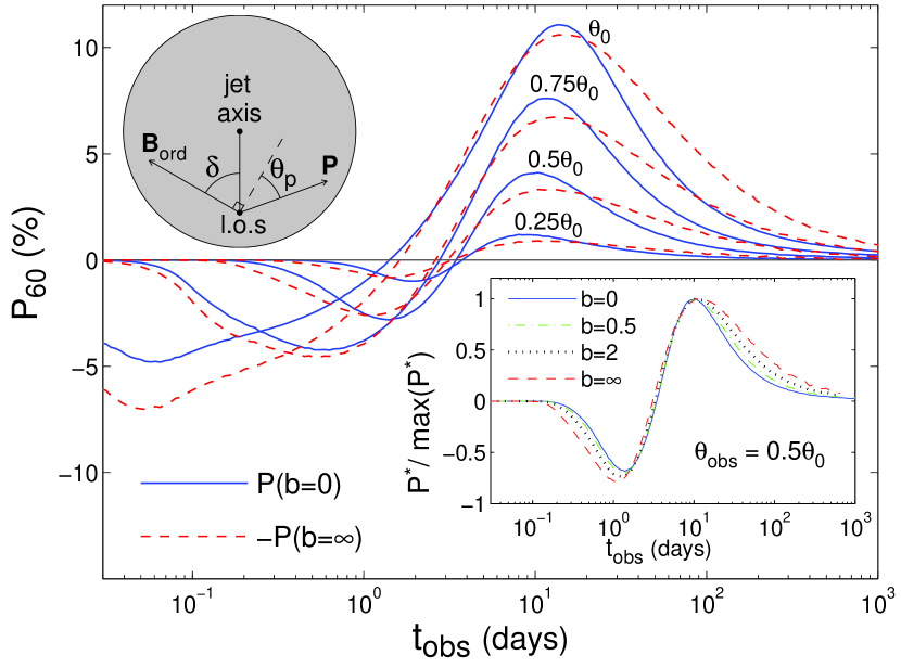
Figure 1.— Polarization lightcurves for a jetted GRB afterglow with a random magnetic field. The solid (dashed) lines are for $b=0$ ($b=\infty$, with a minus sign); $P_{60}\equiv P(0.6/P_{\rm max})$. The jet parameters are the same as in Fig. 3 of Granot et al. (2002). The lower right inset shows $P^{*}\equiv{\rm sgn}(1-b)P$, normalized to its maximum value, for a viewing angle $\theta_{\rm obs}=0.5\,\theta_{0}$ and $b=0,0.5,2,\infty$, making it easier to follow the effect of $b$ on the shape of the lightcurve. The upper left inset shows a schematic diagram of the plane of the sky. The shaded region represents a jet with both a tangled and ordered field components. The projection of the ordered magnetic field on the plane of the sky, ${\bf B}_{\rm ord}$, is at an angle $\delta$ in the counterclockwise direction w.r.t. the direction from the line of sight (l.o.s.) to the jet axis. The polarization vector ${\bf P}$ is at an angle $\theta_{p}$, measured clockwise from the perpendicular to ${\bf B}_{\rm ord}$.

Figure 1 shows the polarization lightcurves for $b=0$ and $\infty$, based on the jet model of Kumar & Panaitescu (2000). For all viewing angles $\theta_{\rm obs}\leq\theta_{0}$ there are two peaks in $P$, a little before and after $t_{j}$: $P$ passes through zero in between these peaks as $\theta_{p}$ changes by $90^{\circ}$. This result is similar to that of Ghisellini & Lazzati (1999), who did not consider lateral spreading of the jet, and differs from that of Sari (1999), who assumed $\theta_{\rm jet}(t_{\rm obs}$$>$$t_{j})=1/\gamma$, since the lateral spreading in the jet model that we use is smaller than the one used by Sari. The main distinction between the $b<1$ and $b>1$ cases is a $90^{\circ}$ difference in $\theta_{p}$, but this prediction can only be tested if one can independently determine the direction from the l.o.s. to the jet axis. This may in principle be done by measuring the direction of motion of the flux centroid $\hat{n}_{c}$ (Sari 1999): for $b<1$, $\hat{P}$ is perpendicular to (aligned with) $\hat{n}_{c}$ before (after) $t_{j}$, whereas for $b>1$ the situation is reversed. More generally, one would then be able to test if indeed $\hat{P}\parallel\hat{n}_{c}$ or $\hat{P}\perp\hat{n}_{c}$, as expected for a pure $B_{\rm rnd}$ field, or if the angle between them is different, as would generally be the case if an ordered field component were also present.

3. The Effects of an Ordered Magnetic Field

We now add an ordered magnetic field component $B_{\rm ord}$ to the random field $B_{\rm rnd}$ considered in § 2. In passing through the shock transition, the parallel component of the ambient magnetic field $B_{\rm ext}$ remains unchanged but the transverse component is amplified by a factor equal to the fluid compression ratio, which for $\gamma\gg 1$ is $4\gamma$. Thus typically $B_{\perp}\gg B_{\parallel}$ behind the shock. For simplicity we assume that $B_{\rm ord}$ lies in the plane of the shock and is fully ordered and that $B_{\rm ext}$ is uniform, so that $B_{\rm ord}$ is coherent over the entire shock.

It is most convenient to sum over the Stokes parameters associated with $B_{\rm rnd}$ and $B_{\rm ord}$ separately and combine them at the end. The direction of polarization $\hat{P}_{\rm ord}$ of the emission from the ordered component is perpendicular to its projection (${\bf B}_{\rm ord}$) on the plane of the sky; $\hat{P}_{\rm rnd}$ is either along the plane containing the l.o.s. and the jet symmetry axis (for $P_{\rm rnd}>0$) or perpendicular to that direction (for $P_{\rm rnd}<0$). The total polarization and the PA are given by

$$P = \left({\eta P_{\rm ord}\over 1+\eta}\right)\left[1+\left({P_{\rm rnd}\over\eta P_{\rm ord}}\right)^{2}-2\left({P_{\rm rnd}\over\eta P_{\rm ord}}\right)\cos 2\delta\right]^{1/2}\ ,$$ (4)

$$\theta_{p} = {1\over 2}\arctan\left({\sin 2\delta\over\cos 2\delta-\eta P_{\rm ord}/P_{\rm rnd}}\right)\ ,$$ (5)

where $\eta\equiv I_{\rm ord}/I_{\rm rnd}\approx\langle B_{\rm ord}^{2}\rangle/\langle B_{\rm rnd}^{2}\rangle$ is the ratio of the observed intensities in the two components and $\theta_{p}\,,\,\delta$ are measured as illustrated in the upper left inset of Figure 1.

For $B_{\rm ord}$ we find that the PA as a function of the polar angle $\theta$ from the l.o.s. and the azimuthal angle $\phi$ (measured from $\hat{B}_{\rm ord}$) is given, in the relativistic ($\gamma\gg 1$) limit, by $\theta_{p}=\phi+\arctan(\frac{1-y}{1+y}\cot\phi)$, where $y\equiv(\gamma\theta)^{2}$. We have $I_{\nu}=I^{\prime}_{\nu^{\prime}}(\nu/\nu^{\prime})^{3}$, with $I^{\prime}_{\nu^{\prime}}\propto\nu^{\prime-\alpha}[1-(\hat{n}^{\prime}\cdot\hat{B}^{\prime}_{\rm ord})^{2}]^{\epsilon/2}$, where $\nu/\nu^{\prime}\approx\frac{2\gamma}{1+y}$ and $1-(\hat{n}^{\prime}\cdot\hat{B}^{\prime}_{\rm ord})^{2}\approx\left(\frac{1-y}{1+y}\right)^{2}\cos^{2}\phi+\sin^{2}\phi$. The Stokes parameters are given by $(U,Q)/IP_{\rm max}=\int d\Omega I_{\nu}(\sin 2\theta_{p},\cos 2\theta_{p})/\int d\Omega I_{\nu}$. For a spherical flow or a jet at $t<t_{j}$, when the edge of the jet is not visible, $\int d\Omega=\int_{0}^{2\pi}d\phi\int_{0}^{y_{\rm max}}dy$, $U=0$ and $\theta_{p}=\pi/2$. For $\epsilon=2$ and $y_{\rm max}=1$ we obtain $-Q/IP_{\rm max}\equiv f(\alpha)=\frac{(2^{4+\alpha}-1)(2+\alpha)(3+\alpha)}{2^{7+\alpha}-28+2\alpha[2^{3+\alpha}5-7+(2^{3+\alpha}-1)\alpha]}$, so $P_{\rm ord}/P_{\rm max}=f(\alpha)\approx 0.90-0.93$ for $0<\alpha<1.5$. For $\alpha=\frac{p-1}{2}$, $P_{\rm max}=\frac{p+1}{p+7/3}$, $\epsilon=\frac{p+1}{2}$ (i.e. PLS G in Granot & Sari 2002), our analytic result corresponds to $p=3$, for which $P_{\rm ord}/P_{\rm max}=\frac{93}{101}\approx 0.92$ and $P_{\rm ord}=\frac{279}{404}\approx 0.69$. For $y_{\rm max}\gg 1$, $\epsilon=2$ we obtain $f(\alpha)=\frac{(2+\alpha)(3+\alpha)}{8+5\alpha+\alpha^{2}}$; for $\alpha=\frac{p-1}{2}$ and $p=3$, $P_{\rm ord}/P_{\rm max}=\frac{6}{7}\approx 0.86$ and $P=\frac{9}{14}\approx 0.64$. The diference between the $y_{\rm max}=1$ and $y_{\rm max}\gg 1$ results may be relevant to the prompt GRB (see § 4), where the tail of a pulse (which corresponds to $y>1$) is predicted to be less polarized than its peak ($y\lesssim 1$). When the edge of the jet is visible, the limits of integration over $d\Omega$ change. As this causes relatively small modifications in $\theta_{p}$ and $P_{\rm ord}$, we use the analytic expressions above for simplicity.

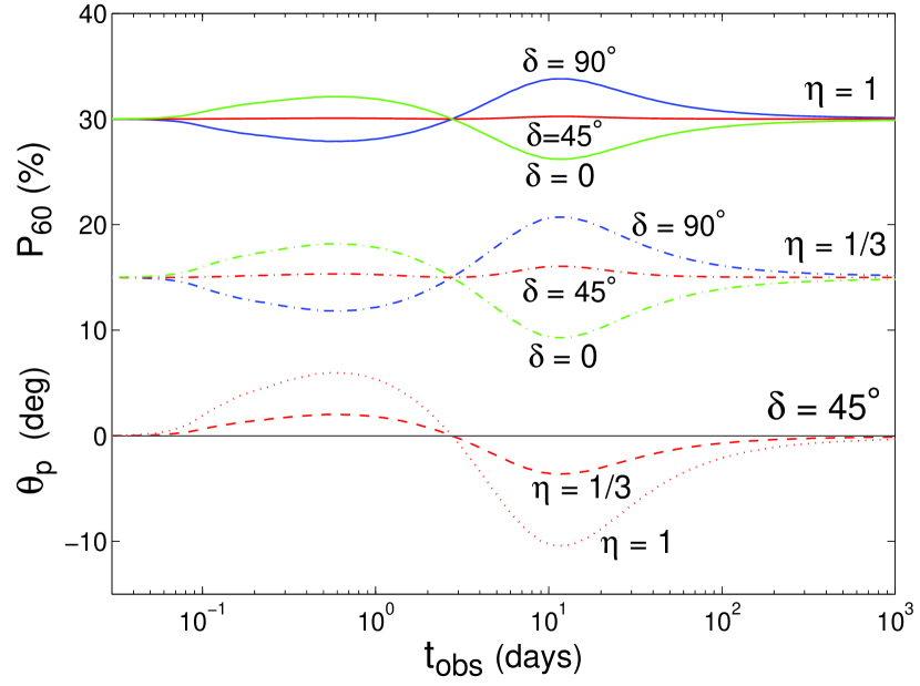
Figure 2.— Polarization lightcurves for ordered $+$ random magnetic field components, for $b=0$ and the same jet parameters as in Fig. 1. As $\theta_{p}(\delta=0,90^{\circ})\equiv 0$, we show only $\theta_{p}(t,\delta=45^{\circ})$.

Figure 2 depicts a sample of polarization lightcurves in which both $\eta$ and $b$ are taken to be independent of time. In this case the $B_{\rm ord}$-induced polarization is constant (in both $P$ and $\theta_{p}$) throughout the afterglow. Interestingly, a similar polarization signature could be produced by dust in our galaxy or in the GRB host galaxy. In the latter case, however, the polarization would likely be accompanied by absorption that would redden the spectrum: this could in principle make it possible to estimate the level of the galactic dust contribution and thereby determine the fraction of such a constant-polarization component that is intrinsic to the source. Since $P_{\rm ord}\approx P_{\rm max}$ whereas $P_{\rm rnd}$ is typically much smaller, we find that for $\eta=1$, and even for $\eta=1/3$, the polarized intensity is still dominated by $B_{\rm ord}$ ($\eta P_{\rm ord}>P_{\rm rnd}$), with $B_{\rm rnd}$ only inducing relatively small fluctuations around the $B_{\rm ord}$-induced values of $P$ and $\theta_{p}$. For $\delta=45^{\circ}$ the fluctuations in both $P$ and $\theta_{p}$ are very small in this parameter range.

If $B_{\rm ord}$ dominates the polarization, then, by equation (4), the time evolution of $P$ follows that of the intensity ratio $\eta$. The low measured values of $P$ indicate that $\eta\ll 1$, so $B_{\rm rnd}$ dominates the emissivity. To the extent that the random field is close to equipartition ($\epsilon_{B,{\rm rnd}}\sim 1$), $\eta=\epsilon_{B,{\rm ord}}/\epsilon_{B,{\rm rnd}}\sim\epsilon_{B,{\rm ord}}$. If the shock is radiative during its early evolution, then cooling-induced compression increases the emissivity-weighted $\epsilon_{B,{\rm ord}}$ over its immediate postshock (adiabatic) value by a factor $\sim(1-\epsilon_{e})^{-1}$. The transition from fast to slow cooling, which occurs at $t=t_{0}$, could therefore reduce $\eta$ and may contribute to the early decline of $P$ observed in some sources. During the subsequent, slow-cooling phase, $\epsilon_{B,{\rm ord}}$ is essentially equal to the magnetization parameter of the ambient medium, $\sigma=B_{\rm ext}^{2}/4\pi\rho_{\rm ext}c^{2}$, so the evolution of $P$ during that phase may reflect the radial behavior of this parameter: $\sigma$ is expected to be roughly constant for an ISM or a stellar wind but to increase with $r$ inside a PWB (Königl & Granot 2002). If the orientation of the ambient field also changed with radius then this would lead to a gradual variation in $\theta_{p}$. If one approximates $B_{\rm ext}\propto r^{a/2}$ and $\rho_{\rm ext}\propto r^{-k}$, then $\epsilon_{B,{\rm ord}}\propto t_{\rm obs}^{\frac{a+k}{4-k}}$. We parameterize the above effects by $\epsilon_{B,{\rm ord}}=\epsilon_{B,0}(t_{\rm obs}/t_{0})^{\frac{a+k}{4-k}}F(t_{\rm obs}/t_{0})$, where $F(x)=1+\frac{g-1}{g+1}\frac{2}{\pi}\arctan(\xi\ln x)$ describes the amplitude ($g$) and sharpness ($\xi$) of the change in $\epsilon_{B,{\rm ord}}$ at $t_{\rm obs}\sim t_{0}$. We assume that $\epsilon_{B,{\rm tot}}=\epsilon_{B,{\rm ord}}+\epsilon_{B,{\rm rnd}}={\rm const}$, so $\eta=(\frac{\epsilon_{B,{\rm tot}}}{\epsilon_{B,{\rm ord}}}-1)^{-1}$.

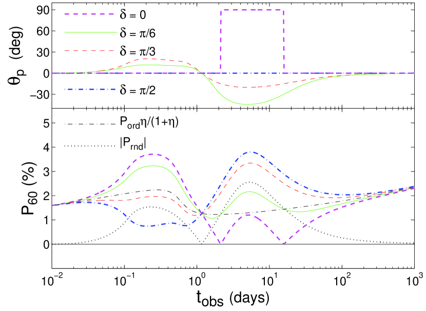
Figure 3.— Polarization lightcurves for a jet with $\theta_{0}=3^{\circ}$, $\theta_{\rm obs}=0.75\theta_{0}$, $b=0.5$, $\epsilon_{B,{\rm tot}}=0.05$, $\epsilon_{e}=0.1$, $t_{j}\approx t_{0}=14\;{\rm hr}$, and $\eta(t)$ given by $\epsilon_{B,0}=0.0015$, $a=2$, $k=0$, $g=3$, and $\xi=3$.

Figure 3 shows an example of the polarization lightcurves. The choice of parameters for $\eta(t)$ is motivated by GRB 020813, in which $\theta_{p}$ was again roughly constant with time whereas $P$ first decreased (from $P\approx 2\%$ after $\sim 6\,{\rm hr}$ to $P\approx 0.6\%$ after $\sim 24\,{\rm hr}$) and subsequently increased monotonically, reaching $P\approx 3.7\%$ after $96\,{\rm hr}$. A sharp break in the lightcurve was observed after $14\;{\rm hr}$ (Covino et al. 2003b). It is seen that roughly equal contributions to the polarization from $B_{\rm ord}$ and $B_{\rm rnd}$ can provide a qualitative fit to the evolution of $P$ and $\theta_{p}$ in this source for $\delta\approx 60^{\circ}-90^{\circ}$. More generally, the polarization lightcurves can show a diverse behavior that varies as a function of $\delta$ as well as of $b$ and $\theta_{\rm obs}/\theta_{0}$. So long as $\eta P_{\rm ord}>P_{\rm rnd}$, the changes in $\theta_{p}$ would be small whereas the variations in $P$ could be significant, as found observationally.

4. Discussion

The linear polarization in GRB afterglows may be largely due to an ordered magnetic field in the ambient medium, which gives rise to an ordered field component behind the afterglow shock that is coherent over the entire emission region. This can result in a polarization position angle (PA), $\theta_{p}$, that is roughly constant in time as well as in a variable degree of polarization, $P$, as found in all afterglow observations to date (except one; see footnote 11).

The magnetic field in the GRB ejecta is potentially much more ordered than in the shocked ambient medium behind the afterglow shock, reflecting the likely presence of a dynamically important, predominantly tansverse, large-scale field advected from the source (e.g., Spruit, Daigne, & Drenkhahn 2001; Vlahakis & Königl 2001). This could result in a large value of $P$ [up to $\sim(0.90-0.93)P_{\rm max}\sim 60\%$] in the prompt $\gamma$-ray emission as well as in the ‘optical flash’ and ‘radio flare’, which are attributed to emission from the reverse shock. If the polarization from the reverse shock is indeed dominated by the ordered component, and if it is coherent over the whole ejecta, then $\theta_{p}$ is not expected to vary significantly during the optical flash or between the optical flash and the radio flare. However, if the ordered magnetic field is coherent only in patches of angular size $\theta_{B}$, then, so long as $\gamma>1/\theta_{B}$, we expect $P\sim P_{\rm max}$, whereas after $\gamma$ drops below $1/\theta_{B}$ we expect $P\sim\gamma\theta_{B}P_{\rm max}$ and variations in $\theta_{p}$ on timescales $\Delta t_{\rm obs}\lesssim t_{\rm obs}$ on account of the averaging over $N\sim(\gamma\theta_{B})^{-2}$ mutually incoherent patches within the observed region of angle $1/\gamma$ about the line of sight. (This resembles the proposal by Gruzinov & Waxman 1999, except that here $N$ is envisioned to increase with time.) In the latter case $P$ might be smaller and $\theta_{p}$ would be different in the ‘radio flare’ (for which typically $\gamma\lesssim 10$) than in the ‘optical flash’ (for which $\gamma\gtrsim 100$).

Variability in the afterglow lightcurve, as reported in GRBs 021004 and 030329, whether induced by a clumpy external medium or a patchy shell (Lazzati et al. 2002; Nakar, Piran, & Granot 2002), should give a different weight to emission from different parts of the afterglow image, thus breaking its symmetry and inducing polarization. Therefore, we expect a highly variable lightcurve to be accompanied by variability in both $P$ and $\theta_{p}$.

Early polarization measurements, starting at $t_{\rm obs}\ll t_{j}$, are crucial for distinguishing between our model and purely tangled jet field models, as the latter predict $P(t_{\rm obs}\ll t_{j})\ll P(t_{\rm obs}\sim t_{j})$, whereas our model allows $P(t_{\rm obs}\ll t_{j})\sim P(t_{\rm obs}\sim t_{j})$. In the latter models $P$ is expected to peak, or else vanish and reappear rotated by $90^{\circ}$, around $t_{j}$. In contrast, in our model, if the polarization is dominated by an ordered magnetic field, then the variations in the polarization around $t_{j}$ would be much less pronounced, with $\theta_{p}$ exhibiting only a gradual variation and $P$ never crossing zero. Our model predicts a possible change in $P$ around the transition time from fast to slow cooling, $t_{0}$, where typically $t_{0}\sim 1\;$hr ($\sim 1\;$day) for ISM-like (stellar wind-like) parameters (although it may vary considerably around these values).

References

- Barth et al. (2003) Barth, A. J., et al. 2003, ApJ, 584, L47
- Bersier et al. (2003) Bersier, D., et al. 2003, ApJ, 583, L63
- Biermann & Cassinelli (1993) Biermann, P. I., & Cassinelli, J. P. 1993, A&A, 277, 691
- Blandford & McKee (1976) Blandford, R. D., & McKee, C. F. 1976, Phys. Fluids, 19, 1130
- Coburn & Boggs (2003) Coburn, W., & Boggs, S.E. 2003, Nature, 423, 415
- Covino et al. (2003a) Covino, S., Ghisellini, G., Lazzati, D., & Malesani, D. 2003a, in GRBs in the Afterglow Era — 3rd Workshop, in press (astro-ph/0301608)
- Covino et al. (2003b) Covino, S., et al. 2003b, A&A, 404, L5
- Frederiksen et al. (2003) Frederiksen, J. T., et al. 2003, preprint (astro-ph/0303360)
- Ghisellini & Lazzati (1999) Ghisellini, G., & Lazzati, D. 1999, MNRAS, 309, L7
- Granot (2003) Granot, J. 2003, ApJL in press (astro-ph/0306322)
- Granot & Königl (2001) Granot, J., & Königl, A. 2001, ApJ, 560, 145
- Granot & Sari (2002) Granot, J., & Sari, R. 2002, ApJ, 568, 820
- Granot et al. (2002) Granot, J., Panaitescu, A., Kumar, P., & Woosley, S. E. 2002, ApJ, 570, L61
- Gruzinov (1999) Gruzinov, A. 1999, ApJ, 525, L29
- Gruzinov & Waxman (1999) Gruzinov, A. & Waxman, E. 1999, ApJ, 511, 852
- Königl & Granot (2002) Königl, A., & Granot, J. 2002, ApJ, 574, 134
- Kumar & Panaitescu (2000) Kumar, P, & Panaitescu, A. 2000, ApJ, 541, L9
- Lazzati et al. (2002) Lazzati, D., et al. 2002, A&A, 396, L5
- Loeb & Perna (1998) Loeb, A., & Perna, R. 1998, 495, 597
- Medvedev & Loeb (1999) Medvedev, M. V., & Loeb, A. 1999, ApJ, 526, 697
- Nakar, Piran & Granot (2003) Nakar, E., Piran, T., & Granot, J. 2003, New Astr., 8, 495
- Rol et al. (2000) Rol, E., et al. 2000, ApJ, 544, 707
- Rol et al. (2003) Rol, E., et al. 2003, A&A Letters, in press (astro-ph/0305227)
- Rossi et al. (2002) Rossi, E., et al. 2002, preprint (astro-ph/0211020)
- Sari (1999) Sari, R. 1999, ApJ, 524, L43
- Spruit, Daigne, & Drenkhahn (2001) Spruit, H. C., Daigne, F., & Drenkhahn, G. 2001, A&A, 369, 694
- Vlahakis & Königl (2001) Vlahakis, N., & Königl, A. 2001, ApJ, 563, L129