The First Heroic Decade of Microlensing

Abstract

We describe the fundamentals of vanilla and exotic microlensing. Deviations from the standard form of an achromatic, time-symmetric lightcurve can be caused by the parallax and xallarap effects, finite source sized effects and binarity. Three applications of microlensing from the First Heroic Decade are reviewed in detail – namely (i) searches for compact dark objects in the Galactic halo, (ii) probes of the baryonic mass distribution in the inner Galaxy and the Andromeda Galaxy and (iii) studies of the limb darkening of source stars. Finally, we suggest four projects for the Second Heroic Decade – (i) K band microlensing towards the Bulge, (ii) pixel lensing towards the low luminosity spiral galaxy M33, (iii) polarimetry of on-going microlensing events and (iv) astrometric microlensing with the GAIA satellite.

Institute of Astronomy, Madingley Rd, Cambridge, CB3 0HA, UK

1. Introduction

This is the end of the First Heroic Decade of Gravitational Microlensing. The pioneering experiments of MACHO, EROS and OGLE reported first candidate events exactly ten years ago (Alcock et al. 1993; Aubourg et al. 1993; Udalski et al. 1993). This led to a frenzied outburst of activity that is only just now beginning to subside. After a decade of glorious achievement, two of the original collaborations (MACHO and EROS) are winding up. Now is an opportune moment to summarise the achievements of the First Heroic Decade, as well as to speculate on what is needed to make the forthcoming decade just as grand!

Historically, the discovery of microlensing at high optical depth predates that of microlensing at low optical depth. The first-ever event that was recognised as microlensing was the bump in the lightcurve of image A of the Einstein Cross (Irwin et al. 1989; Corrigan et al. 1991). The importance of microlensing at low optical depth was generally realised only after a visionary publication of Paczyński’s (1986), in which the idea of monitoring stellar images in the Large Magellanic Cloud was first convincingly mooted. At outset, the impetus for the microlensing surveys was the dark matter problem. Many compact dark matter candidates in the Galactic halo would betray their presence through microlensing. The great achievement of MACHO and EROS has been to rule out most forms of compact dark matter as the dominant contributors to the dark halo. The richness of the microlensing phenomenon has led to applications above and beyond the original aims of the surveys. These include probes of galactic structure and stellar populations, delineation of the Galactic bar, studies of limb darkening and planet searching. The next decade will surely see these applications centre-stage.

2. The Fundamentals

2.1. Vanilla Microlensing

Figure 1.: The source (S), lens (L) and observer (O) are all aligned, so the observer sees a bright Einstein ring of radius $R_{\rm E}$. Its size projected onto the observer’s plane is ${\tilde{R}}_{\rm E}$ and onto the source plane is ${\hat{R}}_{\rm E}$.

Figure 2.: The source (S), lens (L) and observer (O) are now misaligned, so the observer sees two micro-images, one of which is depicted here. (The second micro-image lies on the other side of the lens).

Suppose photons impinge upon a nearby mass $M$ with impact parameter $b$. Then, the General Theory of Relativity predicts that the photons are deflected through an angle $\alpha$ given by (e.g., Landau & Lifshitz 1971, section 98)

$$\alpha={4GM\over bc^{2}}.$$ (1)

Fig. 1 shows the case when the background source of radiation (S), the lens (L) and the observer (O) are in exact alignment. Of course, the horizontal scale of the figure is much compressed in comparison to the vertical scale, so that the deflection $\alpha$ is minute. The distance between observer and lens is denoted by $D_{\rm ol}$, that between observer and source by $D_{\rm os}$, and that between lens and source by $D_{\rm ls}$. Shown in bold is the path of photons from S, which are deflected by the lens L through an angle $\alpha$. As the figure is axisymmetric about the optic axis joining observer and lens, the observer sees a bright ring with radius $R_{\rm E}$ given by

$$R_{\rm E}^{2}={4GM\over c^{2}}{D_{\rm ol}(D_{\rm os}-D_{\rm ol})\over D_{\rm os}}.$$ (2)

In microlensing, the angular size of the Einstein ring $\theta_{\rm E}=R_{\rm E}/D_{\rm ol}$ is typically of the order of microarcseconds. In some applications, it is helpful to consider the size of the Einstein radius projected onto the observer’s plane, which is ${\tilde{R}}_{\rm E}=R_{\rm E}D_{\rm os}/D_{\rm ls}$, and onto the source plane, which is ${\hat{R}}_{\rm E}=R_{\rm E}D_{\rm os}/D_{\rm ol}$.

Directly from Fig. 1, we observe that $\alpha/{\tilde{R}}_{\rm E}=\theta_{\rm E}/R_{\rm E}$. So, using the Einstein deflection angle formula (1), we deduce that

$$\theta_{\rm E}{\tilde{R}}_{\rm E}=\alpha R_{\rm E}={4GM\over c^{2}}.$$ (3)

Also straight from Fig. 1, we observe that $\theta_{\rm E}=\alpha-\psi={\tilde{R}}_{\rm E}/D_{\rm ol}-{\tilde{R}}_{\rm E}/D_{\rm os}$, so

$${\theta_{\rm E}\over{\tilde{R}}_{\rm E}}={\pi_{\rm rel}\over{\rm AU}}.$$ (4)

Combining (3) and (4), this gives

$$\theta_{\rm E}=\sqrt{{4GM\over c^{2}}{\pi_{\rm rel}\over{\rm AU}}},\qquad\qquad{\tilde{R}}_{\rm E}=\sqrt{{4GM\over c^{2}}{{\rm AU}\over\pi_{\rm rel}}},$$ (5)

where $\pi_{\rm rel}=1/D_{\rm ol}-1/D_{\rm os}$ is the relative source-lens parallax. As first pointed out by Gould (2000), these formulae give the physical parameters ($\pi_{\rm rel},M$) in terms of quantities that are in principle measurable ($\theta_{\rm E},{\tilde{R}}_{\rm E}$).

Fig. 2 shows what happens when the lens (L) is offset from the line joining observer (O) and source (S). The angular position of the source from the optic axis is $\theta_{\rm S}$, while the position of the image is $\theta_{\rm I}$. Again, directly from the figure, we see that $\alpha(D_{\rm os}-D_{\rm ol})=D_{\rm os}(\theta_{\rm I}-\theta_{\rm S})$. Substituting from the Einstein deflection angle formula (1), we deduce that

$$\theta_{\rm I}^{2}-\theta_{\rm I}\theta_{\rm S}=\theta_{\rm E}^{2}.$$ (6)

This is a quadratic equation for the angular image positions, from which we deduce that there are two images, henceforth denoted by I_±. In microlensing, the images are separated by microarcseconds and so are not resolved. It is useful to introduce the normalised source position, i.e., $u={\theta_{\rm S}}/\theta_{\rm E}$. Solving the quadratic, we find that the two images are at

$${{\mbox{\boldmath$\theta$}}_{\rm I}\over\theta_{\rm E}}=\pm u_{\pm}{\bf{\hat{u}}},\qquad\qquad u_{\pm}={\sqrt{u^{2}+4}\pm u\over 2}.$$ (7)

This is illustrated in Fig. 3, which is a cross-section through the lens plane. The two images (I_±), and their centroid (C), lie on the line joining lens (L) and source (S). We see that the light centroid deviates from the true source position. As the lens and source are in relative motion, the light centroid changes both in position and brightness as the event progresses. Microlensing is therefore detectable both astrometrically and photometrically.

Astrometric microlensing is the name given to the dance on top of the parallactic and proper motion caused by a nearby lens (e.g., Boden, Shao & van Buren 1998; Dominik & Sahu 2000). This is illustrated in Fig. 4, which shows the right ascension and declination of a source star in the absence and presence of microlensing. If an event is followed astrometrically, then the quantities $\theta_{\rm E}$ and ${\tilde{R}}_{\rm E}$ are measurable. Astrometric microlensing has not been observed so far, but it will be within the next decade by one of the astrometric satellites, either the Space Interferometry Mission (SIM) or GAIA, both of which offer microarcsecond astrometry. SIM is a pointing satellite, which will be able to follow up individual alerted events in a wealth of detail (e.g., Salim & Gould 2000). GAIA is a scanning satellite, which will survey the whole sky down to $V\approx 20$ and will discover $\sim 25\,000$ astrometric microlensing events (Belokurov & Evans 2002).

Figure 3.: This is a slice through the lens plane. The lens (L) lies at the centre, whilst the true position of the background source is at S. The two micro-images are at $I_{\pm}$, and so lie on the line joining lens and source. The centroid of the light of the two micro-images is at C.

Figure 4.: The dashed line shows the astrometric path (right ascension and declination) of an unlensed source, with the yearly parallactic motion superposed on the proper motion. The full line shows the path of the light centroid when the source is microlensed by an intervening dark object [From Belokurov & Evans 2002].

Photometric microlensing is the brightening and fading of the source star. In gravitational lensing, surface brightness is conserved. The magnification of each image $A_{\pm}$ is given by the ratio of the area of the image to the area of the source, so the total magnification $A$ can be calculated as

$$A_{\pm}={\partial\theta_{\rm I}\over\partial\theta_{\rm S}}={u_{\pm}^{2}\over u_{+}^{2}-u_{-}^{2}},\qquad A=A_{+}+A_{-}={u^{2}+2\over u\sqrt{u^{2}+4}}.$$ (8)

If the source, lens and observer are all in rectilinear motion, then $u^{2}(t)=u_{0}^{2}+(t-t_{0})^{2}/t_{\rm E}^{2}$, where $t_{0}$ is the time of closest approach, $u_{0}$ is the (normalised) impact parameter and $t_{\rm E}$ is the Einstein crossing time defined as

$$t_{\rm E}={\theta_{\rm E}\over\mu_{\rm rel}},\qquad\qquad\mu_{\rm rel}=\mu_{\rm l}-\mu_{\rm s}.$$ (9)

Here, $\mu_{\rm rel}$ is the relative proper motion of the lens. These equations define the standard Paczyński light curves, illustrated in Fig. 5. From a photometric microlensing event, we can only measure $t_{0},u_{0}$ and $t_{\rm E}$. Of these, only $t_{\rm E}$ carries any physical information, being related to the mass, velocities and distances in a complicated way, namely

$$t_{\rm E}={1\over v}\sqrt{4GMD_{\rm ol}(D_{\rm os}-D_{\rm ol})\over c^{2}D_{\rm os}},$$ (10)

where $v$ is the relative motion at the lens. Only by statistical analyses of ensembles of events using Galactic models can physical information such as the lens masses be extracted.

However, if a microlensing event is monitored photometrically and astrometrically, then $\theta_{\rm E},{\tilde{R}}_{\rm E},\phi$ (the angle of the source-lens relative proper motion), $\pi_{s}$ (the source parallax) and $\mu_{s}$ (the source proper motion) are all additionally measurable. From eq (5), the mass of the lens is then immediately known. The enormous advantage of astrometric microlensing over photometric makes its detection a key challenge for the next decade.

Figure 5.: Plots of the magnification (left) and the flux (right) for vanilla microlensing with normalised impact parameter $u_{0}=0.1,0.3,0.5,0.7$ and 0.9. These are often referred to as standard Paczyński lightcurves. The height of the curves depends only on the impact parameter and carries no physical information. The width of the curves is controlled by the timescale of the event $t_{E}$.

2.2. Exotic Microlensing

An exotic microlensing event is one for which we can measure more than just $t_{0},u_{0}$ and $t_{\rm E}$ from the lightcurve alone. Though rare, such events are important as they are the only ones for which additional information (such as the lens mass or location) can be inferred.

Parallax Events

In a parallax event, there are measurable distortions in the lightcurve caused by the motion of the Earth (e.g., Gould 1992; Hardy & Walker 1995). A parallax event occurs [1] if the Einstein radius projected onto the observer’s plane is roughly the same size as the Earth’s orbit (${\tilde{R}}_{\rm E}\sim 1$ AU) and [2] if the Einstein crossing time is reasonably long ($t_{\rm E}\mathrel{\hbox to0.0pt{\lower 3.0pt\hbox{$\sim$}\hss}\raise 2.0pt\hbox{$>$}}50$ days), so that the acceleration of the Earth’s motion becomes apparent during the course of the event. For such an event, the size of the Einstein ring radius projected onto the observer’s plane ${\tilde{R}}_{\rm E}$ is measured by scaling the event against the size of the Earth’s orbit.

Fig. 6 shows a beautiful example of a parallax event, namely OGLE 99-BLG-32 (Mao et al. 2002). This is the longest ever microlensing event detected to date with $t_{\rm E}$ = 640 days. It has ${\tilde{R}}_{\rm E}\sim 30$ AU, so that the transverse velocity projected onto the observer’s plane is $\sim 80\;{\rm kms}^{-1}$. The degeneracy is only partially lifted by the parallax effect, so that the lens mass is still not uniquely determined. However, likelihood fits with Galactic models (e.g., Agol et al. 2002) suggest that the lens is at least a few solar masses and probably a black hole. Bennett et al. (2002) have searched through the 7 year dataset taken by the MACHO collaboration towards the Galactic bulge and found six long timescale events with a detectable parallax signature, of which they reckon five are probable black hole candidates. Microlensing is the only technique known to us for the detection of isolated black holes that are not accreting.

Smith et al. (2002) found another very remarkable lightcurve, namely OGLE 99-BLG-19. This is the first multi-peaked parallax event. The exceptionally dramatic parallax effect occurs because of the small relative velocity of the lens projected onto the observer’s plane ($\sim 10\;{\rm kms}^{-1}$), much smaller than the speed of the Earth around the Sun ($\sim 30\;{\rm kms}^{-1}$). Sometimes even the absence of a parallax effect can be interesting, as it can be used to constrain the location of a lens. For example, the first event detected towards the Small Magellanic Cloud (SMC), namely MACHO 97-SMC-1, had a timescale of 123 days (Alcock et al. 1997c) but showed no detectable deviations from a standard Paczyński curve. This suggests that the lens is not close to us and tends to favour a location in the SMC itself.

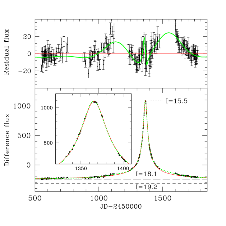
Figure 6.: This is the lightcurve for OGLE 99-BLG-32, a remarkable event in many ways. It is the longest known microlensing event to date. The lower panel shows the difference image flux, together with a standard and a parallax fit. The upper panel shows the residuals (the observed flux minus the standard fit). It demonstrates that a standard fit is unsatisfactory, as it shows systematic discrepancies. However, the parallax fit nicely reproduces the pattern of the deviations [From Mao et al. 2002].

Xallarap Events

Xallarap is a neologism first used in print by Bennett (1998). It is parallax backwards; the xallarap effect is the converse of the parallax. In a xallarap event, there are measurable distortions in the lightcurve caused by the motion of the binary source (e.g., Han & Gould 1997; Dominik 1998). A xallarap event occurs [1] if the Einstein radius projected onto the source plane is of the same size as the binary semimajor axis (${\hat{R}}_{\rm E}\sim a$), and [2] if Einstein crossing time is long compared to the binary period ( $t_{\rm E}\mathrel{\hbox to0.0pt{\lower 3.0pt\hbox{$\sim$}\hss}\raise 2.0pt\hbox{$>$}}\tau$) so that the acceleration of the binary becomes apparent during the course of the event. For such an event, the size of the Einstein ring radius projected onto the source plane ${\hat{R}}_{\rm E}$ is measured by scaling the event against the size of the binary’s orbit (which has to be inferred by other astrophysical means).

An example of a xallarap event is MACHO 96-LMC-2, identified by Alcock et al. (2001a). There are detectable deviations at the maximum of the lightcurve which cause a xallarap fit to be preferred to the standard one. The additional information provided by the xallarap effect suggests that the lens resides in the Large Magellanic Cloud (LMC) rather than the Galactic halo. The binary source has a total mass of $\sim 2$ $M_{\odot}$. In the preferred fit, the primary contributes all the light, while the secondary is a dark companion.

Finite Source Size Effects

When the distance of closest approach is comparable to or smaller than the stellar radius ($u_{0}\mathrel{\hbox to0.0pt{\lower 3.0pt\hbox{$\sim$}\hss}\raise 2.0pt\hbox{$<$}}R_{\star}$), then the source star can no longer be regarded as point-like (Witt & Mao 1994, Gould 1994a). This typically causes measurable distortions to the peak of the event, which may be brighter than or fainter than that for a point source. Another possibility is that the lens may even transit in front of the disk of the source star, which causes inflection points in the lightcurve and hence allows a measurement of the crossing time (Nemiroff & Wickramasinghe 1994).

An example of microlensing event which shows dramatic deviations from the standard Paczyński curve due to finite source size effects is MACHO 95-BLG-30 (Alcock et al. 1997d). This is caused by the transit of the lens across the face of the source star and enables measurement of the lens angular impact parameter in terms of the source size, namely $\theta_{\rm min}/\theta_{\star}$ = 0.7. This information, together with spectroscopic and photometric data, suggests that the source is an M4 star of radius $\sim 60$ solar radii located on the far side of the bulge at $\sim 9$ kpc.

Binary Events

The most common source of deviation is binarity (e.g., Mao & Paczyński 1991). A point lens lightcurve is defined by just three parameters, $t_{0},u_{0}$ and $t_{\rm E}$. A static binary lens is defined by at least six parameters, namely: (i) the projected separation of the binary $d$ in terms of the Einstein radius, (ii) the binary mass ratio $q$, (iii) the Einstein timescale $t_{\rm E}$ associated with the combined mass of the binary, (iv) the angle $\alpha$ at which the source crosses the binary axis, (v) the smallest separation of the source relative to the center of mass $u_{0}$ and (vi) $t_{0}$ which is the time when $u=u_{0}$. Binary microlensing events are important because they are usually accompanied by caustic crossings. A caustic is a curve in the source plane which marks the locus of infinite magnification. If a source passes near or across a caustic, huge changes in magnification can reveal the angular structure of the source (e.g., Gould 1994a; Witt 1995). Modelling of the lightcurve then enables the measurement of $\rho_{\star}=\theta_{\star}/\theta_{\rm E}$. In other words, the angular Einstein ring $\theta_{\rm E}$ is measured by scaling the event against the angular size of the source $\theta_{\star}$, which can be determined from the source flux and colour, together with a colour/surface brightness relation. If the observations are sufficiently detailed, then the intensity variation over the disk of the source star (limb darkening coefficients) may be inferred.

A spectacular example of a binary caustic crossing event is provided by MACHO 98-SMC-1. The source star lies in the Small Magellanic Cloud (SMC). The event was alerted just after the entry into the caustic, and the exit from the caustic was intensively monitored by several groups in five passbands (Afonso et al. 2000). From the lightcurves, the time taken for the caustic to cross the face of the source can be deduced. If the distance of the source can be inferred by astrophysical means, then the projected velocity $v_{\rm p}$ of the lens at the source can be computed. The Galaxy halo’s optical depth peaks at a heliocentric distance of $\sim 10$ kpc and the characteristic lens velocity is $\sim 200\;{\rm kms}^{-1}$, giving a projected velocity at the SMC of $v_{\rm p}\sim 1000\;{\rm kms}^{-1}$. For a lens in the SMC itself, the projection factor is nearly unity, so $v_{\rm p}\sim 50\;{\rm kms}^{-1}$. For comparison, the value of the projected velocity measured from the data on MACHO 98-SMC-1 is $\sim 80\;{\rm kms}^{-1}$. So, the additional information provided by the binary caustic crossing shows that the lens is most likely to be in the SMC than the Galactic halo itself (Kerins & Evans 1999). The wealth of detail also enabled limb darkening coefficients to be computed for five passbands.

Pride of place amongst the exotic events must go to An et al.’s (2002) analysis of EROS 2000-BLG-5, which was the first time that a microlens mass was measured. Here, the degeneracy was completely broken by a combination of exotic effects. The complex light curve of EROS 2000-BLG-5 has three peaks, two being caused by the entrance and exit to a caustic and the third by the source’s close passage to a cusp. This tells us that the lens is a binary. The three photometric peaks allow the source position to be located exactly relative to the lens geometry at three distinct times, thus enabling the Einstein radius projected onto the observer’s plane to be measured using the parallax effect (${\tilde{R}}_{\rm E}\sim 3.6$ AU). Moreover, finite source size effects can be measured during the caustic crossings and fix the ratio of the angular Einstein radius to the angular source size. Given an estimate of the source size from its position on the colour-magnitude diagram, this yields the angular Einstein radius ($\theta_{\rm E}=1.4$ mas). Referring back to eq. (6), we see that the mass of the lens is now completely defined. Accordingly, An et al. (2002) measured the mass as $0.61$ $M_{\odot}$ and concluded that the lens is a low mass disk binary (M dwarf) system about 2 kpc from the Sun. Very recently, Smith et al. (2003) have also carried a mass determination for a microlensing event in the OGLE-II database. This lightcurve too shows both finite source size and parallax effects. The lens mass is $0.05$ $M_{\odot}$, which is interesting as it lies within the brown dwarf régime. However, in this event, the parallax signature is weak, and it is possible that the effect is really caused by a binary source. As Smith et al. (2003) point out, this possibility can be tested by follow-up spectroscopy.

This completes our description of the fundamentals of vanilla and exotic microlensing. In the next three sections, we describe applications of microlensing to studies of dark matter (§3), the structure of the Milky Way and Andromeda galaxies (§4) and limb darkening (§5) in turn.

3. Application I: Dark Matter

3.1. Dark Matter Candidates

The nature of the dark matter haloes surrounding spiral galaxies is a problem of enormous strategic importance in modern physics and astronomy. Baryonic candidates include; (i) black holes, (ii) stellar remnants, such as neutron stars or white dwarfs, (iii) red dwarfs or very faint stars, (iv) brown dwarfs, which are stars made from hydrogen and helium but are too light to ignite nuclear fusion reactions, (v) Jupiters, which are hydrogenous objects with masses $\sim 10^{-3}\,M_{\odot}$, (vi) snowballs, which are compact objects with masses $<10^{-3}\,M_{\odot}$ and held together by molecular rather than gravitational forces and (vii) clouds of molecular hydrogen (e.g, Carr 1994; Evans 2002). Microlensing searches can detect almost all these forms of baryonic dark matter, except diffuse clouds of gas. Non-baryonic candidates include; (i) elementary particles, such as massive neutrinos, axions or neutralinos, (ii) topological defects in a gauge field, and (iii) primordial black holes made out of radiation. Microlensing searches can detect primordial black holes, but not elementary particles or topological defects.

In the early 1990s, a number of authors (Ashman & Carr 1988; Thomas & Fabian 1990) suggested that cooling flows may have occurred at cosmological epochs and that galactic haloes may consist of low mass stars formed in such flows. There even appeared to be supporting evidence from star count data in our Galaxy (Richer & Fahlman 1992). Red and brown dwarfs were therefore foremost candidates for the dark matter in galaxy haloes. In fact, red dwarfs (M and L dwarfs) are the commonest stars in the Galaxy. About $90\%$ of all stars are red dwarfs. They have masses between $\sim 0.5$ $M_{\odot}$ and $\sim 0.08$ $M_{\odot}$, and shine due to hydrogen burning in their cores. Brown dwarfs are objects lighter than $\sim 0.08$ $M_{\odot}$. They are too light to ignite hydrogen. They are brightest when born and then continuously cool and dim. Near-infrared surveys (DENIS and 2MASS) have been discovering abundant brown dwarfs since 1997. Reid et al. (1999) reckoned that the local number density of brown dwarfs is as high as $0.1$ per cubic pc. In which case, the total number of brown dwarfs exceeds the total number of all stars in the Galaxy.

In the early 1990s, by contrast, white dwarfs were regarded as rather improbable dark matter candidates. The main problem is that white dwarfs have masses in the range $\sim 0.5$ $M_{\odot}$, but are remnants of stars with masses in the range 1-8 $M_{\odot}$. So, the manufacture of white dwarfs is necessarily accompanied by the disgorging of substantial amounts of gas and metals into the ISM, whose presence would surely have been detectable by now if the dark matter were comprised of abundant white dwarfs. It also needs a contrived mass function so as to avoid leaving large numbers of visible main sequence precursors still burning today in the halo.

3.2. The MACHO and EROS Experiments

The raw data in a microlensing experiment yield a rate (number of stars microlensed per million stars monitored per year) and a timescale distribution (number of events with timescales between $t_{\rm E}$ and $t_{\rm E}+dt_{\rm E}$). These observables depend on the distribution of masses of the lenses and the distribution of proper motions of the lenses and the sources, all of which are unknown. At first sight, therefore, it seems that little definite can be established from microlensing data. In fact, this is not the case, as a robust quantity can be calculated from the observables. Suppose there is a threshold amplification, say $1.34$, above which microlensing can be detected. This means that the lens lies within an Einstein radius of the line-of-sight between observer and source for a detectable event. Let us imagine a tube of circular cross section whose radius is the Einstein radius (e.g., Griest 1991). So, the tube attains its maximum cross-section half-way between observer and source. The microlensing optical depth $\tau$ is just the number of lenses in this tube

$$\tau={\pi\over M}\int_{0}^{D_{\rm os}}R_{\rm E}^{2}\rho(D_{\rm ol})\,dD_{\rm ol},$$ (11)

where $M$ is the characteristic mass and $\rho$ is the density of lenses. This is independent of the velocities of the lenses and sources by construction. It is also independent of the masses of the lenses (as $R_{\rm E}\propto\sqrt{M}$). The microlensing optical depth is a robust quantity depending only on the lens density distribution, which can be compared against predictions from Galactic models. It has a natural interpretation as the probability that a given star is being microlensed. It can also be calculated directly from the data as a sum over the detected events:

$$\tau={\pi\over 4}\sum_{i}{t_{0,i}\over NT\epsilon(t_{0,i})},$$ (12)

where $N$ is the number of stars monitored, $T$ is the duration of the experiment, $t_{0,i}$ is the timescale of the $i$th event and $\epsilon$ is the efficiency as a function of timescale.

Inspired by Paczyński’s (1986) suggestion, the MACHO and EROS experiments began monitoring millions of stellar images in the Large Magellanic Cloud (LMC) in 1993. From 5.7 years of data, the MACHO collaboration found between 13 to 17 microlensing events and reckoned that $\tau\sim 1.2^{+0.4}_{-0.3}\times 10^{-7}$ (Alcock et al. 2000b). They argued that, interpreted as a dark halo population, the most likely mass of the microlenses is between 0.15 and 0.9 $M_{\odot}$ and the total mass in these objects out to 50 kpc is found to be $9^{+4}_{-3}\times 10^{10}$ $M_{\odot}$. This is $\mathrel{\hbox to0.0pt{\lower 3.0pt\hbox{$\sim$}\hss}\raise 2.0pt\hbox{$<$}}20\%$ of the halo. From 8 years of monitoring the Magellanic Clouds, the EROS collaboration found three microlensing candidates towards the LMC and one towards the SMC (Lasserre et al. 2000). The EROS experiment monitors a wider solid angle of less crowded fields in the LMC than the MACHO experiment, so the two experiments are not directly comparable. Even though EROS do not analyze their data in terms of optical depth, it is clear that their results point to a lower value than that found by MACHO.

Optical depth of the thin disk	$0.15\times 10^{-7}$
Optical depth of the thick disk	$0.04\times 10^{-7}$
Optical depth of the spheroid	$0.03\times 10^{-7}$
Optical depth of the LMC disk (centre)	$0.53\times 10^{-7}$
TOTAL	$0.75\times 10^{-7}$

Table 1.: Inventory of the optical depths of known stellar populations in the outer Galaxy or the Large Magellanic Cloud (taken from Alcock et al. 1997b).

The first question to ask is: have the MACHO and EROS experiments detected any signal of the dark halo whatsoever? There are a number of known stellar populations in the outer Galaxy and the LMC that contribute to the microlensing optical depth, as listed in Table 1. Of these, only the optical depth of the LMC remains controversial, with a number of authors arguing for significantly higher values (e.g., Sahu 1994; Evans & Kerins 2000). Even using the conservative value given in Table 1, the microlensing optical depth caused by known stellar populations is $\sim 0.75\times 10^{-7}$, which is within $2\sigma$ of the value deduced from the 5.7 yr MACHO observations. There may even be hitherto undetected populations in the outer Galaxy or the LMC – such as tidal debris (Zhao 1998), the warped outer Milky Way disk (Evans et al. 1998) or an intervening dwarf galaxy (Zhao & Evans 2001). Hence, it is possible that the microlensing signal comes entirely from foreground or background populations and has nothing to do with the dark halo at all. This viewpoint is supported by the evidence from the exotic events. There are now four such events (two binary caustic crossing events, one long timescale event with no detectable parallax, one xallarap event) for which the location of the event can be more-or-less inferred. In all cases, the lens most likely resides in the Magellanic Clouds. Most recently of all, there has been the direct imaging of a lens by Alcock et al. (2001b), revealing it to be a nearby low-mass star in the disk of the Milky Way.

The second question to ask is: if we do assume that the lenses lie in the dark halo, what are they? Red dwarfs are ruled out because they are not seen in sufficient numbers in long exposures of high latitude wide-field camera Hubble Space Telescope fields. Specifically, less than $1\%$ of the mass of the halo can be in the form of red dwarfs (Bahcall et al. 1994; Graff & Freese 1996). Brown dwarfs are ruled out because the timescales of the microlensing events are too long. By examining different velocity anisotropies and rotation, Gyuk, Evans & Gates (1998) showed that the minimum mass of the microlensing objects must be $\mathrel{\hbox to0.0pt{\lower 3.0pt\hbox{$\sim$}\hss}\raise 2.0pt\hbox{$>$}}0.1$ $M_{\odot}$, which lies above the hydrogen-burning limit. So, despite their abundance in the Galaxy, both brown and red dwarfs cannot be the culprits. White dwarfs remain possible, at least as regards the timescales. The MACHO collaboration favoured an explanation in which $\mathrel{\hbox to0.0pt{\lower 3.0pt\hbox{$\sim$}\hss}\raise 2.0pt\hbox{$<$}}20\%$ of the dark halo was built of white dwarfs. However, this has been fiercely contested by others as being inconsistent with other pieces of astrophysical evidence. For example, the existence of multi TeV $\gamma$-rays from Makarian 501 places a powerful constraint on white dwarfs, as their progenitors would produce infrared radiation that can interact to produce electron-positron pairs (Graff et al. 1999). More directly, overproduction of carbon, nitrogen, deuterium and helium are all in serious conflict with observations unless the contribution to the critical density from white dwarfs $\Omega_{\rm WD}$ is less than $0.003$ (Fields, Freese & Graff 2000).

3.3. Conclusions

Despite such controversies, microlensing has told us a crucial fact about the Galactic dark halo. Almost all the dark halo is not built from stellar or sub-stellar compact objects. A whole swathe of baryonic dark matter candidates are ruled out as dominant contributors. The constraints from the spike (or short timescale) analysis on Jupiters and snowballs are particularly severe. The only baryonic dark matter contenders that remain possible are supermassive black holes and clouds of diffuse gas. Of course, particle dark matter does not cause microlensing events and remains the most likely solution of all.

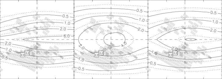
Figure 7.: Contours of microlensing optical depth to the red clump giants (in units of $10^{-6}$) in three barred Galaxy models, excluding (full lines) and including (dotted lines) spirality. The optical depths reported by Alcock et al. (2000a) and Popowski et al. (2000) are shown in boxes. Light (dark) gray boxes correspond to EROS (OGLE II) fields [From Evans & Belokurov 2002].

4. Application II: Galactic Structure

4.1. The Milky Way

Microlensing surveys towards the Bulge were originally proposed by Paczyński (1991) and Griest et al. (1991) as a check on the reliability of the searches towards the LMC. They have now evolved into uniquely important probes of the mass distribution in the inner Galaxy. Conventional models of the barred inner Galaxy are derived from the stellar kinematics, motions of atomic and molecular gas, starcount data and measurements of integrated light (e.g., Binney et al. 1991; Häfner et al. 2000). Such datasets therefore measure either the light distribution or the gravity field and so they lack the immediacy of microlensing surveys, which alone measure the mass distribution directly.

In fact, the early calculations by Paczyński and Griest assumed that the main lensing population was foreground disk stars. They concluded that the optical depth to the Galactic Center was of the same order as that towards the LMC ($\tau\sim 4\times 10^{-7}$). The first OGLE and MACHO observational results, although based on small samples, showed that this was clearly in error (Udalski et al. 1994; Alcock et al. 1995) and that the optical depth was about an order of magnitude higher ($\tau\sim 3\times 10^{-6}$). The important breakthrough was made by Kiraga & Paczyński (1994), who first deduced that the main lensing population was not the disk stars, but the bulge stars themselves. Early on, too, it was realised that such high values of the optical depth doomed purely axisymmetric models of the inner Galaxy and strongly favoured barred models (Paczyński et al. 1994; Evans 1994, 1995). Nonetheless, a neat match between the data and the models continued to elude investigators, until finally Binney, Bissantz & Gerhard (2000) raised the alarum with a paper entitled: “Is Microlensing Compatible with Galactic Structure?”. They argued that the values of the optical depth for microlensing to bulge sources – in particular, the Alcock et al. (2000a) value of $\tau=3.23\times 10^{-6}$ – were so high that they were in conflict with barred models derived from infrared surveys and gas motions. Fig. 7 shows contours of optical depth to bulge sources computed for three popular models of the inner Galaxy (Evans & Belokurov 2002). All three models (Binney, Gerhard & Spergel 1997; Freudenreich 1998; Dwek et al. 1995) are derived from the infrared emissivity measured by the DIRBE instrument on the COBE satellite, but make different corrections for the distribution of dust. As can been seen, bar models such as Binney et al.’s and Dwek et al.’s cannot reproduce the high value of $\tau=3.23\times 10^{-6}$ at Galactic longitude and latitude ($\ell=2.68^{\circ},b=-3.35^{\circ}$). Both these models are highly concentrated towards the Galactic plane. By contrast, Freudenreich’s model is more massive and swollen, and so gives values of the optical depth close to the observations. However, in constructing his model, Freudenreich (1998) masked out most regions close to the Galactic plane ($|b|<5^{\circ}$) as being anomalously reddened by dust. So, the model is perhaps untrustworthy near the plane, as it depends heavily on uncertain extrapolations from the outer parts.

Collaboration	Location	Optical Depth	Method
Udalski et al. (1994)	Baade’s Window	$\sim 3.3\times 10^{-6}$	PSF ($f_{d}=0.0$)
Alcock et al. (1995)	($2.3^{\circ},-2.65^{\circ}$)	$\sim 3.9\times 10^{-6}$	PSF ($f_{d}=0.0$)
Alcock et al. (1997a)	($2.5^{\circ},-3.64^{\circ}$)	$3.9^{+1.8}_{-1.2}\times 10^{-6}$	Red Clump
Alcock et al. (2000a)	($2.68^{\circ},-3.35^{\circ}$)	$3.23^{+0.52}_{-0.50}\times 10^{-6}$	DIA ($f_{d}=0.25$)
Popowski et al. (2002)	($3.9^{\circ},-3.8^{\circ}$)	$2.0\pm 0.4\times 10^{-6}$	Red Clump
Popowski (2003)	($2.2^{\circ},-3.2^{\circ}$)	$2.2^{+0.4}_{-0.4}\times 10^{-6}$	DIA ($f_{d}=0.1$)
Sumi et al. (2003)	($3.0^{\circ},-3.8^{\circ}$)	$3.40^{+0.94}_{-0.73}\times 10^{-6}$	DIA ($f_{d}=0.25$)
Afonso et al. (2003)	($2.5^{\circ},-4.0^{\circ}$)	$0.94\pm 0.26\times 10^{-6}$	Red Clump

Table 2.: The microlensing optical depth recorded by various experimental groups towards locations in the Galactic bulge. The method used by each collaboration is also given (DIA = difference image analysis, PSF = conventional point spread function photometry, such as SoDoPHOT). If the red clump method is not used, then the fraction of disk sources $f_{d}$ must be estimated.

Table 2 lists the values of the optical depth to sources in the bulge as measured by a number of investigators. The best way to measure this is to use the sub-sample of microlensing events of the red clump sources only. This is because the red clump stars are known to reside in the bulge and because they are so bright that the efficiency depends only on the temporal sampling. Another way is to measure the optical depth to all sources – whether by using difference image analysis (DIA) or conventional point spread function (PSF) photometry – and then to correct the total optical depth by the fraction of disk sources $f_{d}$. This requires the efficiency of the entire experiment to be computed, as well as $f_{d}$ to be estimated from theoretical models. Table 2 shows that the optical depth computed from the red clump stars is lower than than that computed by correcting the total optical depth (aside from the early values which depend on a handful of events). The origin of this trend remains unexplained.

The recent, very high result of $\tau\sim 3.4\times 10^{-6}$ from the MOA collaboration (Sumi et al. 2003) maintains the inconsistency between microlensing and galactic structure. This value is in fact still higher than that reported by Alcock et al. (2000a) and is measured at a location still further from the Galactic Center. All three models in Fig. 7 fail to achieve this number by a good margin. However, there is also a recent, very low result of $\tau\sim 0.94\times 10^{-6}$ from the EROS collaboration (Afonso et al. 2003) using the red clump method. In fact, this number can be reproduced rather easily even by Binney et al.’s model (the least massive and swollen of the bars in Fig. 7). These two most recent determinations – amongst the highest and lowest ever reported – suggest that the systematics in these experiments are still not properly understood.

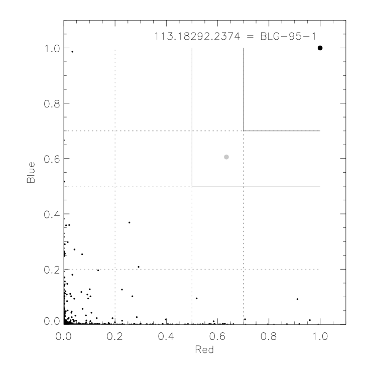
Figure 8.: The results of processing a tile of MACHO data towards the Galactic Bulge. The posterior probability of microlensing given the blue data is plotted against the same probability given the red data. There is a single microlensing candidate identified by MACHO on the tile, namely BLG-95-1. It is also cleanly identified by the neural network as the black spot in the top right hand corner. Note that the neural network filters almost all the variable stars, which are in the bottom left hand corner. There is however one pattern marked by a grey spot which lies in the regime of novelty detection. Close inspection of the network shows that it is probably a noisy lightcurve of an eruptive variable [From Belokurov, Evans & Le Du 2003].

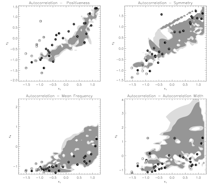
Figure 9.: The locations of 36 microlensing events (from Alcock et al. 2000a) in the input space ($x_{1},x_{2},x_{3},x_{4},x_{5}$). These parameters describe the five characteristic features of microlensing events, namely (i) an excursion from the baseline that is (ii) positive, (iii) symmetric, (iv) single and controlled by (v) a timescale. Also shown are the contours of posterior probability of microlensing for the training sets in the input space. Light gray means that the probability is greater than 0.5. Dark gray means that the probability is greater than 0.9 and corresponds to almost certain microlensing. The 36 microlensing events were originally identified by Alcock et al. (2000a) on the basis of conventional PSF photometry. The microlensing nature of the events represented by circles coloured black is corroborated by the network, but those represented by circles coloured white is not. There are 11 events not identified as microlensing when the red data is fed into the neural network [From Belokurov, Evans & Le Du 2003].

One possibility is that the selection of events is too lax and that background supernovae and forms of stellar variability are being inadvertently identified as microlensing. Although the microlensing phenomenon has a number of characteristic signatures (e.g., achromaticity, symmetry, uniqueness), these can be undermined in heavily crowded fields where blending occurs, or in the case of sparse and noisy sampling. A recent development has been the exploitation of neural networks to discriminate between the shapes of microlensing lightcurves and other contaminants, such as variable stars. Belokurov, Evans & Le Du (2003) present a working neural network to identify microlensing. It has five input neurons, a hidden layer of five neurons and one output neuron. Microlensing events are characterised by the presence of (i) an excursion from the baseline that is (ii) positive, (iii) symmetric, (iv) single and (v) a timescale. Motivated by this, five parameters are extracted by spectral analysis from the lightcurves and fed to the neural networks as inputs. The output of the network is the posterior probability of microlensing. For example, Fig. 8 shows the results of processing all lightcurves in MACHO tile 18292 of field number 113, which lies towards the Galactic bulge. This tile contains $\sim 5000$ lightcurves, of which one was identified by MACHO as a microlensing event. The data are taken at a site with median seeing of $\approx 2.1^{\prime\prime}$. This means that the quality of the data is sometimes poor. Each lightcurve is presented to the neural network, with the red and blue passband data analysed separately. It would be preferable to analyze the red and blue data together because most variable stars show colour differences. However, this option is not viable at the moment because the publically available colour information on variable stars is still quite limited. Fig. 8 shows the results of the deliberations of the neural network. The probability of microlensing given the blue data is plotted against the probability given the red data. There is only one pattern that is unambiguously identified, namely the event designated by MACHO as BLG-95-1. It is clearly and cleanly separated from the rest of the patterns as a black circle in the topmost right corner. There is an additional pattern that has output values $y\approx 0.6$ for both the red and blue data. This falls within the regime of novelty detection. It is most probably a form of stellar variability that the network has not previously met in its training phase.

Such tests give confidence that the neural network approach is a fruitful one. When applied to a larger sets, however, there are some discrepancies between events identified by MACHO and those identified by neural networks. For example, Alcock et al. (2000a) identified 36 events towards the Galactic Bulge on the basis of a series of photometry and colour cuts applied to the lightcurves. The neural network finds a total of 19 events identified with a probability $\mathrel{\hbox to0.0pt{\lower 3.0pt\hbox{$\sim$}\hss}\raise 2.0pt\hbox{$>$}}0.9$ as microlensing in both the red and blue filters. Additionally, there are 2 events securely identified in the blue data, but not in the red; there are 6 events identified in the red data, but not in the blue. Lastly, there are 9 events for which no microlensing signal whatsoever is detected. This suggests that the MACHO group’s classification algorithm is itself probably not 100 per cent efficient. Fig. 9 shows the contours of probability for the training set in the input space. Light gray means that the probability is greater than 0.5 and corresponds to the formal decision boundary. Dark gray means that the probability is greater than 0.9 and corresponds to almost certain microlensing. The events identified in the red passband are designated by filled circles, events missed are open circles.

In fact, the identification of microlensing events is much more difficult than usually acknowledged. It probably lies at the heart of the seeming discord between microlensing and Galactic structure in the inner Galaxy, as well as the seeming discord between the MACHO and EROS experiments towards the Large Magellanic Cloud. In order that microlensing surveys achieve their true status as the most powerful probe of galactic structure, the identification problem will need to be much more thoroughly understood than at present.

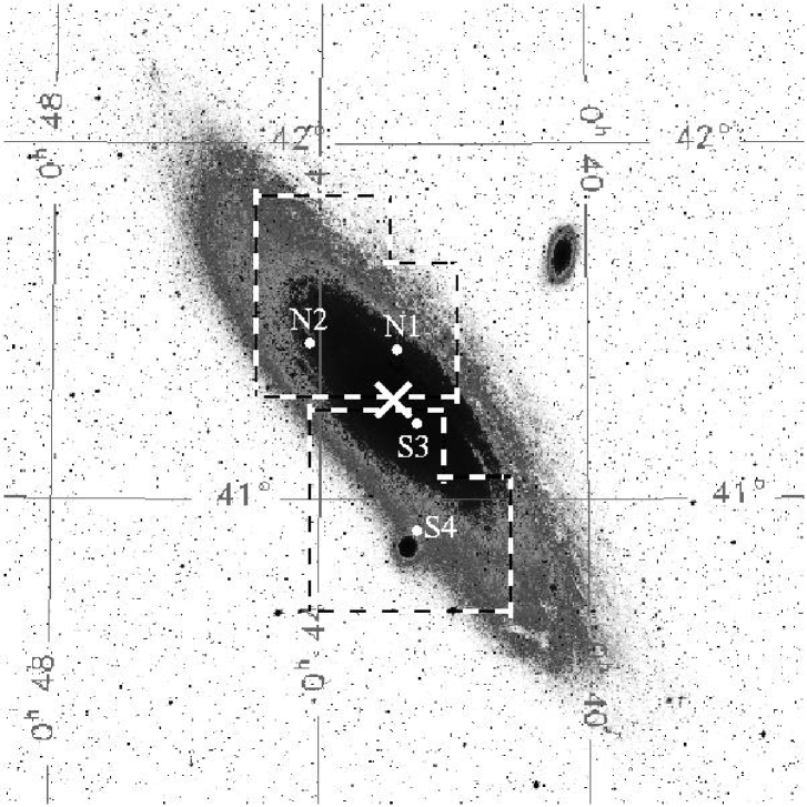
Figure 10.: The location of the 4 microlensing candidates detected by POINT-AGAPE towards M31. Also marked are the two INT fields that straddle the north and south of M31 [From Paulin-Henriksson et al. 2003].

reference	$\Delta R$ (mags)	$t_{1/2}$ (days)	$t_{E}$ (days)	$A_{\rm max}$
PA-99-N1	$20.8\pm 0.1$	1.9	$9.74\pm 0.70$	$17.54^{+1.33}_{-1.15}$
PA-99-N2	$19.0\pm 0.2$	25.0	$91.91^{+4.18}_{-3.83}$	$13.33^{+0.75}_{-0.67}$
PA-00-S3	$18.8\pm 0.2$	2.3	$12.56^{+4.53}_{-3.23}$	$18.88^{+8.15}_{-5.89}$
PA-00-S4	$20.7\pm 0.2$	2.1	$128.58^{+142.61}_{-72.27}$	$211^{+16456}_{-120}$

Table 3.: Parameters for the 4 POINT-AGAPE candidates. Here, $\Delta R$ is the magnitude (Johnson/Cousins) of the maximum source flux variation, $t_{E}$ is the Einstein timescale, $t_{1/2}$ is the full-width half-maximum and $A_{\rm max}$ is the maximum amplification. All these events have very high amplification and short full-width half-maximum timescale [From Paulin-Henriksson et al. 2003].

4.2. The Andromeda Galaxy

The Andromeda Galaxy (M31) is now the subject of intense scrutiny by a number of groups (e.g., Aurière et al. 2001; Riffeser et al. 2001; Calchi-Novati et al. 2001; Crotts et al. 2001; Paulin-Henriksson et al. 2002, 2003). Conventional microlensing is limited to the only three galaxies in which there are large numbers of resolved stars (the Milky Way, the LMC and the SMC). In M31, the potentially lensed stars are much fainter than the integrated light from all the stars within the seeing disk. So, the observed quantity is the lightcurve associated with the flux on a pixel or super-pixel. This technique is known as pixel lensing (e.g., Gould 1996a). It is no longer possible to measure the unlensed fluxes of the individual sources, nor the timescales of individual events. Rather, an event is characterised by its full-width half-maximum timescale $t_{1/2}$ which is only crudely related to the mass of the lens. Pixel lensing represents the ultimate limit of scientific detection because not only is the lens invisible, but so in essence is the source (because it cannot be distinguished from other stars in the same pixel). The success of the technique rests upon the variation in the brightness of the source manifesting itself as a variation in the local surface brightness. This is potentially a very powerful technique, which offers “the key to the Universe” (Gould 1996b) or at least the key to the nearest 50 Mpc (Binney 2000).

The POINT-AGAPE collaboration (e.g., Aurière et al. 2001; Kerins et al. 2001) has been conducting a major program of observations using the Isaac Newton Telescope Wide-Field Camera from 1999 to 2002. They monitored nightly two fields in two colours near the central bulge of M31, as shown in Fig. 10. The two fields are each $34^{\prime}\times 34^{\prime}$ and provide a grand total of 256 million pixel lightcurves. The original impetus for the POINT-AGAPE experiment was to detect an asymmetry in the gradients of microlensing events between the near or northern side and the south or furthest side (Crotts 1992, Baillon et al. 1993). This effect arises because the disk of M31 is highly inclined ($i=77^{\circ}$). An asymmetry is produced if most of the microlensing events are caused by compact objects in a spherical halo, as lines of sight to the further, southern side are longer than lines of sight to the nearer, northern side. This asymmetry is not caused by stellar lenses in M31 or foreground lenses in the Milky Way.

As the POINT-AGAPE data are taken on different nights with different photometric conditions, the challenge in the experiment is to eliminate all sources of variation extrinsic to the source. The pixel method (Ansari et al. 1997, 1999; Paulin-Henriksson 2002) has been developed to cope with the measurement of flux changes of unresolved stars in the face of seeing variations. After geometric alignment, the current frame is photometrically corrected to the reference image

$${\overline{\phi}}_{\rm ref}=a{\overline{\phi}}_{\rm cur}+b.$$ (13)

Here, $a$ is the ratio of absorptions (due to variations in airmass or atmospheric transmissions) and $b$ the difference in sky backgrounds. The ${\overline{\phi}}$ values refer to the median flux on a pixel computed using a running window of size $41\times 41$ pixel. The parameters $a$ and $b$ are calculated using the means and dispersion of the current frame as compared to the reference image

$$\sigma^{2}_{\rm ref}=a^{2}\sigma^{2}_{\rm cur},\qquad\qquad\langle\phi_{\rm ref}\rangle=a\langle\phi_{\rm cur}\rangle+b.$$ (14)

Here, the means and dispersions are taken over windows of $500\times 500$ pixels, so as to render any photon noise negligible.

In the pixel method, which is a simple but effective form of difference imaging, each elementary pixel is replaced by a super-pixel centered upon it. Each super-pixel is a square of 7 $\times$ 7 pixels. The size of the super-pixel must be chosen empirically so as to be large enough to cover the whole seeing disk, but not so large that any variation is diluted. If each pixel were weighted with the point spread function, whose width was allowed to vary with the seeing, then this method would be equivalent to a difference image analysis, as utilised by Tomaney & Crotts (1996). The simpler super-pixel method corrects for the different loss of flux in the changing wings of the PSF with the changing seeing by using an empirical “seeing stabilisation” (e.g, Paulin-Henriksson 2002). This is deduced by looking at the correlation between the differences in the super-pixel flux and its median on the current and reference image, namely

$$\phi_{\rm cur}-{\overline{\phi}}_{\rm cur}=(1+\alpha)\left(\phi_{\rm ref}-{\overline{\phi}}_{\rm ref}\right)+\beta.$$ (15)

Here, ($\alpha,\beta$) are estimated by using all the super-pixels on the current frame. They are then used to correct the current super-pixel flux to the reference seeing, viz

$$\phi={a\left(\phi_{\rm cur}-{\overline{\phi}}_{\rm cur}\right)-\beta\over\alpha+1}+{\overline{\phi}}_{\rm ref}.$$ (16)

This gives the photometrically and geometrically aligned, stable flux. Although crude, this procedure strikes a nice balance between computational efficiency and optimal signal-to-noise, with the resulting noise level approaching the photon noise limit.

The POINT-AGAPE collaboration has thus far processed the first two years of data and has a list of 362 candidate microlensing events (Paulin-Henriksson et al. 2003). These pass the sequence of cuts required to isolate candidate events. However, many of these are probably variable stars and will require additional baseline data before they can be distinguished from microlensing. For the moment, POINT-AGAPE have restricted themselves to high amplitude events with full-width half-maximum timescales $t_{1/2}$ shorter than 25 days. These cuts eliminate almost all of the troublesome long-period Mira variables that are the most serious contaminants in this experiment. This leaves four, robust high signal-to-noise events (PA-99-N1, PA-99-N2, PA-00-S3, PA-00-S4), whose characteristics are listed in Table 3 and whose locations are marked on Fig. 10. Here, 99 and 00 designate the year in which the event reached maximum, while N and S indicate whether the event occurred in the northern or the southern field.

Remarkably, all the events that have thus far been discovered can reasonably enough be ascribed to stellar lenses. The projected positions of PA-99-N1 and PA-00-S3 lie within the bulge of M31, where lensing by stars in M31 overwhelmingly dominates over lensing by objects in the halo. The projected position of PA-00-S4 lies very close to the centre of the foreground elliptical galaxy M32. The detailed analysis of this event by Paulin-Henrikkson et al. (2002) suggests that the source star lies in the M31 disk, but that the lens most probably resides in M32 itself. For example, the optical depth to lensing by M32 stars is $\tau\sim 1.4\times 10^{-6}$, which is roughly twice as big as the optical depth to compact, dark objects in M31’s halo (assuming Alcock et al.’s (2000b) value of 20 % as the fraction in such objects). The event PA-99-N2 lies in the disk $\sim 22^{\prime}$ from the centre of M31. However, its Einstein crossing time is $\sim 92$ days, making it the longest event so far discovered in the direction of Andromeda. A microlensing event with a short Einstein crossing time far out in the disk would be an unambiguous candidate for a dark halo lens. Given the long timescale, the most likely interpretation is that the lens is also a disk star, and that this is an example of disk-disk lensing (e.g., Gould 1994b). The optical depth to disk-disk lensing at this location is $\sim 10^{-7}$, which is of the same order as the M31 halo under the Alcock et al. 20 % hypothesis.

What is intriguing is that none of the existing candidates seemingly implicates a lens in M31’s halo. Rather, they seem to suggest that the main lensing populations coincide with the known stellar populations. If this trend persists, then the experiments towards M31 have the potential to test whether mass traces light in the M31 bulge and disk. Such hypotheses are frequently used in galactic modelling, but have so far never been checked.

5. Application III: Limb Darkening

Limb darkening is the name given to the darkening at the rim of the stellar disk. It is familiar from optical images of the Sun, in which context it has been extensively studied. It happens because photons on lines of sight towards the rim emanate from less deep, and hence cooler, layers of the Sun than photons on lines of sight towards the centre. Measurements of limb darkening in stars other than the Sun would provide a useful check on theories of stellar atmospheres. However, such measurements are hard to carry out with conventional techniques.

In a binary lens, a caustic is an extended structure. If the source passes near or across the caustic, drastic changes in the magnification can reveal the finite size and the surface brightness profile of the source. This opens up the possibility of studying limb darkening with gravitational microlensing, as envisaged originally by Bogdanov & Cherepaschuk (1995), Witt (1995) and Valls-Gabaud (1998). This technique has been spectacularly exploited in recent years by the PLANET collaboration.

The phenomenon of limb darkening is normally parametrised according to either a linear law

$$S_{\lambda}(\vartheta)={\overline{S}_{\lambda}}\left[(1-\Gamma_{\lambda})+{3\Gamma_{\lambda}\over 2}\cos\vartheta\right],$$ (17)

or a square-root law

$$S_{\lambda}(\vartheta)={\overline{S}_{\lambda}}\left[(1-\Gamma_{\lambda}-\Lambda_{\lambda})+{3\Gamma_{\lambda}\over 2}\cos\vartheta+{5\Lambda_{\lambda}\over 4}\cos^{1/2}\vartheta\right].$$ (18)

In these formulae, $S_{\lambda}$ is the surface brightness of the star as a function of $\vartheta$, which is the angle between the normal to the stellar surface and the line of sight. Additionally, $\Gamma_{\lambda}$ and $\Lambda_{\lambda}$ are the limb darkening coefficients, while ${\overline{S}_{\lambda}}$ is the mean surface brightness. This is related to the total flux received $F_{\lambda}$ via ${\overline{S}_{\lambda}}=F_{\lambda}/(\pi\theta_{\star}^{2})$ where $\theta_{\star}$ is the angular radius of the star. Depending on the quality of the data, it may be feasible to extract either one ($\Gamma_{\lambda}$) or two ($\Gamma_{\lambda}$ and $\Lambda_{\lambda}$) limb darkening coefficients. Of course, the coefficients are a function of the waveband of observation.

A source inside a caustic will be imaged into 5 images; outside the caustic it will be imaged into 3 images. At the caustic, 2 images appear or disappear. These images are infinitely magnified. In the immediate neighbourhood of a caustic, the magnification of the two new images diverges as (e.g., Schneider & Weiss 1986)

$$A\propto\left({1\over\Delta u_{\perp}}\right)^{1\over 2}H(\Delta u_{\perp}),$$ (19)

where $\Delta u_{\perp}$ is the perpendicular separation of the source from the caustic in units of the angular Einstein radius $\theta_{\rm E}$, and $H$ denotes the Heaviside step function. Thus, the magnification of an extended, limb darkened source is just

$$A_{\lambda}={1\over F_{\lambda}}\int\int_{\cal D}d^{2}\vartheta A(\vartheta)S_{\lambda}(\vartheta),$$ (20)

where $F_{\lambda}$ is the total flux. By substituting in the limb darkening laws [eqs. (17) or (18)], the angular integration can be performed analytically to yield (e.g., Appendix B of Albrow et al. 1999b)

$$A=\left({1\over\rho_{\star}^{1/2}}\right)\left[G_{0}(-\Delta u_{\perp}/\rho_{\star})+\Gamma_{\lambda}F_{1/2}(-\Delta u_{\perp}/\rho_{\star})+\Lambda_{\lambda}F_{1/4}(-\Delta u_{\perp}/\rho_{\star})\right],$$ (21)

where $\rho_{\star}=\theta_{\star}/\theta_{\rm E}$ and $G_{0},F_{1/2}$ and $F_{1/4}$ are known functions, specifically

$$G_{n}(\eta) = {1\over B(n+3/2,1/2)}\int_{\rm max(\eta,-1)}^{1}{dx(1-x^{2})^{n+1/2}\over(x-\eta)^{1/2}}H(1-\eta),$$

$$F_{n}(\eta) = G_{n}(\eta)-G_{0}(\eta).$$ (22)

Here, $B(x,y)=\Gamma(x)\Gamma(y)/\Gamma(x+y)$ is Euler’s Beta function. Therefore, by decomposing into basis functions the magnification changes of the source as it crosses the caustic , the limb darkening coefficients $\Gamma_{\lambda}$ and $\Lambda_{\lambda}$ can be extracted.

There are six parameters of a static binary lens. In addition, there are also the source flux, the background flux and the limb darkening coefficients for each waveband. This leads to a $\chi^{2}$ minimization in at least a nine-dimensional parameter space. In practice, it is easier to proceed by transforming from position-magnification space to time-flux space assuming rectilinear motion of the source relative to the lens. This leads to an analytic approximation to the shape of the caustic crossing. The caustic crossing fit then constrains the search for a full solution to a four-dimensional submanifold of the whole nine-dimensional space (Albrow et al. 1999b).

Microlensing is the only technique available to us for studying the limb darkening of distant stars. The recent years have seen limb darkening coefficients measured for two K giants in the bulge (Albrow et al. 1999a, Albrow et al. 2000), for a late G or early K sub-giant in the bulge (Albrow et al. 2001) and for an A dwarf in the SMC (Afonso et al. 2000). Theories of stellar atmospheres predict limb darkening laws for different types of stars. Typically the results seem to show good agreement with theoretical predictions in the V band, but poorer agreement in the I band – as, for example, in OGLE 99-BLG-23 studied by Albrow et al. (2001).

6. The Future

In this concluding final section, we suggest four projects for the next decade.

6.1. K band Microlensing Towards the Bulge

Microlensing surveys in the K band towards the Bulge would be extremely valuable (Gould 1995; Evans & Belokurov 2002). This is all the more true given the capabilities of the new generation of survey telescopes. For example, VISTA  has a field of view of 0.25 square degrees in the K band. Assuming that the seeing is $0.8^{\prime\prime}$ in Chile and scaling the results of Gould (1995), then we estimate that VISTA will monitor $\sim 1.5\times 10^{6}$ stars in a single field of view for crowding-limited K band images towards the Bulge. This means that we are probing the luminosity function down to $K\sim 16$, assuming 3 magnitudes of extinction. We estimate that photometry accurate to $3\%$ for a $K\sim 16$ star will take about 1 minute on VISTA. Hence, a K band survey of a $5^{\circ}\times 5^{\circ}$ field close to the Galactic Center will take about 1.5 hours of time every night. This makes a K band microlensing survey of the inner Galaxy an attractive and feasible proposition with VISTA.

The scientific returns of a K band microlensing survey towards the Bulge will be substantial. First, it will provide new and reliable estimates of the microlensing optical depth for many locations throughout the Bulge, rather than the isolated windows available in the optical bands. Second, the shapes of the contours of optical depth – the microlensing maps – will enable us to discriminate between bar models, such as those highly concentrated towards the Galactic plane (like Binney et al.’s) or those that are diffuse and swollen (like Freudenreich’s).

6.2. Pixel Lensing Towards M33

M33 is a low luminosity spiral galaxy in the Local Group. From the point of view of dark matter studies, it is an interesting target, as it is known that the dark matter content of low luminosity and dwarf galaxies is different from that of big bright galaxies (e.g., Evans 2000). From the behaviour of the rotation curve near the centre, it is clear that dark matter must dominate even the central parts of M33 (Toomre 1981). This is very different from both the Milky Way and M31, which are dominated by luminous matter within the inner few kpc.

The VLT Survey Telescope (VST) has a pixel size of 0.24 arcsec/pixel and a field of view of 1 square degree. VST is likely to see first light in 2003. The likely pixel lensing rate can be crudely estimated as (see e.g., equation (19) of Ansari et al. 1997)

$$N_{\rm ev}\sim 160\times 10^{-0.2(\mu_{\rm gal}-\mu_{\rm M31})}\biggl{(}{\Omega_{\rm gal}\over 1{\rm deg}^{2}}\biggr{)}\biggl{(}{{\rm season}\over 6\ {\rm months}}\biggr{)}\biggl{(}{{\rm seeing}\over 1.5^{\prime\prime}}\biggr{)}^{-1/2},$$

where the normalisation has been determined by Kerins et al.’s (2000) simulations for the campaign on the INT WFC towards M31. Here, $\Omega_{\rm gal}$ and $\mu_{\rm gal}$ are the target galaxy’s solid angle and mean surface brightness respectively. For M33, $\mu_{\rm gal}$ is 23.8 mag arcsec^-2 and $\Omega_{\rm gal}$ is 0.6 ${\rm deg}^{2}$. Paranal in Chile, where the VST is based, has an average seeing of $0.6^{\prime\prime}$. We take 21.5 mag arcsec^-2 as the average surface brightness of M31 within the INT fields. Using our formula, this means that for M33, there will be about 50 events per season for a halo full of substellar compact objects. Taking Alcock et al.’s (2000b) baryon fraction of $20\%$ as applicable, then there will be $\sim 10$ events per season.

Low luminosity spiral galaxies have very different properties to bright spiral galaxies like the Milky Way. The MACHO and EROS experiments have demonstrated that the substellar compact objects are not the dominant contributor to the Milky Way’s dark halo. However, this conclusion cannot be extended to low luminosity galaxies like M33 without further experiments. Hence, a pixel lensing survey of M33 is a very worthwhile project in the context of dark matter science.

6.3. Polarimetry of Microlensing Alerts

A number of theoretical studies have examined polarization changes during microlensing (Simmons, Willis & Newsam 1995; Agol 1996; Belokurov & Sazhin 1997), but no attempts have been made to detect this phenomenon observationally yet. In microlensing, the total flux is partially polarized and the plane of polarization is perpendicular to the plane joining the centres of the source and the lens. As the lens and source are in relative motion, the plane of polarization rotates during the course of the event. For a point lens, the polarization has a magnitude of at most $0.1\%$. However, polarizations as high as $1\%$ can be achieved if the star crosses a caustic in a binary lens. By comparison, the first detection of limb polarization in Algol was at a magnitude of $0.004\%$ (Kemp et al. 1983). Hence, the effect is well within the grasp of current instruments.

The measurement of variable polarization yields the Einstein radius of the lens (if the radius of the star is known or can be estimated) and the velocity direction of the lens projected onto the sky. For a binary lens event, studies of the polarization give the position angle of the binary as well. Stars with high surface temperature are the most promising candidates for observing polarization as electron scattering dominates the opacity (Chandrasekhar 1960; Agol 1996). Measurements of polarization can provide confirmation of the microlensing nature of an event, and enable theoretical calculations of polarization in model stellar atmospheres to be checked and calibrated. Most importantly, the additional information provided by polarimetry for some exotic events may lead to determinations of the mass of the lens. It would therefore be worthwhile to follow up a subsample of, say, $\sim 50$ microlensing alerts with polarimetry.

6.4. Astrometric Microlensing with GAIA

GAIA  is the European Space Agency satellite now selected as a Cornerstone 6 mission. It is the successor to the pioneering Hipparcos satellite, which flew from 1989 to 1993. GAIA is a survey satellite that provides multi-colour, multi-epoch photometry, astrometry and spectroscopy on all objects brighter than $V\approx 20$ (e.g., ESA 2000; Perryman et al. 2001). The dataset is gigantic, as there are over a billion objects in our Galaxy alone brighter than 20th magnitude. A small fraction of the objects monitored by GAIA will show evidence of microlensing. GAIA can observe photometric microlensing by measuring the amplification of a source. However, GAIA is inefficient at discovering photometric microlensing events, as the sampling of individual objects is relatively sparse (there are a cluster of observations once every two months on average).

GAIA is better at detecting astrometric microlensing. The all-sky source-averaged astrometric microlensing optical depth is $\sim 10^{-5}$, which is over an order of magnitude greater than the photometric microlensing optical depth. There are two main difficulties facing GAIA in exploiting this comparatively high probability. First, the astrometric accuracy of a single measurement by GAIA depends on the source magnitude and degrades at magnitudes fainter than $V\approx 15$. Second, GAIA provides a time-series of one-dimensional astrometry by scanning great circles on the sky. The observed quantity is the CCD transit time for the coordinate along the scan. This is the same way the Hipparcos satellite worked (ESA 1997). From the sequence of these one-dimensional measurements, the astrometric path of the source, together with any additional deflection caused by microlensing, must be recovered.

Simulations by Belokurov & Evans (2002) suggest that $\sim 25000$ sources will exhibit astrometric microlensing events during the course of the 5 year mission. The cross-section for astrometric microlensing favours nearby lenses. The most valuable events are those for which the Einstein crossing time $t_{\rm E}$, the angular Einstein radius $\theta_{\rm E}$ and the relative parallax of the source with respect to the lens $\pi_{\rm sl}$ can all be inferred from GAIA’s datastream. The mass of the lens then follows directly. If the source distance is known – for example, if GAIA itself measures the source parallax – then a complete solution of the microlensing parameters is available. Of these quantities, it is the relative parallax that is the hardest to obtain accurately. Belokurov & Evans (2002) used a covariance analysis to follow the propagation of errors and establish the conditions for recovery of the relative parallax. This happens if the angular Einstein radius $\theta_{\rm E}$ is large and the Einstein radius projected onto the observer’s plane ${\tilde{R}}_{\rm E}\sim 1$ AU so that the distortion is substantial. It is also aided if the source is bright so that GAIA’s astrometric accuracy is high and if the duration of the astrometric event is long so that GAIA has time to sample it fully. These conditions favour still further lensing populations that are close (within $\sim 1$ kpc). Monte Carlo simulations suggest that GAIA can recover the mass of the lens to good accuracy for $\sim 10\%$ of all the events. Astrometric microlensing can detect objects irrespective of their luminosity and so is sensitive to completely dark populations like isolated neutron stars and black holes. This provides an excellent way of taking a census of the masses of objects in the local solar neighbourhood. Astrometric microlensing with GAIA will be the best way to measure the local mass function.

Acknowledgments.

NWE thanks the Royal Society for financial support and all his colleagues for numerous stimulating discussions, and especially Shude Mao for permission to reproduce Figure 6.

References

Afonso, C., et al. 2000, ApJ, 532, 340

Afonso, C., et al. 2003, A&A, in press (astro-ph/0303100)

Agol, E., 1996, MNRAS, 279, 571

Agol, E., Kamionkowski, M., Koopmans, L. & Blandford, R. 2002, ApJ, 576, L131

Albrow, M.D., et al. 1999a, ApJ, 522, 1011

Albrow, M.D., et al. 1999b, ApJ, 522, 1022

Albrow, M.D., et al. 2000, ApJ, 534, 894

Albrow, M.D., et al. 2001, ApJ, 549, 759

Alcock, C., et al. 1993, Nature, 365, 621

Alcock, C., et al. 1995, ApJ, 445, 133

Alcock, C., et al. 1997a, ApJ, 479, 119

Alcock, C., et al. 1997b, ApJ, 486, 697

Alcock, C., et al. 1997c, ApJ, 491, L11

Alcock, C., et al. 1997d, ApJ, 491, 436

Alcock, C., et al. 2000a, ApJ, 541, 734

Alcock, C., et al. 2000b, ApJ, 542, 281

Alcock, C., et al. 2001a, ApJ, 552, 259

Alcock, C., et al. 2001b, Nature, 414, 617

An, J., et al. 2002, ApJ, 572, 521

Ansari, R. et al. 1997, A&A, 324, 843

Ansari, R. et al. 1999, A&A, 344, L49

Ashman, K., & Carr, B.J. 1988, MNRAS, 234, 219

Aubourg, E., et al. 1993, Nature, 365, 623

Aurière, M. et al. 2001, ApJ, 553, L137

Bahcall, J.N., Flynn, C., Gould, A. & Kirhakos, S. 1995, ApJ, 435, L51

Baillon, P., Bouquet, A., Giraud-Héraud, Y., & Kaplan, J. 1993, A&A, 277, 1

Belokurov, V., & Evans, N.W. 2002, MNRAS, 331, 649

Belokurov, V., Evans, N.W. & Le Du, Y. 2003, MNRAS, in press (astro-ph/0211121)

Belokurov, V. & Sazhin, M.V. 1997, Astron Reports, 41, 777

Bennett, D.P., 1998, Phys. Reports, 307, 97

Bennett, D.P. et al., 2002, ApJ, 579, 639

Binney, J.J. 2002, in ASP Conf. Ser. Vol. 239, Microlensing 2000: A New Era of Microlensing Astrophysics, eds. J. Menzies, P. Sackett, (ASP, San Francisco), 231

Binney, J.J., Bissantz, N., & Gerhard, O.E., 2002, ApJ, 537, L99

Binney, J.J., Gerhard, O.E., & Spergel, D.N. 1997, MNRAS, 288, 365

Binney, J.J., Gerhard, O.E., Stark, A.A., Bally, J., & Uchida, K.I. 1991, MNRAS, 252, 210

Boden, A.F., Shao, M. & van Buren, D. 1998, ApJ, 502, 538

Bogdanov, M.V., & Cherepaschuk, A.M. 1995, Astron Lett, 21, 505

Calchi-Novati, S. et al., 2002, A&A, 381, 848

Carr, B.J., 1994, ARA&A, 32, 531

Chandrasekhar, S., 1960, Radiative Transfer, (Dover: New York)

Corrigan, R.T. et al., 1991, AJ, 102, 34

Crotts, A.P.S., 1992, ApJ, 399, L43

Crotts, A.P.S., et al. 2002, in ASP Conf. Ser. Vol. 239, Microlensing 2000: A New Era of Microlensing Astrophysics, eds. J. Menzies, P. Sackett, (ASP, San Francisco), 318

Dominik, M., 1998, A&A, 329, 361

Dominik, M. & Sahu, K.C. 2000, ApJ, 534, 213

Dwek, E. et al. 1995, ApJ, 445, 716

ESA 1997, The Hipparcos and Tycho Catalogues, ESA SP-1200 (ESA Publications: Noordwijk)

ESA 2000, GAIA: Composition, Formation and Evolution of the Galaxy, Technical Report ESA-SCI(2000)4

Evans, N.W., 1994, ApJ, 437, L31

Evans, N.W., 1995, ApJ, 445, L105

Evans, N.W., 2000, in IDM 2000: The Third International Conference on the Identification of Dark Matter, eds N. Spooner, V. Kudryavtsev, (World Scientific, Singapore), 85

Evans, N.W., 2002, in IDM 2002: The Fourth International Conference on the Identification of Dark Matter, eds N. Spooner, V. Kudryavtsev, in press (astro-ph/0211302)

Evans, N.W., & Belokurov, V. 2002, ApJ, 567, L119

Evans, N.W., Gyuk, G., Turner, M.S., & Binney, J.J. 1998, ApJ, 501, L45

Evans, N.W., & Kerins E.J. 2000, ApJ, 529, 917

Fields, B.D., Freese, K., & Graff, D.S. 2000, ApJ, 534, 265

Freudenreich, H.T. 1998, ApJ, 492, 495

Gould, A. 1992, ApJ, 392, 442

Gould, A. 1994a, ApJ, 421, L71

Gould, A. 1994b, ApJ, 435, 573

Gould, A. 1995, ApJ, 446, L71

Gould, A. 1996a, ApJ, 470, 201

Gould, A. 1996b, in IAU Symp. 173, Astrophysical Applications of Gravitational Lensing, eds. C. Kochanek, J. Hewitt, (Kluwer, Dordrecht), 365

Gould, A. 2000, ApJ, 542, 785

Graff, D.S. & Freese, K. 1996, ApJ, 456, L49

Graff, D.S., Freese, K. Walker, T.P. & Pinsonneault, M. 1999, ApJ, 523, L77

Griest, K. 1991, ApJ, 366, 412

Griest, K. et al. 1991, ApJ, 372, L79

Gyuk, G., Evans, N.W., & Gates E.I. 1998, ApJ, 502, L29

Häfner, R.M., Evans, N.W., Dehnen, W., & Binney, J.J. 2000, MNRAS, 314, 433

Han, C., & Gould A. 1997, ApJ, 480, 196

Hardy, S.J. & Walker, M.A., 1995, MNRAS, 276, L79

Irwin, M., Webster, R., Corrigan R. & Hewett P.. 1989, AJ, 98, 1989

Kemp, J.C., et al. ApJ, 273, L85

Kerins, E.J., & Evans, N.W. 1999, ApJ, 517, 734

Kerins, E.J., et al. 2001, MNRAS, 323, 13

Kiraga, M., Paczyński, B., 1994, ApJ, 430, L101

Landau, L., Lifshitz, E.M. 1971, The Classical Theory of Fields, Pergammon Press, Oxford, 3rd edition.

Lasserre, T., et al. 2000, A&A, 355, 39

Mao, S., & Paczyński, B., 1991, ApJ, 374, L37

Mao, S., et al., 2002, MNRAS, 329, 349

Nemiroff, R.J., & Wickramasinghe, W.A.D.T. 1994, ApJ, 424, L21

Paczyński, B. 1986, ApJ, 304, 1

Paczyński, B. 1991, ApJ, 371, L63

Paczyński, B., et al. 1994, ApJ, 435, L113

Paulin-Henriksson, S. 2002, Ph. D. thesis, Collège de France.

Paulin-Henriksson, S. et al. 2002, ApJ, 576, L121

Paulin-Henriksson, S. et al. 2003, A&A, in press (astro-ph/0207025)

Perryman, M.A.C., et al. 2001, A&A, 369, 339

Popowski, P., et al. 2002, in ASP Conf. Ser. Vol. 239, Microlensing 2000: A New Era of Microlensing Astrophysics, eds. J. Menzies, P. Sackett, (ASP, San Francisco), 244

Popowski, P. 2003, MNRAS, in press (astro-ph/0205044)

Reid, I.N., et al. 1999, ApJ, 521, 613

Richer, H.B., & Fahlman, G.G. 1992, Nature, 358, 383

Riffeser, A. et al. 2001, A&A, 379, 362

Sahu, K.C. 1994, Nature, 370, 275

Salim, S., & Gould, A., 2000, ApJ, 539, 241

Schneider, P., & Weiss, A., 1986, A&A, 164, 237

Simmons, J.F.L., Willis, J.P., & Newsam, A.M., 1995, A&A, 293, L46

Smith, M.C., et al. 2002, MNRAS, 336, 670

Smith, M.C., et al. 2003, ApJ, 585, L65

Sumi, T. 2003, ApJ, in press (astro-ph/0207604)

Thomas, P., & Fabian, A.C., 1990, MNRAS, 246, 156

Tomaney, A., & Crotts, A.P.S., 1996, AJ, 112, 2872

Toomre, A. 1981, in The Structure and Evolution of Normal Galaxies, eds. D. Lynden-Bell, S.M. Fall, (Cambridge University Press, Cambridge), 111

Udalski, A., et al. 1993, Acta Astron, 43, 289

Udalski, A., et al. 1994, Acta Astron, 44, 165

Valls-Gabaud, D. 1998, MNRAS, 294, 74

Witt, H.J. 1995, ApJ, 449, 42

Witt, H.J., & Mao, S. 1994, ApJ, 430, 505

Zhao, H.S. 1998, MNRAS, 294, 139

Zhao, H.S., & Evans, N.W. ApJ, 545, 35