Quasar-Galaxy and Galaxy-Galaxy Cross-Correlations: Model Predictions with Realistic Galaxies

Abstract

Several measurements of QSO-galaxy correlations have reported signals much larger than predictions of magnification by large-scale structure. We find that the expected signal depends stronly on the properties of the foreground galaxy population. On arcminute scales it can be either larger or smaller by a factor of two for different galaxy types in comparison with a linearly biased version of the mass distribution. Thus the resolution of some of the excess measurements may lie in examining the halo occupation properties of the galaxy population sampled by a given survey; this is also the primary information such measurements will provide.

We use the halo model of clustering and simulations to predict the magnification induced cross-correlations and errors for forthcoming surveys. With the full Sloan Digital Sky Survey the statistical errors will be below 1 percent for the galaxy-galaxy correlations and significantly larger for QSO-galaxy correlations. Thus accurate constraints on parameters of the galaxy halo occupation distribution can be obtained from small scale measurements and on the bias parameter from large scales. Since the lensing induced cross-correlation measures the first moment of the halo occupation number of galaxies, these measurements can provide the basis for interpreting galaxy clustering measurements which measure the second and higher order moments.

1 Introduction

Gravitational lensing by large-scale structure along the line-of-sight can alter the observed number density of galaxies on the sky (Gunn 1967). Lensing increases the area of a given patch on the sky, thus diluting the number density. On the other hand, galaxies fainter than the limiting magnitude are brightened due to lensing and may be included in the sample, thus increasing the number density. The net effect, known as magnification bias, can go either way: it can lead to an enhancement or suppression of the observed number density of galaxies, depending on the slope $s$ of the number counts of galaxies $N_{0}(m)$ in a sample with limiting magnitude $m$, $s=d\log N_{0}/dm$. Magnification by amount $\mu$ changes the number counts to (e.g. Broadhurst, Taylor & Peacock 1995),

$$N^{\prime}(m)=N_{0}(m)\mu^{2.5s-1}\,.$$ (1)

For the critical value $s=0.4$, magnification does not change the number density; it leads to an excess for $s>0.4$, and a deficit for $s<0.4$.

This magnification effect also leads to an excess correlation of QSOs and foreground galaxies associated with the lensing mass distribution (Canizares 1981; Schneider, Ehlers & Falco 1992; see also Keel 1982; Peacock 1982). It is measured through the excess or deficit in the counts of galaxies around background QSOs. It is critical to ensure that the galaxies are not physically associated with the QSOs; this can be done by choosing appropriate cuts in the redshifts of the two populations. Several measurements of the QSO-galaxy cross-correlation have been made: significant excesses of galaxies around QSOs have been found, although the magnitude of the effect measured remains well in excess of the expectations of dark-matter theory with simple biasing, as discussed below (Bartelmann & Schneider 2001 give an excellent review of the theory and observations). This has remained an unresolved problem, manifested in particular in measurements on angular scales of order an arcminute (see the discussion in Benítez et al 2001). Calculations of the expected amplitude of this effect have been done using both linear and non-linear dark-matter clustering (Bartelmann 1995).

Several observational measurements of QSO-galaxy correlations have been made, beginning with the mid-1980’s. While the results vary considerably, most studies with radio loud QSOs have found correlations in excess of lensing predictions (Tyson 1986; Fugmann 1988,1990; Hammer & Le Févre 1990; Hintzen et al. 1991; Drinkwater et al. 1992; Thomas et al. 1995; Bartelmann & Schneider 1993b, 1994; Bartsch, Schneider, & Bartelmann 1997; Benítez et al. 1995; Benítez & Martinez-Gonzalez 1995, 1997; Norman & Williams 1999; Norman & Impey 1999, 2000). Although these results are qualitatively in agreement with the magnification bias effect, in most cases the amplitude of the correlation is much higher than that expected from gravitational lensing models. Studies that have used optically selected QSOs have found both positive and null or negative correlations. Webster et al (1988), Rodrigues-Williams & Hogan (1991), Williams & Irwin (1998) and Gaztanaga (2003) found positive correlations that are much stronger than the predictions from the magnification bias effect, while Boyle et al. (1988); Romani & Maoz (1992); Ferreras, Benítez & Martinez-Gonzalez (1997) and Croom & Shanks (1999) found null or even negative correlations, which in some cases cannot be explained by the lensing hypothesis. Some of the measured cross-correlations are likely to be affected by the incompleteness of the QSO samples, and most have small samples of galaxies and QSOs with little information on the redshifts of the galaxy population.

Even with these caveats, it is fair to say that there are severe discrepancies between measured QSO-galaxy correlations and theoretical predictions. Two kinds of resolutions have been discussed in the literature: observational effects, such as bias in the selection of QSO samples, physical associations of QSOs and galaxies, and dust obscuration; and improved theoretical modeling of the lensing (see the discussions in Benítez, Sanz & Martinez-Gonzalez 2001 and Bartelmann & Schneider 2001). On the theory side, various nonlinear effects have been modeled. Bartelmann & Schneider (1993) and Bartelmann (1995) provided the framework for theoretical modeling in terms of large-scale structure parameters. Dolag & Bartelmann (1997) and Sanz et al (1997) made magnification predictions including nonlinear gravitational evolution, as done by Jain & Seljak (1997) for the shear, while Williams (2001) and Ménard et al (2002) studied corrections to the weak lensing approximations. However, severe discrepancies remain; in a careful analysis, Benítez, Sanz & Martinez-Gonzalez (2001) find a signal that is a factor of a few larger than model predictions on scales of $1-5^{\prime}$.

In this paper we model the galaxy distribution using the halo model of clustering (e.g. Cooray & Sheth 2002). We compute QSO-galaxy and galaxy-galaxy cross-correlation using this model for the galaxies and compare it to the linear bias approach used so far in the literature. We seek to explain some of the discrepancies between measurements and lensing predictions with our galaxy model. Under the lensing hypothesis, the QSO-galaxy cross-correlation is due to the cross-correlation of galaxy number density with magnification. This in turn can be expressed as the projection of the galaxy-mass cross-correlation. We only modify the next, final step, of expressing the galaxy-mass cross-correlation as a linear bias factor times the mass-mass correlation. Instead we use the halo model of clustering to populate halos of given mass with galaxies, and then compute the cross-correlation consistently. One might expect that on small enough scales, $\lower 2.15277pt\hbox{$\;\buildrel<\over{\sim}\;$}1$ Mpc, the results would differ significantly from a linear bias model because the occupation of halos with galaxies is complicated and depends strongly on galaxy type. Our approach to galaxy-mass correlations is similar to that of Seljak (2000), but there are differences in the galaxy model used.

We aim our predictions at forthcoming survey data, primarily from the Sloan Digital Sky Survey (SDSS), and the CFHT Legacy survey. We make predictions for the QSO-galaxy and the galaxy-galaxy cross-correlation. Section 1 contains the formalism for the cross-correlation calculation. Section 2 details the halo model and the prescription for assigning galaxies to halos. The results are presented in Section 4 and we conclude in Section 5.

2 Formalism

Angular correlations can be expressed as projections of the 3-dimensional power spectrum using Limber’s equation. We follow the convention and derivations of Moessner & Jain (1998). Let $n_{1}(\hat{\phi})$ be the number density of foreground galaxies with mean redshift $\langle z_{1}\rangle$, observed in the direction $\hat{\phi}$ in the sky, and $n_{2}(\hat{\phi})$ that of the sample with a higher mean redshift $\langle z_{2}\rangle>\langle z_{1}\rangle$. The angular cross-correlation function is then defined as:

$$\omega(\theta)=\left<\delta n_{1}(\hat{\phi})\delta n_{2}(\hat{\phi}^{\prime})\right>\;,$$ (2)

where $\delta n_{i}(\hat{\phi})\equiv(n_{i}(\hat{\phi})-{\bar{n}_{i}})/{\bar{n}_{i}}$, with ${\bar{n_{i}}}$ the average number density of the $i$th sample. The measured $\delta n_{i}$ is the sum of fluctuations due to the true clustering of galaxies $\delta n_{i}^{g}$, and due to magnification bias $\delta n_{i}^{\mu}$.

The fluctuations on the sky due to intrinsic clustering are a projection of the galaxy fluctuations along the line-of-sight, weighted with the radial distribution $W(\chi)$ of the galaxies,

$$\delta n_{i}^{g}(\hat{\phi})=\int_{0}^{\chi_{H}}d\chi W_{i}(\chi)\delta^{g}(r(\chi)\hat{\phi},a)\;,$$ (3)

where $a$ denotes the expansion scale factor. The comoving radial coordinate $\chi$ and the comoving angular diameter distance $r(\chi)$ are explicitly defined in e.g. Jain & Seljak (1997). $\chi_{H}$ is the distance to the horizon.

In the weak lensing limit the magnification is $\mu=1+2\kappa$, where the convergence $\kappa$ is a weighted projection of the density field along the line-of-sight (see equation 5 below; see also Ménard et al 2002 for tests of the weak lensing limit). Equation 1 then gives the magnification induced fluctuations in number counts as

$$\delta n_{i}^{\mu}(\hat{\phi})=5(s-0.4)\kappa_{i}(\hat{\phi}),$$ (4)

with the convergence $\kappa$ given by

$$\kappa_{i}(\hat{\phi})=\frac{3}{2}\Omega_{m}\int_{0}^{\chi_{H}}d\chi\ g_{i}(\chi)\frac{\delta(r\hat{\phi},\chi)}{a}\;,$$ (5)

where the radial weight function $g(\chi)$ can be expressed in terms of $r(\chi)$; for a delta-function distribution of source galaxies at $\chi_{S}$ it is $g(\chi)=r(\chi)r(\chi_{S}-\chi)/r(\chi_{S})$.

The cross-correlation $\omega(\theta)$ is then given by the sum of four terms. In the case where the background and foreground samples have no overlap, the cross-correlation is dominated by (Moessner & Jain 1998),

$$\omega(\theta) = 3\Omega_{m}(2.5s_{2}-1)4\pi^{2}\int_{0}^{\chi_{H}}d\chi W_{1}(\chi)\frac{g_{2}(\chi)}{a}$$ (6)

$$\times\int_{0}^{\infty}dk\,k\,P_{\rm gm}(\chi,k)\,J_{0}\left[kr(\chi)\theta\right]\;,$$

where $P_{\rm gm}(\chi,k)$ is the galaxy-mass cross-power spectrum, Note that the expression for the mean tangential shear around a foreground galaxy is identical to the above equation except for the replacement of $J_{0}$ by $J_{2}$ (this follows from the relation $\gamma_{t}(\theta)=-1/2\ d\,\bar{\kappa}(\theta)/d\,{\rm ln}\theta$). The difference in Bessel functions that appear for the shear and magnification can be useful in combining information from the two measurements. They weight length scales in different ways because the magnification measures probe the local projected density while the shear measures probe the integrated mass inside an aperture. Thus with comparable signal to noise measurements from the two probes, one can gain not only an imrovement in overall sensitivity, but also probe a larger range of length scales.

3 Models for galaxy-dark matter correlations

We express galaxy-mass cross-correlations by developing a halo model based description of the cross-power spectrum, $P_{\rm gm}(\chi,k)$, introduced above. $P_{\rm gm}$ can be modeled in at least three ways: (i) Take it to be a bias factor times the matter-matter power spectrum; (ii) Assume there is a one-to-one correspondence between galaxies and halos, and that the galaxy sits at the centre of its parent halo; (iii) Use the halo model (Seljak 2000; Peacock & Smith 2000; Scoccimarro et al. 2001; see the recent review by Cooray & Sheth 2002), which allows for the possibility that the number of galaxies in a halo may vary from halo to halo, and allows for the possibility that the distribution of galaxies around the parent halo centre may depend on galaxy type.

In the halo model, all dark matter particles and galaxies inhabit halos. This means that

$$P_{\rm gm}(k) = P_{\rm gm}^{\rm 1h}(k)+P_{\rm gm}^{\rm 2h}(k)$$

$$P_{\rm gm}^{\rm 1h}(k) = \int{\rm d}m\,n(m)\,{m\over\bar{\rho}}\,{\langle N_{\rm gal}|m\rangle\over\bar{n}_{\rm gal}}\ |u(k|m)|\,|u_{\rm gal}(k|m)|$$

$$P_{\rm gm}^{\rm 2h}(k) \approx P_{\rm lin}(k)\ \int{\rm d}m\,n(m)\,{m\over\bar{\rho}}\,b(m)\,u(k|m)$$

$$\times\int{\rm d}m\,n(m)\,{\langle N_{\rm gal}|m\rangle\over\bar{n}_{\rm gal}}\,b(m)\,u_{\rm gal}(k|m)$$

$$\bar{\rho} \equiv \int{\rm d}m\,n(m)\,m$$

$$\bar{n}_{\rm gal} \equiv \int\,\,{\rm d}m\,n(m)\,\langle N_{\rm gal}|m\rangle.$$ (7)

Here $n(m)$ is the comoving number density of halos which have mass $m$, $\langle N_{\rm gal}|m\rangle$ is the average number of galaxies in halos of mass $m$, $b(m)$ is the bias parameter, and $u(k|m)$ and $u_{\rm gal}(k|m)$ are the Fourier transforms of the density run of dark matter and galaxies around the centres of the halos they inhabit. The models assume that the density run can be well parametrized by allowing for a depedence on halo mass:

$$u(k|m)={1\over(2\pi)^{3}}{\int{\rm d}r\,4\pi r^{2}\,\rho(r|m)\,\sin(kr)/kr\over\int{\rm d}r\,4\pi r^{2}\,\rho(r|m)},$$ (8)

where the factor of $(2\pi)^{-3}$ defines our Fourier transform convention, and the integral in the denominator defines the mass $m$ of the halo. The denominator normalizes $(2\pi)^{3}u(k|m)$ so that it is unity at small $k$; for all profiles of interest, it decreases to zero as $k$ increases, although the decrease need not be monotonic.

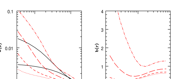
Figure 4: The angular cross correlation predictions for halos of masses $10^{10},10^{11},10^{12},10^{13}M_{\odot}$ (bottom to top), compared to the linear and PD predictions (solid curves).

Option (ii)—one and only galaxy per halo, and the galaxy sits at the halo centre—corresponds to setting $N_{\rm gal}(m)=1$ and $(2\pi)^{3}u_{\rm gal}(k|m)=1$ for all $m$ (we use $N_{\rm gal}(m)$ to denote $\langle N_{\rm gal}|m\rangle$ for simplicity). This is a reasonable model for the Large Red Galaxy (LRG) sample provided by the SDSS; results for this model are shown in Figure 4.

Option (iii) requires additional assumptions to fully specify the galaxy distribution. For example, one might expect the distribution of galaxies around the halo centre to depend on galaxy type. In what follows, we will assume for simplicity that the galaxies in a halo trace the dark matter: therefore, we set $u_{\rm gal}(k|m)=u(k|m)$. Sheth et al. (2001) show that this is a reasonable approximation. (See Scranton 2001 for more discussion of how $u_{\rm gal}$ might depend on galaxy type).

It is probably accurate to assume that one of the $N_{\rm gal}$ galaxies in a halo sits at the halo centre – this is almost certainly a good assumption if there is only one galaxy in a halo. To account for this, one assumes that the other galaxies get the usual density profile denoted by $u$, whereas the central galaxy is simply unity. To see the effect of this on the two-halo term, we must average both pieces of the two halo term over $p(n|m)$, the probability of having $n$ galaxies in a halo of mass $m$, with the requirement that $n>0$. With this averaging, we will replace $N_{\rm gal}(m)u_{\rm gal}(k|m)$ by an effective number of galaxies, $N_{\rm eff}$, which is a function of $k$ for given $m$. It is given by (Cooray & Sheth 2002)

$$N_{\rm eff}(k|m) \equiv \sum_{n>0}\ \left[1+(n-1)\ u(k|m)\right]\ p(n|m)$$ (9)

$$+ \sum_{n>0}\ \langle n-1|m\rangle\,u(k|m)+u(k|m)\,p(0|m).$$

The first term can be written as $[1-p(0|m)]$, allowing us to express the above equation as

$$N_{\rm eff}(k|m)=[1-p(0|m)]\,[1-u_{\rm gal}(k|m)]+\langle n|m\rangle\,u_{\rm gal}(k|m).$$ (10)

Since both factors in the first term are positive, there is an enhancement in power from always placing one galaxy at the halo centre. Since $u(k|m)$ decreases as $k$ increases, the enhancement in power is largest on small scales (large $k$). In sufficiently massive halos one might expect to have many galaxies, and so $p(0|m)\ll 1$. In this limit, the expression above becomes $1-u(k|m)+\langle n|m\rangle\,u(k|m)=1+\langle n-1|m\rangle\,u(k|m)$. On the other hand, if most halos have no galaxies, then $p(1|m)$ is probably much larger than all other $p(n|m)$ with $n\geq 2$. Then the leading order term in the sum above is $p(1|m)$. Since $\langle n|m\rangle\equiv\sum np(n|m)\approx p(1|m)$, we have that $N_{\rm eff}(k|m)\approx\langle n|m\rangle$. In this limit, only a fraction $\langle n|m\rangle\ll 1$ of the halos contain a galaxy, and the galaxy sits at the halo centre, so there is no factor of $u$.

The contribution of the galaxy counts to the one halo term of the galaxy–mass correlation function is similar. Using the expressions above yields

$$P_{\rm gm}^{\rm 1h}(k) = \int{\rm d}m\,n(m)\,{m\over\bar{\rho}}\,|u(k|m)|\,{N_{\rm eff}(k|m)\over\bar{n}_{\rm gal}}$$

$$P_{\rm gm}^{\rm 2h}(k) \approx P_{\rm lin}(k)\ \int{\rm d}m\,n(m)\,{m\over\bar{\rho}}\,b(m)\,u(k|m)\$$ (11)

$$\qquad\times\int{\rm d}m\,n(m)\,b(m)\,{N_{\rm eff}(k|m)\over\bar{n}_{\rm gal}}.$$

If the run of galaxies around the halo centre is not the same as of the dark matter, then one simply uses $u_{\rm gal}$ instead of $u$ in $N_{\rm eff}$. If the two-halo term usually does not dominate the power on small scales (this is almost always a good approximation), it is reasonable to ignore the enhancement in power associated with the central galaxy, and to simply set $N_{\rm eff}(k|m)\approx\langle n|m\rangle\,u_{\rm gal}(k|m)\approx\langle n|m\rangle$. The one-halo term requires knowledge of $p(0|m)$. Since $p(0|m)$ is usually unknown, some authors (e.g., Seljak 2000) interpolate between the two limits discussed earlier by setting $N_{\rm eff}=\langle n|m\rangle\,u(k|m)$ if $\langle n|m\rangle\geq 1$, and $N_{\rm eff}=\langle n|m\rangle$ if $\langle n|m\rangle<1$. It is worth noting that the one halo term of the galaxy–galaxy correlation function is only slightly more complicated, as shown in Cooray & Sheth (2002).

3.1 Halo model details

The halo model is specified by the mass function $n(m)$, bias $b(m)$ and the halo profile $u(k|m)$. For the first two functions we use (e.g. Cooray & Sheth 2002)

$$n(m,z)\,{\rm d}m = {\bar{\rho}\over m}\,\nu f(\nu)\,{{\rm d}\nu\over\nu},$$

$$\nu f(\nu) = A(p)\left(1+(q\nu)^{-p}\right)\,\left({q\nu\over 2\pi}\right)^{1/2}\,\exp\left(-{q\nu\over 2}\right);$$

$$b(m) = 1+{q\nu-1\over\delta_{\rm sc}(z)}+{2p/\delta_{\rm sc}(z)\over 1+(q\nu)^{p}},$$

$${\rm where}\quad\nu \equiv {\delta^{2}_{\rm sc}(z)\over\sigma^{2}(m)},$$ (12)

and $p\approx 0.3$, $A(p)=[1+2^{-p}\Gamma(1/2-p)/\sqrt{\pi}]^{-1}\approx 0.3222$, and $q\approx 0.75$ (Sheth & Tormen 1999). Here $\delta_{\rm sc}(z)$ is the critical density required for spherical collapse at $z$, extrapolated to the present time using linear theory, and

$$\sigma^{2}(m)={4\pi\over(2\pi)^{3}}\int_{0}^{\infty}{{\rm d}k\over k}\,k^{3}P_{\rm Lin}(k)\ W^{2}(kR_{0}),$$ (13)

where $W(x)=(3/x^{3})[\sin(x)-x\cos(x)]$ and $R_{0}=(3m/4\pi\bar{\rho})^{1/3}$. That is to say, $\sigma(m)$ is the rms value of the initial fluctuation field when it is smoothed with a tophat filter of comoving size $R_{0}$, extrapolated using linear theory to the present time. If $p=1/2$ and $q=1$, then $n(m)$ is the same as that first written down by Press & Schechter (1974), and $b(m)$ is the same as that given by Cole & Kaiser (1989) and Mo & White (1996).

In addition, we will assume that the halo profiles have the form given by Navarro, Frenk & White (1996), truncated at the virial radius $r_{\rm vir}$ which is defined by requiring that $m=4\pi/3r_{\rm vir}^{3}\bar{\rho}\,\Delta_{\rm vir}$. For spatially flat universes with $\Omega_{0}=(1,0.3)$ and $\Lambda=1-\Omega$, $\Delta_{\rm vir}=(178,340)$. The Fourier transform of the density run around a halo of mass $m$ is

$$u(k|m) = f(c)\ \Big{[}\sin\kappa\Big{(}{\rm Si}[\kappa(1+c)]-{\rm Si}(\kappa)\Big{)}$$ (14)

$$+ \cos\kappa\Big{(}{\rm Ci}[\kappa(1+c)]-{\rm Ci}(\kappa)\Big{)}-\frac{\sin(\kappa c)}{\kappa(1+c)}\Big{]},$$

where $f(c)=1/[\ln(1+c)-c/(1+c)]$, $\kappa\equiv kr_{\rm vir}/c$, ${\rm Si}(x)=\int_{0}^{x}{\rm d}t\,\sin(t)/t$ is the sine integral and ${\rm Ci}(x)=-\int_{x}^{\infty}{\rm d}t\,\cos(t)/t$ is the cosine integral function. The concentration parameter of the halos depends on halo mass; we use the parametrization of this dependence given by Bullock et al. (2001):

$$c(m)\approx 9\left({m\over m_{*}}\right)^{-0.13}.$$ (15)

3.2 Galaxy Model Details

Our model for the galaxy distribution is taken from the GIF N-body simulations of the $\Lambda$CDM model, coupled to a semi-analytic galaxy formation model (Kauffmann et al. 1999). Catalogs of galaxy positions, apparent and absolute magnitudes, colors and star-formation rates, at a range of redshifts, are available at http://www.mpa-garching.mpg.de/GIF/. From the catalogs at redshifts $z=0.06$, 0.13, 0.27, 0.35, 0.42, and 0.52 we selected apparent magnitude limited samples which satisfied $17<r^{*}<21$. At each redshift we then computed the first and second factorial moments of the number of galaxies as a function of halo mass. The parameters for the first moment are given in Table 1. These galaxies also form a surface defined by the first and second factorial moments as a function of halo mass and galaxy absolute magnitude which we can also integrate over given our apparent magnitude limits and a redshift (Scranton 2002).

In the GIF models, the mean number of galaxies in a halo $\langle n|m\rangle$ evolves little out to $z\sim 0.5$ if the galaxies have the same fixed rest-frame luminosity. Thus at fixed luminosity the evolution of galaxy clustering is driven by the evolution of the halo population. However, this means that at fixed apparent magnitude, the case in which we are most interested, $\langle n|m\rangle$ evolves more strongly. This is because only the most luminous galaxies from the higher redshift samples satisfy the apparent magnitude limit, and, in halos which host only one galaxy, there is a tight correlation between halo mass and galaxy luminosity. In principle, fits to $\langle n|m\rangle$ at fixed luminosity, along with the assumption that these relations do not evolve, allow one to estimate how $\langle n|m\rangle$ depends on redshift for the apparent magnitude limits we apply. In practice, we chose the more tedious but accurate method of making redshift dependent fits to the apparent magnitude $\langle n|m\rangle$ relation in the GIF model. The results are shown in Figure 1.

Table 1: Parameters which specify the mean number of galaxies in halos as a function of halo mass: $N_{\rm gal}(m)\equiv(m/M_{0})^{\alpha}+A\exp\left[-A_{0}\left(log_{10}(m)-M_{B}\right)^{2}\right]$. This Table gives the parameter values for the qso-galaxy case, with the foreground galaxies selected in the magnitude range $17<r^{\prime}<22$.

$z$	log $M_{0}/h^{-1}M_{\odot}$	$\alpha$	$A$	$A_{0}$	$M_{B}/\log\left(h^{-1}M_{\odot}\right)$
0.06	12.30	1.05	0.98	11.56	11.55
0.13	12.47	1.03	0.96	0.62	11.42
0.27	12.74	0.94	0.87	1.65	12.10
0.35	12.82	0.79	0.84	7.41	12.25
0.42	13.11	0.76	0.91	7.3	12.45
0.52	13.67	0.84	1.03	10.07	12.68

Table 2: $N_{\rm gal}(m)$ as in Table 1, but for the galaxy-galaxy case, with the foreground galaxies in the apparent magnitude range $17<r^{\prime}<21$.

$z$	log $M_{0}/h^{-1}M_{\odot}$	$\alpha$	$A$	$A_{0}$	$M_{B}/\log\left(h^{-1}M_{\odot}\right)$
0.06	12.26	0.9	1.0	2.0	11.75
0.13	12.48	0.9	1.0	4.0	11.75
0.27	13.0	0.9	1.0	4.0	12.75
0.35	13.48	0.9	1.0	6.0	12.75
0.42	14.0	0.9	1.0	8.0	12.75
0.52	14.3	0.9	0.2	8.0	12.75

Table 3: $N_{\rm gal}(m)$ as in Table 2, but for “red” foreground galaxies, defined by the criterion $g^{\prime}-r^{\prime}>0.65$. The functional form is $N_{\rm gal}(m)\equiv(m/M_{0})^{\alpha}\exp(-M_{1}/m)$.

$z$	log $M_{0}/h^{-1}M_{\odot}$	$\alpha$	log $M_{1}/h^{-1}M_{\odot}$
0.06	11.70	1.2	10.0
0.15	11.70	1.0	11.7
0.26	12.18	0.8	12.0
0.35	12.18	0.5	12.0
0.42	12.85	0.5	12.0
0.52	12.85	0.5	12.0

3.3 Lens and source redshift distributions

Magnification bias with galaxy-galaxy lensing should be detected with SDSS data and forthcoming datasets such as the CFHT Legacy survey. The SDSS photometric survey will provide of order 1 million foreground galaxies and 100 million background galaxies with photometric redshifts. The expected signal is sensitive to the mean redshifts of the foreground and source populations, but only at the 10% level or less to the shape of the distribution. Given that there is some freedom in the selection of the two populations with photometric redshifts, we have chosen simple distributions for our model predictions. For a CFHT Legacy survey kind of dataset, we choose the foreground population to be uniformly distributed over $0.2<z<0.5$ and the sources at $z=1$. For predictions for the SDSS survey, we choose a much closer foreground population with $0.1<z<0.2$, and the sources at $z=0.4$. We have checked that for a realistic, broad source redshift distribution with the same mean redshift, the signal would be lower by about $5$%.

Our expected distributions of galaxies and QSOs from an SDSS-like dataset for measurement of the QSO magnification bias are much more constrained than for the galaxy-galaxy lensing case. First, we expect that the efficiency of photometric selection of QSOs, while high compared to previous work, will force the use of spectroscopically-confirmed QSOs. This will result in approximately $10^{5}$ QSOs, down three orders of magnitude from the number of galaxies in the photometric sample. Hence we will need to maximize the number of objects in our distributions rather than restricting them to narrower, easier-to-model bands in redshift. For galaxies, this means going to a broad cut in apparent magnitude: $17<r^{\prime}<22$, for example. Using the luminosity function from the CNOC2 survey (Lin et al 1999), we can translate such an apparent magnitude cut in the SDSS filters into a redshift distribution (Dodelson et al 2002) well fit by a simple functional form:

$$\frac{dN}{dz}\propto z^{a}\exp\left[-\left(z/z_{0}\right)^{b}\right].$$ (16)

The QSO sample distribution is more complicated. Due to a combination of the QSO luminosity function and the evolution of QSO colors in the SDSS filters with redshift, the redshift distriubtion of QSOs from the main SDSS sample requires two functions of the form given in Equation 16, with an appropriate amplitude ($A$) for each to properly characterize the relative abundance of QSOs below $z=2$ and those above. Table 4 gives the parameters for the galaxy and QSO redshift distributions, with the normalization set to $A=1$ for the galaxy distribution. In addition to these smooth distributions, we impose a strict redshift cut of $z<0.8$ for the galaxy distribution and $z>1$ for the QSO distribution to avoid intrinsic clustering between the two samples.

Table 4: Parameters for redshift distribution functions of galaxies and QSOs of the form $dN/dz=Az^{a}\exp[-(z/z_{0})^{b}]$.

Object	$A$	$a$	$z_{0}$	$b$
Galaxies	$1$	$1.56$	$0.296$	$1.76$
Low-$z$ QSOs	$253.28$	$2.58$	$1.67$	$13.44$
High-$z$ QSOs	$6.5\times 10^{-4}$	9.13	3.35	18.37

4 Results

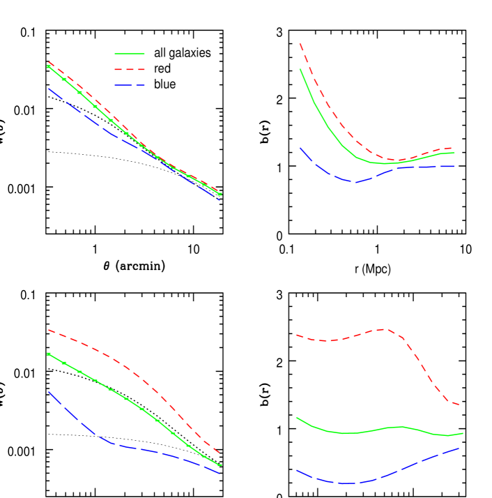
Figure 2: (i) The left panels show the angular cross correlation computed using the linear mass power spectrum (lower dotted curves), the nonlinear mass power spectrum (upper dotted), and three galaxy models (blue, total, red from bottom to top). The foreground galaxies are taken to lie between $0.2<z<0.5$ ($0.1<z<0.2$) and the sources at $z=1$ ($0.4$) for the upper (lower) panels. The error bars have been multiplied by 10 (see discussion in the text). (ii) The right panels show the ratio of the galaxy cross-correlations to the PD prediction. On large scales it is reasonable to interpret this ratio as a bias parameter, but on small scales it is important to consider the details of the halo occupation distribution of galaxies.

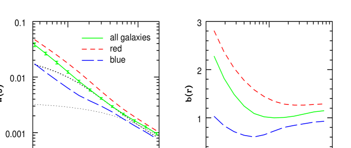
Figure 3: The angular cross correlation as in Figure 2, but for the qso-galaxy parameters appropriate for the SDSS survey.

Figures 2-4 show the predicted cross-correlation for different foreground-background populations. We use equation 6, with an $\Omega_{\rm m}=0.3,\Omega_{\lambda}=0.7$, $\Gamma=0.21$ cosmological model with $\sigma_{8}=0.8$ and the galaxy-mass power spectrum determined using the halo model ingredients described in Section 3. While $\sigma_{8}=0.8$ is close to the most recent determinations from the CMB and other datasets, there is uncertainty at about the 10% level in this parameter (e.g. Wang et al 2002; Spergel et al 2003; Verde et al 2003). Our results, especially for the higher redshift lens galaxies, are sensitive to $\sigma_{8}$: for higher $\sigma_{8}$, the lens galaxies are less biased and vice versa. Note that we have left out the $(2.5s-1)$ factor which depends on galaxy type. It will modulate both the amplitude and possibly the sign of our plotted cross-correlation.

We consider galaxy-galaxy correlations in Figure 2 for redshift distributions appropriate to the CFHT Legacy survey in the upper panels and the SDSS survey in the lower panel. The right panels show the ratio of the cross-correlation to the Peacock-Dodds prediction. On large scales this reduces to the usual bias parameter, but on small scales it must be interpreted more carefully in terms of properties of the halo occupation distribution. The results show that the cross-correlations are strongly dependent on galaxy-type and angular scale. This arises from the modeling of the “red” and “blue” galaxy sub-samples that make up the full foreground sample. The galaxy samples are defined by the $N_{\rm gal}(m)$ models given in Tables 2 and 3 for the full sample and for red galaxies (the blue galaxies are given by the difference of the two). Similar trends are seen in Figure 3, which uses the galaxy distribution in Table 4 and a mean redhisft $z=1.75$ for the quasars.

It is interesting that for red galaxies, lowering the redshifts of the source and lens population does not change the signal significantly (comparing the upper and lower panels of Figure 2). This is a consequence of how little $N_{\rm gal}(m)$ evolves between $z=0.5$ and $z=0$ for these galaxies. The net change in lensing signal as one lowers the redshifts is a trade off between two opposing effects: a reduction due to smaller lensing path length, and an increase because a given angle corresponds to a smaller length scale at the lens redshift. With a simplified power law model for the galaxy-mass power spectrum one can see that the net signal can increase with decreasing redshift. Let $P_{\rm gm}(k,a)\propto k^{-\alpha}a^{\beta}$, and let the lenses and sources be at a single redshift such that the distance to sources is twice the distance to the lenses. Then for an Einstein-de Sitter model equation 6 gives the analytic scaling

$$w(\theta)\propto a_{\rm lens}^{-{3\over 2}+{\alpha\over 2}+\beta}\ \theta^{2-\alpha}.$$ (17)

Thus for $\alpha=1$ (corresponding to a two-point correlation function with logarithmic slope of $-2$), one can see that $\beta>1$ would lead to an increasing signal with decreasing lens redshift. The choice $\alpha=1$ and $\beta=1$ is in good agreement with the behavior of the red galaxy sample, but not of the blue galaxies for which the cross-correlation is lower for lower redshifts of the lenses and sources. The differences between red and blue galaxies arise primarily from the difference in the $N_{\rm gal}(m)$ relation for them (Sheth et al 2001; Scranton 2002). On larger scales, corresponding to $r>1$Mpc, the difference between predictions for red and blue galaxies decreases. In the linear regime they are both expected to follow the growth rate of mass fluctuations, so the large-scale differences are primarily due to differences in $\alpha$.

We estimate the contribution of Poisson errors and sample variance on the measured $\omega(\theta)$. Scranton (2002) discusses the relative contributions of these errors and of the Gaussian and non-Gaussian terms in the covariance. Over the scales we have considered, the Poisson contribution dominates for a large survey like the SDSS. For parameters of the full SDSS survey, roughly 10 million galaxies in each sample and an area of 10,000 square degrees, the statistical errors are tiny. The errors are of order 1% of the signal and have been multiplied by a factor of 10 in Figure 2 to be visible at all. Clearly the signal to noise is high enough for such a dataset that estimates for sub-samples of galaxies by type and varying redshift bin are possible, thus allowing for the possibility of measuring their halo occupation properties in detail. The signal to noise can be scaled to other survey parameters relatively easily on small scales, where shot noise dominates so that the scaling is $\omega/\delta\omega\propto\sqrt{n_{1}n_{2}}\sqrt{\Omega}$, where $n_{1}$ and $n_{2}$ are the number densities of the two samples, and $\Omega$ is the survey area. Figure 3 shows that the errors expected from quasar-galaxy correlation measurements are significantly higher, due to the smaller number of quasars. Thus if systematic errors can be controlled, magnification bias is more effectly measured using galaxy-galaxy correlations.

The two major source of systematic errors are photometric calibration and errors in the photometric redshifts that are not well characterized or highly correlated with determination of the galaxy type. The latter leads to contamination of the samples: e.g. a foreground galaxy may be assigned to the background sample in the galaxy-galaxy case, or may in reality be physically associated with the quasar. In either case the auto-correlation signal, which is much stronger than the lensing signal, will get mixed in. Moessner & Jain (1998) estimate the required accuracy for photometric redshifts for a desired accuracy in the cross-correlation. Given the miniscule statistical errors, characterizing the systematic errors accurately will be paramount for any interpretation of results from either the CFHT or SDSS surveys.

For the quasar-galaxy $\omega(\theta)$ shown in Figure 3 the error bars are larger because of the smaller number of quasars compared to background galaxies. Even so, they are at the 1% level and would allow for a definitive measurement from the SDSS provided systematic errors are under control.

Figure 4 shows the cross-correlation for halos of different masses. This is not an observable, but it is helpful to see the wide variation in the signal as a function of halo mass since galaxies are modelled as occupying these halos. Clearly small changes in the $N_{\rm gal}(m)$ relation will change the expected signal since it will populate halos of different masses with galaxies differently. The dot-dashed curve shows the prediction for halos of mass $10^{13}M_{\odot}$, which have a very large amplitude at small scales. This is relevant for the SDSS since it will produce a sample of Large Red Galaxies, which are expected to occupy the centers of massive halos. A more quantitative connection is beyond the scope of this paper.

The redshift distribution of galaxies we have used has not been chosen to be consistent with the models for $N_{\rm gal}(m)$. This amounts to requiring from survey measurements that some (typically small) fraction of galaxies be discarded before estimating the cross-correlation to ensure consistency.

5 Discussion

We have used the halo model of clustering to estimate the cross-correlation induced by magnification bias between samples of galaxies and quasars at different redshifts. Our focus has been on the effect of the model for galaxies used on the predicted signal. We used fits to the GIF simulations for $N_{\rm gal}(m)$, the mean number of galaxies for halos of mass $m$, to find the number of galaxies as a function of redshift, magnitude and galaxy type. We find that the predicted cross-correlation is very sensitive to these parameters. Its amplitude varies on arcminute scales is a factor of 2 larger or smaller compared to an unbiased population, depending on the redshift range and galaxy type of the foreground population. The reason for this wide range is that on small scales the relation of the galaxy distribution to the mass is complex and cannot be described by a constant bias factor of order unity. Further, with increasing redshift a given apparent magnitude limit corresponds to brighter absolute magnitudes and therefore the selection of galaxies with higher $m/m_{*}$, which tend to be more strongly clustered. Our results on arcminute scales therefore differ from previous studies which used linear bias models.

The state of measurements of qso-galaxy correlations are summarized in Benítez et al (2001) and Guimaraes et al (2001). Clearly some of the measurements are affected by incomplete sampling and other observational systematics. Others find excess correlations on large scales, which are still difficult to reconcile with models. But most anomalous measurements are on arcminute scales where we find great sensitivity to the redshift distribution and galaxy type used for the measurement. Thus variations of a factor of 2 to even 10 in extreme cases can be explained. In existing data, the galaxy samples used are difficult to characterize given the lack of redhift or color information. The data discussed in Benítez & Martinez-Gonzalez (1995) show that the sample with red galaxies does have higher signal – this is consistent with our results, but it is difficult to be quantitative given the partial information available for the data.

In view of the massive improvement in the available sample expected from the SDSS and other forthcoming surveys such as the CFHT Legacy survey, we have chosen to simply provide model predictions for these surveys rather than attempt a detailed analysis of past measurements. Our models can be extended significantly, to include more detailed galaxy types and galaxy models that are checked for consistency with SDSS measurements of the galaxy auto-correlations.

The statistical errors expected from the SDSS survey are very small, about 1% of the signal for the full sample from galaxy-galaxy correlations. We have focused on scales below 20 arcminutes, where the signal to noise is high. On these scales the data from the SDSS can be split by galaxy type and redshift bins to make a detailed study of galaxy clustering in relation to the dark matter distribution. On large-scales the interpretation is simple, giving the bias parameter of desired galaxy sub-samples as a function of redshift.

What can we learn from sub-Mpc scale measurements of the galaxy-mass correlation? In the halo model, the 1-halo term is a linear measure of (the product of) $N_{\rm gal}(m)$ and other parameters: the halo mass function, halo mass profile and galaxy profile. Scranton (2002) analyzed the accuracy with which different parameters describing the galaxy distribution can be constrained using angular correlations from the photometric SDSS survey. Our results show that valuable additional information can be gained using measurements of magnification bias. In particular, the lensing induced cross-correlation is a measure of projected galaxy-mass correlations: it is thus linear in the parameters of the galaxy distribution such as the mean halo occupation number of galaxies $N_{\rm gal}(m)$. Galaxy clustering measurements probe the second moment of this distribution, and therefore one is required to make an assumption of how the second moment scales with the mean (on large scales galaxy clustering measurements do constrain the first moment through the two-halo term, but only averaged over a broad mass range). The magnification bias measurements considered here would constrain $N_{\rm gal}(m)$ directly and thus provide the basis for interpreting the higher order moments from galaxy clustering measurements. Further, the lensing measurement would help break the degeneracies between the various parameters.

Scranton (2002) gives the accuracy with which more than 10 parameter combinations will be constrained by SDSS measurements of the angular clustering of galaxies binned by photometric redshift. For the basic parameters of $N_{\rm gal}(m)$ in Table 1, he typically finds accuracies of well below 1%. For the lensing induced cross-correlation, the signal is significantly smaller and for the dominant parameters in $N_{\rm gal}(m)$ such as $\alpha$ one can expect better than 10% level accuracy from the lensing measurements alone. The main power however will be in combining the lensing and galaxy clustering measurements. We leave this exercise for future work.

Our formalism is similar to that of Seljak (2000) and Guzik & Seljak (2001) for galaxy-galaxy lensing. These authors have used measurements from the SDSS to constrain the mass profiles of large galaxy halos and the contribution of group halos (Guzik & Seljak 2002; see also McKay et al 2001). While in principal magnification bias measures a closely related cross-correlation (replacing the tangential shear with the convergence), in practice the measurements have been relevant on different scales. Galaxy-galaxy lensing has been measured so far on relatively small scales, the best signal being on $100-200$kpc. It remains to be seen from the completed SDSS survey and CFHT surveys how the relevant systematics play out for magnification and shear measures. It will be of great interest to analyze the measurements jointly to constrain galaxy-mass correlations. Similarly the large scale bias parameter inferred from shear surveys (Van Waerbeke 1998; Hoekstra et al 2002) can be directly compared with measurements of magnification bias. This will be an extremely useful cross-check since the errors in both measurements are likely to be dominated by systematic errors.

We have used the weak lensing approximation in this paper, setting $\mu=1+2\kappa$. There are corrections to this relation if $\kappa$ or $\gamma$ are of order unity (e.g. Ménard et al 2002). Correlations using the fully nonlinear magnification relation $\mu=1/[(1-\kappa)^{2}-\gamma^{2}]$ can be computed using the halo model approach developed in Takada & Jain (2003a,b). It leads to higher amplitudes for magnification bias on subarcminute scales, especially for source redshifts $\lower 2.15277pt\hbox{$\;\buildrel>\over{\sim}\;$}1$ (Takada & Hamana 2003); it will therefore be important to incorporate the nonlinear effects for deep surveys. Further, we have treated galaxies as points within halos, rather than subclumps with mass profiles. Using the formalism of Sheth & Jain (2002) we have estimated the effect and found it to be small for the range of scales studied in this paper.

We thank N. Benítez, A. Connolly, R. Scoccimarro, A. Szalay and M. Takada for helpful discussions. We thank the referee, Brice Ménard, whose comments helped improve and correct the paper. Some of the work presented here was begun during a summer 2002 workshop at the Aspen Center for Physics. BJ is supported by NASA grants NAG5-10923, NAG5-10924 and a Keck foundation grant.

Figure 1: The mean number of galaxies as a function of halo mass, $N_{\rm gal}(m)$, is shown for a range of redshifts. The symbols show the measurements from GIF simulations, and the solid curves shows our fits in Table 1.

References

- [] Bartelmann, M. 1995, A&A, 298, 661
- [Bartelmann & Schneider 1993a] Bartelmann, M. & Schneider, P. 1993, A&A, 268, 1
- [] Benítez, N., & Martinez-Gonzalez, 1995, ApJLett, 339, 53
- [] Benítez, N., & Martinez-Gonzalez, 1997, ApJ, 477, 27
- [] Benítez, N., Martinez-Gonzalez, E., Gonzalez-Serrano, J.I., & Cayon L. 1995, AJ, 109, 935
- [Benítez, Martinez-Gonzalez & Martin-Mirones 1997] Benítez, N., Martinez-Gonzalez, E. & Martin-Mirones, J. M. 1997, A&A, 321, L1
- [Benítez & Sanz 1999] Benítez, N. & Sanz, J. L. 1999, ApJLett, 525, L1
- [] Benítez, N., Sanz, J. & Martinez-Gonzalez, E., 2001, MNRAS, 320, 241
- [] Boyle, B.J., Fong, R. & Shanks, T. 1988, MNRAS, 231, 897
- [Bullock et al. 2001] Bullock, J. S., Kolatt, T. S., Sigad, Y., Somerville, R. S., Kravtsov, A. V., Klypin, A. A., Primack, J. R., Dekel, A., 2001, MNRAS, 321, 559
- [Canizares 1981] Canizares, C. R. 1981, Nature, 291, 620
- [] Cole, S., & Kaiser, N., 1989, MNRAS, 237, 1127
- [] Cooray, A., & Sheth, R., 2002, Phys. Rep., 372, 1
- [Croom & Shanks 1999] Croom, S. M. & Shanks, T. 1999, MNRAS, 307, L17
- [Dodelson et al. 2002] Dodelson, S. et al. 2002, ApJ, 572, 140
- [Dolag & Bartelmann 1997] Dolag, K. & Bartelmann, M. 1997, MNRAS, 291, 446
- [Drinkwater, Webster, Thomas & Millar 1992] Drinkwater, M. J., Webster, R. L., Thomas, P. A. & Millar, E. 1992, Proceedings of the Astronomical Society of Australia, 10, 8
- [Ferreras Benítez & Martinez-Gonzalez 1997] Ferreras, I. , Benítez, N. & Martinez-Gonzalez, E. 1997, AJ, 114, 1728
- [Fugmann 1988] Fugmann, W. 1988, A&A, 204, 73
- [] Fugmann, W. 1990, A&A, 240, 11
- [] Gaztanaga, E., 2003, ApJ, 589, 82
- [] Guimaraes, A., van De Bruck, C., Brandenberger, R., 2001, MNRAS, 325, 278
- [] Guzik, J, & Seljak, U., 2001, MNRAS, 321, 439
- [] Guzik, J, & Seljak, U., 2002, MNRAS, 335, 311
- [Hammer & Le Févre 1990] Hammer, F. & Le Févre, O. 1990, ApJ, 357, 38
- [] Hintzen, P., Romanishin, W., & Valdés, F., 1991, ApJ, 371, 49
- [] Hoekstra, H., et al, 2002, ApJ, 577, 604
- [1] Jain, B., & Seljak, U., 1997, ApJ, 484, 560
- [Jenkins et al. 1998] Jenkins, A., et al. 1998, ApJ, 499, 20
- [] Kauffmann, G., et al, 1999, MNRAS, 307, 529
- [Lin et al. 1999] Lin, H., Yee, H. K. C., Carlberg, R. G., Morris, S. L., Sawicki, M., Patton, D. R., Wirth, G., & Shepherd, C. W. 1999, ApJ, 518, 533
- [] McKay et al, 2001, astro-ph/0108013
- [] Ménard, B. & Bartelmann, M., 2002, A & Astrophys, 386, 784
- [] Ménard, B., Hamana, T., Bartelmann, M., & Yoshida, N., 2002, astro-ph/0210112
- [Mo & White 1996] Mo, H. J., White, S. D. M., 1996, MNRAS, 282, 347
- [Navarro, Frenk & White 1996] Navarro, J., Frenk, C., White, S. D. M., 1996, ApJ, 462, 563
- [2] Moessner, R., & Jain, B., 1998, MNRAS, 294, L18.
- [Norman & Impey 1999] Norman, D. J. & Impey, C. D. 1999, AJ, 118, 613
- [Norman & Williams 2000] Norman, D.J. & Williams, L.L.R. 2000, ApJ, 119, 2060
- [Norman & Impey 2001] Norman, D. J. & Impey, C. D. 2001, AJ, 121, 2392
- [Peacock 1982] Peacock, J. A. 1982, MNRAS, 199, 987
- [Peacock & Dodds 1996] Peacock, J. A. & Dodds, S. J. 1996, MNRAS, 280, L19
- [Peacock & Smith 2000] Peacock, J. A., Smith, R. E., 2000, MNRAS, 318, 1144
- [Press & Schechter 1974] Press, W., Schechter, P., 1974, ApJ, 187, 425
- [Rodrigues-Williams & Hogan 1994] Rodrigues-Williams, L. L. & Hogan, C. J. 1994, AJ, 107, 451
- [Romani & Maoz 1992] Romani, R. W. & Maoz, D. 1992, ApJ, 386, 36
- [Sanz, Marti nez-González & Benítez 1997] Sanz, J. L., Martinez-González, E. & Benítez, N. 1997, MNRAS, 291, 418
- [] Schneider, P., Ehlers, J., & Falco, E.E. 1992, Gravitational Lenses (Heidelberg: Springer)
- [Scoccimarro et al. 2001] Scoccimarro, R., Sheth, R. K., Hui, L., Jain, B., 2001, ApJ, 546, 652
- [] Scranton, R., 2003, MNRAS, 339, 410
- [] Seljak, U., 2000, MNRAS, 318, 203
- [Sheth & Tormen 1999] Sheth, R. K., Tormen, G., 1999, MNRAS, 308, 119
- [] Sheth, R. K., Jain, B., 2002, astro-ph/0208353
- [] Sheth, R., et al, 2001, MNRAS, 326, 463
- [] Spergel, D., et al, 2003, astro-ph/0302209
- [Takada & Jain 2003a] Takada, M. & Jain, B., 2003a, MNRAS, 340, 580
- [Takada & Jain 2003b] Takada, M. & Jain, B., 2003b, astro-ph/0304034
- [] Takada, M. & Hamana, T., 2003, astro-ph/0305381
- [] Thomas, P.A., Webster, R.L., & Drinkwater, M.J. 1994, MNRAS, 273, 1069
- [] Tyson, J.A., 1986, AJ, 92, 691
- [] Van Waerbeke, L., 1998, A & A, 331, 1
- [] Verde, L., et al, 2003, astro-ph/0302218
- [] Wang, X., et al, 2002, astro-ph/0212417
- [] Webster, R.L., Hewett, P.C., Harding, M.E., & Wegner, G.A. 1988, Nature, 336, 358
- [Williams & Irwin 1998] Williams, L. L. R. & Irwin, M. 1998, MNRAS, 298, 378
- [] Williams, L.L.R. 2000, ApJ, 535, 37