Assessment of the Fluorescence and Auger Data Base
used in Plasma Modeling

Abstract

We have investigated the accuracy of the $1s$-vacancy fluorescence data base of Kaastra & Mewe (1993) resulting from the initial atomic physics calculations and the subsequent scaling along isoelectronic sequences. In particular, we have focused on the relatively simple Be-like and F-like $1s$-vacancy sequences. We find that the earlier atomic physics calculations for the oscillator strengths and autoionization rates of singly-charged B II and Ne II are in sufficient agreement with our present calculations. However, the substantial charge dependence of these quantities along each isoelectronic sequence, the incorrect configuration averaging used for B II, and the neglect of spin-orbit effects (which become important at high-$Z$) all cast doubt on the reliability of the Kaastra & Mewe (1993) data for application to plasma modeling.

1 Introduction

In collisionally ionized or X-ray photoionized plasmas, high-energy electrons or photons lead to the production of $1s$-vacancy ionic states which then decay via sequential emission of single or multiple electrons and/or photons. The exact strengths of these competing processes determine fundamentally important quantities of the plasma such as the ionization balance and the observed spectra of emitted and/or absorbed photons. Hence, interpreting the properties of these plasmas requires accurate atomic physics calculations for the various autoionization and radiative rates. Here we are interested in assessing the accuracy of the available data base that provides such computed (or inferred) Auger rates and fluorescence yields to the astrophysics community. The accuracy of these atomic data are crucial to the interpretation of the spectra of photoionized plasmas such as are found in X-ray binaries and active galactic nuclei. These data are also important for supernova remnants (SNRs) under conditions of non-equilibrium ionization (NEI).

Two of the more widely used spectral codes for modeling photoionized plasmas are CLOUDY (Ferland et al., 1998) and XSTAR (Kallman & Bautista, 2001). A commonly used code for modeling NEI in SNRs is that of Borkowski, Lyerly, & Reynolds (2001). These all in turn rely on the table of electron and photon emission probabilities compiled by Kaastra & Mewe (1993). This comprehensive data base considers the sequential multiple electron and/or photon ejections for all stages of all $1s$-vacancy ions in the periodic table up through zinc. In order to produce such a massive array of numbers, however, certain approximations, questionable from a purely theoretical atomic physics standpoint, were invoked. First, the only rigorously computed atomic rates were taken from the early works of McGuire (1969, 1970, 1971, 1972) for singly-charged ions, which furthermore neglected configuration interaction (CI) and spin-orbit effects. Due to the limited computational resources available at the time, and the approximations thus needed to perform such calculations, even these cannot be considered as reliable as those that can be carried out with today’s state-of-the-art capabilities. Second, these singly-ionized results were then scaled along entire isoelectronic sequences, assuming constant autoionization rates and oscillator strengths; this approximation is least valid for near-neutrals.

A third approximation used by Kaastra & Mewe (1993) is that the electron and photon emission yields were computed using radiative and autoionization rates that were configuration averaged over possible terms, and the fluorescence yield was then given as a ratio of the averaged radiative rate to the sum of the averaged radiative and averaged Auger rate. For modeling purposes, however, this is incorrect; the actual required value is the average of the term-specific yields - an average of ratios rather than a ratio of averages. In other words, the relative probability of producing each specific inner-shell-vacancy term, and its subsequent term-specific decay, needs to be considered, and this was not done correctly for the data compiled by Kaastra & Mewe (1993) (see also Chen et al. (1985) for a further discussion of this importance).

In this paper, we investigate the validity of the above three approximations in order to assess the accuracy of the resultant data base of Kaastra & Mewe (1993). To this end, we first study the simplest $1s$-vacancy system that can radiate via a $2p\rightarrow 1s$ dipole-allowed transition. This is the removal of a $1s$ electron from the ground-state B-like sequence, or rather the $1s2s^{2}2p$ Be-like inner-shell excited sequence, which is investigated in the next section, and which is further simplified by the fact that only one electron, or one photon, can be emitted. We follow in Section 3 with a study of the simplest closed-(outer)shell case of F-like ions, corresponding to $1s$ vacancies from the Ne-like sequence. A summary of our findings and concluding remarks are then given in Section 4.

2 Case Study of the Be-Like Fluorescence Yields

Inner-shell $1s$ vacancy of a Be-like ion, whether by photoionization or electron-impact ionization of B-like ions (or by photoexcitation or electron-impact excitation of Be-like ions), results in either the $1s2s^{2}2p(^{1}P)$ state or the $1s2s^{2}2p(^{3}P)$ state. From an independent particle perspective, in LS coupling, the following competing decay processes can then occur:

$$1s2s^{2}2p(^{1}P) {A_{r}\atop\longrightarrow} 1s^{2}2s^{2}(^{1}S)+\omega\ ,$$ (1)

$$1s2s^{2}2p(^{1,3}P) {A_{a1}\atop\longrightarrow} 1s^{2}2s(^{2}S)\epsilon p(^{1,3}P)\ ,$$ (2)

$$1s2s^{2}2p(^{1,3}P) {A_{a2}\atop\longrightarrow} 1s^{2}2p(^{2}P)\epsilon s(^{1,3}P)\ ,$$ (3)

that is, the $1s$-vacancy state can either fluoresce, if it is in the ${}^{1}P$ state, with a radiative rate $A_{r}$, or autoionize, from either state, with a total state-dependent rate $A_{a}=A_{a1}+A_{a2}$, yielding free electrons denoted by $\epsilon l$. (If left in the ${}^{3}P$ state the ion does not fluoresce - we consider CI and spin-orbit effects in the next section). The radiative rate $A_{r}$ in atomic units (1 a.u. $=4.1341\times 10^{16}\ {\rm s}^{-1}$) is related to the dimensionless emission oscillator strength $f$ by

$$A_{r} = 2\omega^{2}\alpha^{3}f\ ,$$ (4)

where $\omega$ is the emitted photon energy in a.u. (1 a.u. of energy $=27.211$ eV) and $\alpha\approx 1/137$ is the fine structure constant. Here we define the emission oscillator strength as the absolute value of the oscillator strength from the upper $1s2s^{2}2p(^{1}P)$ term $j$ to the lower $1s^{2}2s^{2}(^{1}S)$ term $i$:

$$f \equiv \left|f_{ji}\right|\ ,$$ (5)

and can thus be related to the absorption oscillator strength $f_{ij}$ from the lower term $i$ to the upper term $j$ via

$$g_{i}f_{ij} = g_{j}\left|f_{ji}\right|\ ,$$ (6)

where $g_{i}=1$ and $g_{j}=3$ are the statistical weights of the initial and final Be-like terms, respectively.

Oscillator strengths are more convenient quantities to use along isoelectronic sequences because they exhibit certain bounds. Since the absorption oscillator strength is bounded by $0\leq f_{ij}\leq N_{i}$, where $N_{i}=2$ is the number of $1s$ electrons, the emission oscillator strength is bounded by $0\leq f\leq(g_{i}/g_{j})N_{i}=2/3$ (for the present cases), and is a well-behaved function of the nuclear charge $Z$. In fact, if the hydrogenic approximation is valid, i.e., if the nuclear potential dominates over the interelectronic repulsive potential, then the emission oscillator strength is independent of $Z$, and the same is true for the autoionization rate $A_{a}$. Such an approximation is valid for highly-charged ions but not for lower-charged species.

The fluorescence yield $\xi$, from a given inner-shell vacancy state, is a measure of the relative probabilities of the radiative and autoionization decay pathways and is defined as

$$\xi \equiv \frac{A_{r}}{A_{r}+A_{a}}=\frac{\omega^{2}}{\omega^{2}+\frac{1}{2\alpha^{3}}\left[\frac{A_{a}}{f}\right]}\ \ .$$ (7)

Thus it only depends on the squared transition energy $\omega^{2}$ and the ratio of the autoionization rate to the emission oscillator strength $A_{a}/f$. In the hydrogenic approximation, these scale respectively with nuclear charge as $q^{4}$ and $q^{0}$ (i.e., independent of $q$), where $q=Z-3$ is the asymptotic ionic charge seen by the outer-most electron of the Be-like ion (Cowan, 1981). With these scaling properties, the expected behaviors at low-$Z$ and high-$Z$ are $\xi\approx 0$ and $\xi\approx 1$ (provided $f\neq 0$), respectively.

2.1 Initial Populations, Configuration Interaction, and Spin-Orbit Effects

As pointed in Section 2, both the ${}^{1}P$ and ${}^{3}P$ terms can be populated after $1s$ photoionization or electron-impact ionization. Following Cowan (1981), and using the sudden approximation, we have determined that the probability of populating each term can be deduced by considering the squared recoupling coefficient

$$\left|\left\langle\left[\left(1s1s\right)\left({}^{1}S\right)\right]2p\left({}^{2}P\right)\left|\left[\left(1s2p\right)\left({}^{\left\{2{\cal S}+1\right\}}P\right)\right]1s\left({}^{2}P\right)\right\rangle\right|\right.^{2} = \left|\left(-1\right)^{1+{\cal S}}\left(2{\cal S}+1\right)^{\frac{1}{2}}\left\{\begin{array}[]{ccc}{\cal S}&\frac{1}{2}&\frac{1}{2}\\ 0&\frac{1}{2}&\frac{1}{2}\end{array}\right\}\right|^{2}$$ (10)

$$= \frac{2{\cal S}+1}{4}\ ,$$ (11)

where ${\cal S}=0$ for the ${}^{1}P$ state and ${\cal S}=1$ for the ${}^{3}P$ state. This means that the states are populated according to their statistical weights, and the ${}^{1}P$ state is populated with a probability of $1/4$. (In general, there also should be a recoupling coefficient involving the orbital angular momenta of the three electrons in Eq. 11; however, the $l=0$ values for two of the electrons’ orbital momenta reduces the coefficient to unity for the present case.) We have also verified this computationally by performing R-matrix photoionization calculations using the Wigner-Eisenbud R-matrix method (Burke & Berrington, 1993; Berrington et al., 1995). Using both approaches we find that in intermediate coupling, the states are also populated according to their statistical weights (a similar expression to Eq. 11 involving the total angular momentum values $j$ for each electron can be obtained).

Considering the relative populations of the $1s2s^{2}2p$ $1s$-vacancy states, the desired quantity for plasma modeling purposes is the configuration-average fluorescence yield. If CI and spin-orbit effects are neglected, this can be defined as an average over LS single-configuration (SC) terms as

$$\xi_{LSSC} \equiv \frac{1}{4}\xi{(^{1}P)}+\frac{3}{4}\xi{(^{3}P)}$$ (12)

$$= \frac{1}{4}\xi{(^{1}P)}$$

$${\longrightarrow\atop z\rightarrow\infty} \frac{1}{4}\ ,$$

where fluorescence from the ${}^{3}P$ state is zero so that the asymptotic behavior at large $Z$ is $1/4$.

CI and spin-orbit effects modify this behavior, however. The largest CI effect is the intrashell mixing $c_{1}1s2s^{2}2p+c_{2}1s2p^{3}$, where the mixing fraction $|c_{2}/c_{1}|^{2}$ is essentially term independent and $Z$ independent for nonrelativistic calculations - it varies between 0.067 for B II and 0.053 for Zn XXVII. This mixing affects the computed emission oscillator strength $f$ and autoionization rate $A_{a}$ at the near neutral end of the sequence, but changes the high-$Z$ fluorescence yield by less than 10%. The more important CI effect is that the admixture of the $1s2p^{3}$ configuration in the ${}^{3}P$ term allows it to radiate to the $1s^{2}2p^{2}(^{3}P)$ state. This $c_{2}1s2p^{3}(^{3}P)\rightarrow 1s^{2}2p^{2}(^{3}P)$ radiative rate is about a factor of 20 smaller than the $1s2s^{2}2p(^{1}P)\rightarrow 1s^{2}2s^{2}(^{1}S)$ rate, so it only increases the fluorescence yield by a few percent at low $Z$. As $Z$ increases, however, eventually even this reduced radiative rate dominates the autoionization rate, giving

$$\xi_{LSCI} \equiv \frac{1}{4}\xi{(^{1}P)}+\frac{3}{4}\xi{(^{3}P)}$$ (13)

$${\longrightarrow\atop z\rightarrow\infty} 1\ .$$

The spin-orbit interaction also affects the computed fluorescence yield, primarily by mixing the ${}^{1}P_{1}$ and ${}^{3}P_{1}$ levels. The mixing fraction, while only about $6.3\times 10^{-6}$ at $Z=5$, has a $Z^{4}$ dependence, and eventually becomes quite significant, reaching $0.117$ at $Z=30$. As a result, the “${}^{3}P_{1}$” level (this is now just a label used to indicate the dominant term of a level) has an increased fluorescence yield, and we get that the intermediate coupling (IC), configuration-averaged fluorescence yield, including CI, behaves as

$$\xi_{ICCI} \equiv \frac{3}{12}\xi{(^{1}P_{1})}+\frac{1}{12}\xi{(^{3}P_{0})}+\frac{3}{12}\xi{(^{3}P_{1})}+\frac{5}{12}\xi{(^{3}P_{2})}$$ (14)

$$\geq \xi_{LSCI}\ .$$

Thus we see that CI and the spin-orbit interaction each cause an increase in the computed fluorescence yield as $Z$ is increased.

2.2 Earlier Be-like Fluorescence Data

The approach of Kaastra & Mewe (1993) for this particular Be-like series was to neglect spin-orbit and CI effects, and to assume that the hydrogenic approximation is valid throughout the series. Furthermore, they used configuration-averaged values for the B II autoionization rate and emission oscillator strength, which were computed by McGuire (1969), and the experimental values of $\omega$ from Lotz (1967, 1968), to obtain the ratio $A_{r}/(A_{r}+A_{a})$ required for determining $\xi$ using Eq. 7. This is not the same as the desired configuration-averaged fluorescence yield $\xi_{LSSC}$ in Eq. 12 - the ratio of the averages does not equal the average of the ratios:

$${\sum_{{\cal S}=0,1}({2{\cal S}+1\over 4})A_{r}(^{2{\cal S}+1}P)\over\sum_{{\cal S}=0,1}({2{\cal S}+1\over 4})\left[A_{r}(^{2{\cal S}+1}P)+A_{a}(^{2{\cal S}+1}P)\right]} \neq \sum_{{\cal S}=0,1}\left({2{\cal S}+1\over 4}\right)\left[{A_{r}(^{2{\cal S}+1}P)\over A_{r}(^{2{\cal S}+1}P)+A_{a}(^{2{\cal S}+1}P)}\right]\ .$$ (15)

We first address the accuracy of the computed autoionization rates and emission oscillator strengths in the next subsection, and then address the validity of the hydrogenic approximation in the following subsection. Fluorescence yields are presented in the last subsection, where the incorrect averaging and neglect of CI and spin-orbit effects by Kaastra & Mewe (1993) are addressed.

2.3 Atomic Calculations for B II

In order to calculate the transition matrix elements appearing in the expressions for the radiative and autoionization rates (Cowan, 1981), it is first necessary to produce atomic wave functions. McGuire (1969) used the Herman-Skillman approximation in determining the (single-configuration) wave functions, whereby all electrons (i.e., the $1s$, $2s$, $2p$, and continuum ones) are eigenfunctions of a common central potential; as stated by McGuire (1969), this “neglect(s) … exchange and correlation effects.” Furthermore, this potential $rV(r)$ is approximated by “a series of straight lines” in order to yield piece-by-piece analytic Whitakker functions. Here we are concerned with the validity of these approximations, given that more rigorous calculations can be easily performed using today’s state-of-the-art technologies.

For the present study, we use the program AUTOSTRUCTURE (Badnell, 1986), which generates Slater-type $1s$, $2s$, $2p$, and distorted-wave continuum orbitals. In order to compare with the results of McGuire (1969) for B II, and with Kaastra & Mewe (1993) as we scale from $Z=5$ to $Z=30$, we first performed single-configuration LS calculations. For the more rigorous calculations that we compare to other theoretical results and that we recommend as the definitive data, we also included CI - $1s2s^{2}2p\ +\ 1s2p^{3}$ for the inner-shell vacancy state and $1s^{2}2s^{2}\ +\ 1s^{2}2p^{2}$ for the final radiative decay state - and spin-orbit effects. The two accessible continua were described as $1s^{2}2s\epsilon p$ and $1s^{2}2p\epsilon s$, where $\epsilon l$ denotes a continuum distorted wave.

Given atomic wave functions, McGuire (1969) computed the configuration average (CA) radiative and partial autoionization rates in Eqs. 1-3. The emission oscillator strength given is thus

$$f(CA) = \frac{1}{4}f(^{1}P)+\frac{3}{4}f(^{3}P)$$ (16)

$$= \frac{1}{4}f(^{1}P)$$

$$= 0.0377\ ,$$

whereas for the total autoionization rate, the CA rates for the processes in Eqs. 2-3 were used, that is,

$$A_{a}(CA) = A_{a1}(CA)+A_{a2}(CA)$$ (17)

$$= 2.37\times 10^{-3}\ {\rm a.u.}\ ,$$

where

$$A_{a1}(CA) = \frac{1}{4}A_{a1}(^{1}P)+\frac{3}{4}A_{a1}(^{3}P)$$ (18)

$$= \frac{1}{4}\left\{2\pi\left[R_{0}(1s,\epsilon p,2s,2p)-\frac{2}{3}R_{1}(1s,\epsilon p,2p,2s)\right]^{2}\right\}$$

$$+\frac{3}{4}\left\{2\pi\left[R_{0}(1s,\epsilon p,2s,2p)\right]^{2}\right\}\ .$$

and

$$A_{a2}(CA) = \frac{1}{4}A_{a2}(^{1}P)+\frac{3}{4}A_{a2}(^{3}P)$$ (19)

$$= 2\pi\left[R_{0}(1s,\epsilon s,2s,2s)\right]^{2}\ ,$$

since our calculations indicate that $A_{a2}(^{1}P)=A_{a2}(^{3}P)$. Here $R_{\lambda}(n_{1}l_{1},n_{2}l_{2},n_{3}l_{3},n_{4}l_{4})$ is a Slater integral of multipole $\lambda$ (Cowan, 1981), and $\epsilon l$ represents the outgoing $l$-wave continuum electron orbital. (The expressions in Eqs. 18 and 19 are equivalent to those in Eq. 6 of McGuire (1969) for inequivalent electrons and single-$p$ orbital occupation, considering the different continuum normalization used by McGuire (1967)). Note that the partial rate $A_{a1}(^{1}P)$ in Eq. 18 is greatly suppressed relative to the $A_{a1}(^{3}P)$ rate due to a near cancellation of monopole and dipole Slater integrals. (Indeed, it was due to this near cancellation of Slater integrals that Caldwell et al. (1990) explained why the inner-shell photoexcited $1s2s^{2}2p(^{1}P)$ resonance in Be I preferentially decayed - by two orders of magnitude - to the $1s^{2}2p(^{2}P)+e^{-}$ channel, compared to the $1s^{2}2s(^{2}S)+e^{-}$ channel.) Thus the configuration average partial rate $A_{a1}(CA)$ will be larger than the partial rate $A_{a1}(^{1}P)$, and hence the configuration average total rate $A_{a}(CA)$ will be larger than $A_{a}(^{1}P)$.

Since we are interested in computing $\xi(^{1}P)$, which requires $A_{a}(^{1}P)$ and $f(^{1}P)$, we have converted the reported values from McGuire (1969) to the ${}^{1}P$ values (the Slater integrals were also given in that work). We get the following values

$$f(^{1}P,{\rm McGuire}) = 0.1508$$ (20)

$$A_{a}(^{1}P,{\rm McGuire}) = 1.692\times 10^{-3}\ {\rm a.u.}\ ,$$ (21)

which compare fairly well with our results obtained using AUTOSTRUCTURE:

$$f(^{1}P,{\rm present}) = 0.1519$$ (22)

$$A_{a}(^{1}P,{\rm present}) = 1.045\times 10^{-3}\ {\rm a.u.}$$ (23)

In summary, we find that the earlier results for B II of McGuire (1969) are consistent with ours. However, for the astrophysical plasma modeling purposes we have in mind, one really requires the configuration average fluorescence yield, not the ratio of the averaged radiative and total rates used by Kaastra & Mewe (1993)

$$\xi(K\&M) = \frac{A_{r}(CA)}{A_{r}(CA)+A_{a}(CA)}$$ (24)

$${\longrightarrow\atop z\rightarrow\infty} 1\ ,$$

due to $A_{r}$ and $A_{a}$ scaling as $q^{4}$ and $q^{0}$, respectively, in the hydrogenic approximation. Equation 24 differs from the correct $\xi_{LSSC}$ given in Eq. 12. First, we have $A_{a}(CA)>A_{a}(^{1}P)$ due to the near cancellation in the ${}^{1}P$ $2s2p\rightarrow 1s\epsilon p$ partial autoionization rate, so at low $Z$, where $A_{r}\ll A_{a}$, we have $\xi(K\&M)<\xi_{LSSC}$. Second, when CI and spin-orbit effects are ignored, as they were in Kaastra & Mewe (1993), the fluorescence yields differ asymptotically by a factor of 4,

$$\lim_{Z\rightarrow\infty}\frac{\xi(K\&M)}{\xi_{LSSC}} = 4\ ,$$ (25)

as can be seen by comparing Eqs. 12 and 24. Of course, CI needs to be included for all $Z$, whereas spin-orbit mixing needs to be included at higher $Z$, and both $\xi(K\&M)\rightarrow 1$ and $\xi_{ICCI}\rightarrow 1$ as $Z\rightarrow\infty$. However, in the intermediate $Z$ range, it can be shown that the Kaastra & Mewe (1993) results are still larger than the ICCI results.

2.4 Validity of the Hydrogenic Approximation

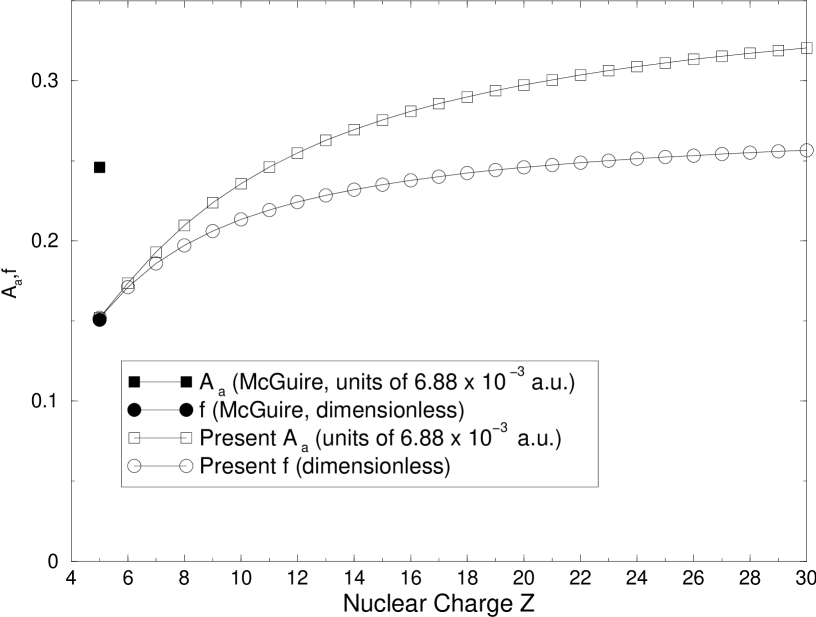
Figure 1: Present LS autoionization rates $A_{a}$ (in units of $6.88\times 10^{-3}$ a.u., open squares) and emission oscillator strengths $f$ (dimensionless, open circles) for Be-like $1s2s^{2}2p(^{1}P)$ ions as a function of the nuclear charge $Z$. The autoionization rate and emission oscillator strength from McGuire (1969) for B II are shown by the solid square and circle, respectively.

In order to assess the validity of scaling the B II results along the isoelectronic series, we computed both the ${}^{1}P$ autoionization rate $A_{a}$ and emission oscillator strength $f$ for all Be-like ions up through zinc, first neglecting spin-orbit effects. In Fig. 1, it is seen that neither of the two is independent of the nuclear charge $Z$ at the lowest stages of ionization - the emission oscillator strength increases by about $2/3$ in going toward the highly-ionized regime whereas the autoionization rate more than doubles. Furthermore, by choosing the scale so that our two quantities coincide for B II, it is seen that the important ratio $A_{a}/f$ appearing in Eq. 7 increases by roughly 25% by the time Zn XXVII is reached. Thus the assumption of pure hydrogenic scaling by Kaastra & Mewe (1993) alone introduces an uncertainty at the highly-charged end of this series. Due to the stronger $Z$ dependence at the near-neutral end, together with the greater sensitivity to the atomic basis used in this region, we recommend that if scaling along an isoelectronic sequence is to be performed, the better starting point would be at the highest $Z$ desired, extrapolating the rates to lower $Z$ members. Of course, given the ease of determining atomic rates with modern computing capabilities, the most reliable approach is to calculate the fluorescence yield directly rather than resort to questionable scaling methods.

2.5 Fluorescence Yield Results

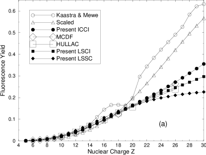
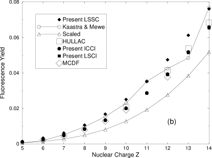
Figure 2: (a) Comparison of various computed and inferred fluorescence yields $\xi$ for Be-like $1s2s^{2}2p$ ions: present LS results in the single-configuration (SC) approximation – solid diamonds; present LS results with configuration interaction (CI) included – solid squares; present intermediate coupling (IC) results with CI included – solid circles; HULLAC results from Behar & Netzer (2002) – open squares; MCDF results from Chen (1985) – open diamonds; Kaastra & Mewe (1993) – open circles; results when we scale McGuire (1969) B II results, using Eq. 7 and the $\omega$ from Lotz (1967, 1968) – open triangles. (b) Same as (a) focusing on the low-$Z$ region.

While the assumption of hydrogenic scaling introduces an $\approx 25\%$ inaccuracy in $A_{a}/f$, the initial quantity being scaled in Kaastra & Mewe (1993) - the ratio of averages rather than the average of ratios - is really not the desired quantity to be scaled in the first place. Together, these approximations lead to an uncertain prediction for the fluorescence yield. In Fig. 2 (and Table 1), we compare various results for $\xi$ along the Be-like sequence, where it can be seen that our single-configuration LS results differ greatly from those of Kaastra & Mewe (1993), especially at higher $Z$; here, especially, their results are expected to differ from the correct single-configuration values due to their incorrect asymptotic value given by Eq. 24. A more disturbing result was found when we tried to repeat their calculations, i.e., when we used Eq. 7, with the ratio of $A_{a}(CA)/f(CA)$ taken from McGuire (1969), and the energies $\omega$ taken from Lotz (1967, 1968). Whereas these scaled results exhibit a smooth monotonic increase with nuclear charge $Z$, those of Kaastra & Mewe (1993) are somewhat irregular, showing unphysical dips, and do not agree with what we tried to reproduce, given their stated method. Either way, the results of Kaastra & Mewe (1993), or our scaled ones using the B II results of McGuire (1969), initially underestimate our results at lower $Z$, and then overestimate our (LSSC) results by almost a factor of 3 for the highest $Z=30$.

To our knowledge, there have been two other calculations for the fluorescence yields of some members of the Be-like sequence: those of Behar & Netzer (2002) using the HULLAC codes (Bar-Shalom et al., 2001) and those of Chen (1985) using a multiconfiguration Dirac-Fock (MCDF) method. In both cases, CI and spin-orbit effects were included. Here we do the same, first adding the important $2s^{2}\rightarrow 2p^{2}$ CI discussed earlier to the LS calculations in order to see that this effect increases the $Z=30$ fluorescence yield by about 30%. Then when spin-orbit effects (and other higher-order, relativistic effects) are included in our intermediate coupling calculation, there is a further increase in the fluorescence yield by about 20% more. In comparison with the other two calculations along this series, there is overall good agreement with these IC results.

3 Case Study of the F-Like Fluorescence Yields

We turn now to the simplest closed-(outer)shell case of a $1s$-vacancy in F-like ions, giving the $1s2s^{2}2p^{6}(^{2}S)$ state which decays as

$$1s2s^{2}2p^{6}(^{2}S) {A_{r}\atop\longrightarrow} 1s^{2}2s^{2}2p^{5}(^{2}P)+\omega$$ (26)

$${A_{a}\atop\longrightarrow} \left\{\begin{array}[]{l}1s^{2}2p^{6}(^{1}S)\epsilon s\\ 1s^{2}2s2p^{5}(^{1,3}P)\epsilon p\\ 1s^{2}2s^{2}2p^{4}(^{3}P,\,^{1}D,\,^{1}S)\epsilon s,\epsilon d\end{array}\right.\ .$$ (30)

Again, only one photon, or one electron, can be emitted, which simplifies the analysis considerably (when spin-orbit effects are considered, the final ionic term in Eq. 26 is fine structure split into the ground $1s^{2}2s^{2}2p^{5}(^{2}P_{3/2})$ level and the metastable $1s^{2}2s^{2}2p^{5}(^{2}P_{1/2})$ level). Since this is a closed-shell system, the Herman-Skillman method for the important $2p$ electrons is expected to be more accurate than for B II. Indeed, as stated by McGuire (1969), “in stripping away electrons (in reducing to a closed-shell system), … we should be increasing the applicability of the common central-field approximation.” Furthermore, there is only one $1s2s^{2}2p^{6}$ $1s$-vacancy state, rather than the two we had for the Be-like sequence, and no other intrashell configurations to CI mix with, so we do not need to consider population of non-fluorescing states by CI or spin-orbit mixing, nor do we have to consider configuration averaging issues. Consequently, a single configuration LS coupling calculation is sufficient to determine accurate $A_{a}$, $f$, and $\xi$ values for the ${}^{2}P$ term.

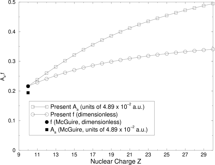
Figure 3: Present LS emission oscillator strengths $f$ (dimensionless, open circles) and autoionization rates $A_{a}$ (in units of $4.89\times 10^{-2}$ a.u., open squares) for F-like $1s2s^{2}2p^{6}(^{2}S)$ ions as a function of the nuclear charge $Z$. The emission oscillator strength and autoionization rate from McGuire (1969) for Ne II, as used by Kaastra & Mewe (1993), are shown by the solid circle and square, respectively.

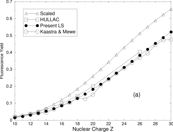
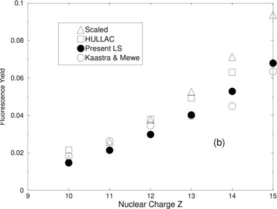
Figure 4: (a) Comparison of various computed and inferred fluorescence yields $\xi$ for F-like $1s2s^{2}2p^{6}(^{2}S)$ ions: present LS results – solid circles; Kaastra & Mewe (1993) – open circles; results when we scale McGuire (1969) Ne II results using Eq. 7 and the $\omega$ from Lotz (1967, 1968) – open triangles; HULLAC results of Behar & Netzer (2002) – open squares. (b) Same as (a) focusing on the low-$Z$ region.

As a result, the computed values of the autoionization rate and emission oscillator strength given by McGuire (1969) agree quite well with our values, as seen in Fig. 3 and Table 2. However, both of these values depend on the internuclear charge $Z$, giving a ratio $A_{a}/f$ that increases by about a factor of $1/2$ in going from Ne II to Zn XXII. Thus the scaled fluorescence yield $\xi$, using Eq. 7, the ratio $A_{a}/f$ from McGuire (1969), and $\omega$ from Lotz (1967, 1968), increases relative to the actual computed value, as is seen in Fig. 4 and Table 2. The more troublesome news in this figure is the actual tabulated values of Kaastra & Mewe (1993) - their values do not follow our attempt at reproducing those results, but rather tend to follow our computed values, except for certain unphysical dips. Nevertheless, the results reported by Kaastra & Mewe (1993) for F-like ions are not plagued by as many uncertainties as those for Be-like ions. We also see in Fig. 4 that the HULLAC results are in good agreement with our present ones (the results reported earlier by Behar & Netzer (2002) only considered fluorescence into the $1s^{2}2s^{2}2p^{5}(^{2}P_{3/2})$ level, which includes only 4 of all 6 magnetic sublevels of the $1s^{2}2s^{2}2p^{5}(^{2}P)$ configuration; therefore, those values must be multiplied by about 3/2 to account for fluorescence into the two $1s^{2}2s^{2}2p^{5}(^{2}P_{1/2})$ sublevels as well. Furthermore, the earlier HULLAC result for F⁺ was erroneously listed incorrectly, and here we have given the actual computed value that should have appeared).

4 Summary and Conclusion

The inaccuracies we have discovered in the reported results of Kaastra & Mewe (1993) for Be-like ions are as follows:

1. The computed atomic data for B II are used in the form $A_{a}(CA)/f(CA)$, that is, the radiative and autoionization rates have been averaged over the ${}^{1}P$ and ${}^{3}P$ configurations, whereas the desired quantity for plasma modeling applications is $\xi_{ICCI}$ and is not the same thing, differing qualitatively and quantitatively, especially in the asymptotic high-$Z$ limit.

2. The hydrogenic scaling assumed is invalid. The autoionization rates, the emission oscillator strengths, and even the ratio $A_{a}/f$ are not independent of nuclear charge $Z$.

3. The tabulated data of Kaastra & Mewe (1993) do not seem to follow the results we obtain when we try to reproduce their stated method using Eq. 7, with $A_{a}(CA)/f(CA)$ from McGuire (1969), and $\omega$ from Lotz (1967, 1968).

4. The calculations of Kaastra & Mewe (1993) neglected CI and spin-orbit effects as they scaled to higher $Z$.

For F-like ions, items 1 and 4 are not issues since there is only one inner-shell vacancy term. However, points 2 and 3 still apply for the F-like sequence. For plasma modeling purposes, we recommend our $\xi_{ICCI}$ for the Be-like sequence and our $\xi$ for the F-like sequence.

In conclusion, we propose that, given the many uncertainties discovered, the entire data base of Kaastra & Mewe (1993) should be reevaluated. While we have focused on systems that can emit only one photon or one electron, their comprehensive tabulation also includes data for ions with $n\geq 3$ shells occupied; these can emit multiple electrons and/or photons through numerous cascading channels, compounding the inaccuracies we have discovered.

Table 1: Emission oscillator strengths, autoionization rates, fluorescence yields, and photon energies for Be-like $1s2s^{2}2p$ ions.

$Z$	$f$	$A_{a}$	$\xi$	$\xi$	$\omega$	$\xi$	$\xi$	$\xi$	$\xi$	$\xi$
	present	present	present LSSC	K&M	Lotz	Scaled	HULLAC	MCDF	present LSCI	present ICCI
5	0.1519	0.1045	0.0014	0.0006	6.751	0.0006			0.0011	0.0011
	0.1508	0.1692
6	0.1712	0.1194	0.0032	0.0019	10.349	0.0013		0.0024	0.0025	0.0025
7	0.1859	0.1328	0.0061	0.0052	14.721	0.0027		0.0045	0.0048	0.0048
8	0.1972	0.1442	0.0106	0.0096	19.866	0.0049		0.0079	0.0083	0.0083
9	0.2062	0.1540	0.0168	0.0154	25.753	0.0081		0.0128	0.0132	0.0133
10	0.2134	0.1622	0.0250	0.0229	32.379	0.0128	0.0209	0.0191	0.0199	0.0201
11	0.2193	0.1693	0.0352	0.0352	39.782	0.0192			0.0285	0.0287
12	0.2243	0.1754	0.0474	0.0424	47.924	0.0276	0.0414	0.0377	0.0390	0.0393
13	0.2285	0.1808	0.0612	0.0484	56.806	0.0384	0.0538		0.0514	0.0518
14	0.2320	0.1854	0.0761	0.0768	66.465	0.0518	0.0685		0.0653	0.0658
15	0.2351	0.1896	0.0916	0.1102	76.862	0.0681			0.0805	0.0812
16	0.2378	0.1933	0.1073	0.1446	88.034	0.0874	0.0984		0.0965	0.0974
17	0.2402	0.1965	0.1225	0.1656	99.982	0.1100			0.1129	0.1141
18	0.2423	0.1995	0.1369	0.1671	112.664	0.1357	0.1273	0.1237	0.1295	0.1309
19	0.2442	0.2022	0.1502	0.1626	126.122	0.1644			0.1458	0.1478
20	0.2459	0.2046	0.1623	0.1984	140.348	0.1958	0.1569		0.1616	0.1646
21	0.2475	0.2068	0.1732	0.2963	155.342	0.2298			0.1769	0.1813
22	0.2488	0.2089	0.1828	0.3438	171.107	0.2658			0.1916	0.1982
23	0.2501	0.2108	0.1912	0.3838	187.645	0.3033			0.2058	0.2154
24	0.2513	0.2125	0.1985	0.4214	204.991	0.3419			0.2194	0.2333
25	0.2523	0.2141	0.2049	0.4562	223.108	0.3810			0.2327	0.2518
26	0.2533	0.2156	0.2105	0.4903	241.998	0.4200	0.2394	0.2633	0.2457	0.2713
27	0.2542	0.2169	0.2153	0.5267	261.659	0.4584			0.2585	0.2916
28	0.2551	0.2182	0.2194	0.5836	282.129	0.4960			0.2712	0.3125
29	0.2559	0.2194	0.2230	0.6215	303.333	0.5322			0.2840	0.3339
30	0.2566	0.2205	0.2261	0.6322	325.310	0.5668			0.2969	0.3553

Table 2: Emission oscillator strengths, autoionization rates, fluorescence yields, and photon energies for F-like $1s2s^{2}2p^{6}(^{2}S)$ ions.

$Z$	$f$	$A_{a}$	$\xi$	$\xi$	$\omega$	$\xi$	$\xi$
	present	present	present	K&M	Lotz	Scaled	HULLAC
10	0.2159	0.1056	0.0147	0.0182	31.184	0.0169	0.0215
	0.216	0.0948
11	0.2286	0.1164	0.0214	0.0263	38.723	0.0258
12	0.2406	0.1273	0.0298	0.0346	47.035	0.0376	0.0380
13	0.2515	0.1377	0.0402	0.0397	56.081	0.0526	0.0493
14	0.2615	0.1477	0.0528	0.0449	65.864	0.0712	0.0630
15	0.2705	0.1571	0.0679	0.0634	76.422	0.0936
16	0.2786	0.1659	0.0855	0.0875	87.720	0.1197	0.0983
17	0.2859	0.1741	0.1058	0.1019	99.795	0.1497
18	0.2926	0.1817	0.1286	0.1305	112.646	0.1832	0.1443
19	0.2987	0.1888	0.1540	0.1253	126.276	0.2199
20	0.3042	0.1954	0.1818	0.1505	140.682	0.2592	0.2001
21	0.3093	0.2016	0.2118	0.2073	155.863	0.3004
22	0.3139	0.2073	0.2437	0.2411	171.820	0.3429
23	0.3182	0.2127	0.2771	0.2751	188.552	0.3860
24	0.3221	0.2177	0.3116	0.3068	206.093	0.4289
25	0.3258	0.2224	0.3469	0.3386	224.395	0.4710
26	0.3291	0.2269	0.3825	0.3692	243.504	0.5118	0.4041
27	0.3324	0.2309	0.4180	0.3942	263.386	0.5513
28	0.3353	0.2348	0.4531	0.4438	284.040	0.5883
29	0.3380	0.2385	0.4874	0.4734	305.465	0.6230
30	0.3406	0.2420	0.5207	0.4758	327.735	0.6554

References

- Badnell (1986) Badnell, N. R. 1986, J. Phys. B, 19, 3827
- Bar-Shalom et al. (2001) Bar-Shalom, A., Klapisch, M., & Oreg, J. 2001, J. Quant. Spectr. Radiat. Transfer, 71, 169
- Behar & Netzer (2002) Behar, E., & Netzer, H. 2002, ApJ, 570, 165
- Berrington et al. (1995) Berrington, K.A., Eissner, W. B., & Norrington, P. H. 1995, Comput. Phys. Commun., 92, 290
- Borkowski, Lyerly, & Reynolds (2001) Borkowski, K. T., Lyerly, W. J., & Reynolds, S. P. 2001, ApJ, 548, 820
- Burke & Berrington (1993) Burke, P. G., & Berrington, K. A. 1993, Atomic and Molecular Processes: An R-matrix Approach, (IOP Publishing, Bristol)
- Caldwell et al. (1990) Caldwell, C. D., Flemming, M. G., Krause, M. O., van der Meulen, P., Pan, C., & Starace, A. F. 1990, Phys. Rev. A, 41, 542
- Chen et al. (1985) Chen, M. H., Craseman, B., & Matthews, D. L. 1985, Phys. Rev. Lett., 34, 1309
- Chen (1985) Chen, M. H. 1985, Phys. Rev. A, 31, 1449
- Cowan (1981) Cowan, R. D. 1981, The Theory of Atomic Structure and Spectra, (University of California, Berkeley).
- Ferland et al. (1998) Ferland, G. J., Korista, K. T., Verner, D. A., Ferguson, J. W., Kingdon, J. B., & Verner, E. M. 1998, PASP, 110, 761
- Froese Fischer (1991) Froese Fischer, C. 1991, Comput. Phys. Commun., 64, 369
- Kaastra & Mewe (1993) Kaastra, J. S., & Mewe, R. 1993, A&AS, 97, 443
- Kallman & Bautista (2001) Kallman, T. R., & Bautista, M. 2001, ApJS, 133, 221
- Lotz (1967) Lotz, W. 1967, J. Opt. Soc. Am., 57, 873
- Lotz (1968) Lotz, W. 1968, J. Opt. Soc. Am., 58, 915
- McGuire (1967) McGuire, E. J. 1967, Phys. Rev., 161, 51
- McGuire (1969) McGuire, E. J. 1969, Phys. Rev., 185, 1
- McGuire (1970) McGuire, E. J. 1970, Phys. Rev. A, 2, 273
- McGuire (1971) McGuire, E. J. 1971, Phys. Rev. A, 3, 587
- McGuire (1972) McGuire, E. J. 1972, Phys. Rev. A, 5, 1052