2-point anisotropies in WMAP and the Cosmic Quadrupole

Abstract

Large-scale modes in the temperature anisotropy power spectrum $C_{l}$ measured by the Wilkinson Microwave Anisotropy Probe (WMAP), seem to have lower amplitudes ($C_{2}$, $C_{3}$ and $C_{4}$) than that expected in the so called concordance $\Lambda$CDM model. In particular, the quadrupole $C_{2}$ is reported to have a smaller value than allowed by cosmic variance. This has been interpreted as a possible indication of new physics. In this paper we re-analyse the WMAP data using the 2-point angular correlation and its higher-order moments. This method, which requires a full covariance analysis, is more direct and provides better sampling of the largest modes than the standard harmonic decomposition. We show that the WMAP data is in good agreement ($\simeq 30\%$ probability) with a $\Lambda$CDM model when the WMAP data is considered as a particular realization drawn from a set of realistic $\Lambda$CDM simulations with the corresponding covariance. This is also true for the higher-order moments, shown here up to 6th order, which are consistent with the Gaussian hypothesis. The sky mask plays a major role in assessing the significance of these agreements. We recover the best fit model for the low-order multipoles based on the 2-point correlation with different assumptions for the covariance. Assuming that the observations are a fair sample of the true model, we find $C_{2}=123\pm 233$, $C_{3}=217\pm 241$ and $C_{4}=212\pm 162$ (in $\mu K^{2}$). The errors increase by about a factor of 5 if we assume the $\Lambda$CDM model. If we exclude the Galactic plane $|b|<30$ from our analysis, we recover very similar values within the errors (ie $C_{2}=172,C_{3}=89,C_{4}=129$). This indicates that the Galactic plane is not responsible for the lack of large-scale power in the WMAP data.

1 Introduction

Measurements of the cosmic microwave background (CMB) anisotropies by WMAP (Bennett et al. 2003; Spergel et al. 2003; Peiris et al. 2003) are in good agreement with a ‘concordance’ cosmology based on the $\Lambda$CDM model. However, the WMAP results also confirm the low amplitude of the CMB quadrupole first measured by COBE (eg Hinshaw et al. 1996a). As Bennett et al. (2003) comment, the amplitudes of the quadrupole and the octopole are low compared with the predictions of $\Lambda$CDM models. The WMAP team also present a convincing case that the low CMB multipoles are not significantly affected by foreground Galactic emission (see also Tegmark, de Oliveira-Costa and Hamilton 2003). The discrepancy between the observations and the $\Lambda$CDM model is particularly evident in the temperature angular correlation function, which shows an almost complete lack of signal on angular scales $\lower 2.15277pt\hbox{$\;\buildrel>\over{\sim}\;$}60$ degrees. According to Spergel et al. (2003), the probability of finding such a result in a spatially-flat $\Lambda$CDM cosmology is about $1.5\times 10^{-3}$. This is small enough to require an explanation, e.g. in the form of new physics Contaldi et al. (2003) or in terms of spatial curvature Efstathiou 2003a .

In this paper we consider the WMAP data from the point of view of the two-point angular correlation function as opposed to the usual harmonic decomposition. In some aspects our approach is similar to the study presented by Hinshaw et al. (1996b) for the COBE data. The paper is organized as follows. In §2 we introduce our methodology and test it with realistic simulations. In §3 we apply our method to the real WMAP data and present a comparison with the simulations. We also describe the application of higher-order statistics to test the Gaussianity of WMAP. The conclusions are described in §4.

2 2-pt correlation $w_{2}(\theta)$ in $\Lambda$CDM models

On the largest scales, the 2-point correlation $w_{2}(\theta)$ has some important advantages and disadvantages over spherical harmonics. The overall shape of the 2-point function is very sensitive to small differences in power at low multipoles. This is clearly an advantage when measuring the quadrupole. On the other hand, different bins in $\theta$ are highly correlated, which means that we need to use the full covariance matrix to assess the significance of any departures between measurements and models. Another important advantage of using the 2-point function is that large-scale modes can be easily sampled from any region of the sky, even when a mask is required, provided the region is large enough. In comparison, harmonic decomposition breaks the angular symmetry in the sky into orthogonal bases which have an arbitrary phase orientation. This is not a problem in the case of full sky coverage, but the results will be coordinate-dependent if a mask is used. Moreover, the harmonic coefficients $a_{lm}$ (see Eq.3) over masked data are convolved with the harmonic image of the mask. The resulting coupling matrix needs to be inverted and the resulting estimator for the recovered coefficients is typically biased because of the non-linear transformations involved. These potential complications are avoided in configuration space.

2.1 Definition and estimators

The 2-point angular correlation function is defined as the expectation value or mean cross-correlation of density fluctuations at two positions ${\bf q}_{1}$ and ${\bf q}_{2}$ in the sky:

$$\mbox{$$}w_{2}(\theta)\equiv\langle\Delta T({\bf{\bf q}_{1}})\Delta T({\bf{\bf q}_{2}})\rangle,$$ (1)

where $\theta=|\bf{{\bf q}_{2}}-\bf{{\bf q}_{1}}|$, assuming that the distribution is statistically isotropic.

To estimate $w_{2}(\theta)$ from the pixel maps we use a simple but effective estimator:

$$\mbox{$$}w_{2}(\theta)={\sum_{i,j}\Delta_{i}\Delta_{j}~{}w_{i}~{}w_{j}\over{\sum_{i,j}w_{i}~{}w_{j}}},$$ (2)

where $\Delta_{i}$ and $\Delta_{j}$ are the temperature differences in the map and the sum extends to all pairs separated by $\theta\pm\Delta\theta$. The differences are normalised so that $\langle\Delta_{i}\rangle=0$. The weights $w_{i}$ can be used to minimise the variance when the pixel noise is not uniform, but this introduces larger cosmic variance. Here we follow the WMAP team and use uniform weights (i.e. $w_{i}=1$). We use bins $\Delta\theta$ whose size is proportional to the square root of the angle $\theta$.

This estimator is unbiased and is equivalent to the minimum variance estimator of Landy & Szalay (1993). For higher-order moments see §3.6.

2.2 The $\Lambda$CDM Model and simulations

Temperature fluctuations can be expanded in terms of spherical harmonics according to,

$$\mbox{$$}\Delta T({\bf q})=\sum_{\ell=0}^{\infty}\sum_{m=-\ell}^{\ell}a_{\ell m}Y_{\ell}^{m}({\bf q}),$$ (3)

which defines the multipole power spectrum: $C_{l}=<|a_{\ell m}|^{2}>$. Gaussian simulations can then be made by taking $a_{\ell m}$ to be independent Gaussian fields with random phases, zero mean and variance $C_{l}$.

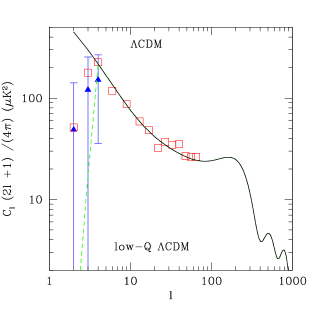
In order to test the significance of the correlations measured in the WMAP data, we make simulated sky maps by using the best-fit cosmological parameters estimated from WMAP (Spergel et al. 2003). The theoretical power spectra are generated using the publicly available CMBFAST package (Seljak & Zaldarriaga 1996). The $C_{l}$s are normalised to the COBE spectra and the input parameters are listed in Table 1. Along with cosmological parameters, CMBFAST accepts a reionization optical depth, $\tau$, and the scalar spectral index, $\eta_{s}$. From now on we refer to this particular set of paramenters as the $\Lambda$CDM model. Figure 1 shows the resulting power spectrum for the $\Lambda$CDM model. In the $\Lambda$CDM model the first three non-zero multipoles are (in $\mu K^{2}$):

$$\mbox{$$}C_{2}=1130,\ \ C_{3}=537,\ \ C_{4}=304,$$ (4)

while Bennett et al. (2003) find from WMAP data:

$$\mbox{$$}C_{2} = 129\pm 799$$

$$C_{3} = 320\pm 320$$

$$C_{4} = 316\pm 104.$$ (5)

Table 1: CMBFast Cosmological Parameters

Parameter	Value
H0	72 km/s/Mpc
$\Omega_{b}$	.046
$\Omega_{c}$	.224
$\Omega_{\Lambda}$	.730
$\Omega_{k}$	0.0
$\tau$	.17
$\eta_{s}$	1.0

Figure 1: Power spectrum $C_{l}$ for the $\Lambda$CDM model (continuous line). Open squares show the first multipoles by Bennett et al. (2003). Closed triangles with errors correspond to Eq.[3.5]. Unlike the conventional way of plotting this curve, each amplitude here shows the contribution of each multipole to the sky anisotropies in Eq. [7]. Dashed line shows the low-Q model in Eq. [6].

This power spectrum is then used as input to generate all-sky CMB maps using the HEALPix package (Górski, Hivon & Wandelt 1999). We simulate 100 V-band maps (FWHM = 21’ at 61 GHz), each with a different random phase, using the best fit WMAP power spectra These maps are all generated with the RING pixelization scheme and nside=512. Noise is added to the simulations following the pixel-noise pattern in the WMAP data. We also impose the most conservative WMAP kp0 foreground mask to the simulations.

For some crucial aspects of the analysis we have used an additional set of 2000 V-band $\Lambda$CDM simulations to check how the results depend on the number of simulations used. In general we find that with 20 simulations one finds similar qualitative conclusions to those with 2000 simulations, with a typical uncertainty of $\simeq 50\%$ in the intervals of confidence (see below §3.4).

2.3 The low-Q $\Lambda$CDM model

As a useful comparison model, we design a fiducial variation of the $\Lambda$CDM model with low values of the quadrupole and octopole. This new model is identical to the $\Lambda$CDM model for $l>3$ but has zero quadrupole $C_{2}=0$ and half the octopole $C_{3}\rightarrow C_{3}/2$. As we will show later, this model is in better agreement with the WMAP data than the $\Lambda$CDM model and follows the curved universe with a truncated spectrum Efstathiou 2003a . Thus, we modify the $\Lambda$CDM power spectrum by setting:

$$\mbox{$$}C_{2}^{low-Q} = 0$$ (6)

$$C_{3}^{low-Q} = \frac{1}{2}C_{3}^{\Lambda CDM}$$

$$C_{l}^{low-Q} = C_{l}^{\Lambda CDM},\ l>3.$$

We refer to this model as low-Q $\Lambda$CDM . These new $C_{l}$’s are then used to generate 20 HEALPix V-band maps, each with a different random phases.

2.4 Predicted $w_{2}(\theta)$ from $C_{l}$

The 2-pt function, $w_{2}(\theta)$, is the Fourier transform of the angular power spectrum of temperature fluctuations. In terms of the $C_{l}$ in Eq. [3], we have (see e.g. Bond & Efstathiou 1987):

$$\mbox{$$}w_{2}(\theta)={1\over{4\pi}}\sum_{l=2}~{}(2l+1)~{}C_{l}~{}P_{l}(\cos{\theta}),$$ (7)

where $P_{l}$ are the Legendre polynomials. The sum starts at $l=2$ because the monopole and the dipole have been subtracted from the WMAP data (CMB rest frame).

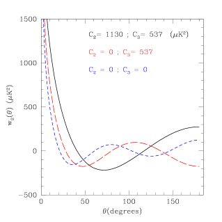
Figure 1 shows the multipole coefficients for the $\Lambda$CDM and low-Q models. Figure 2 shows the corresponding analytical summation for all multipoles $l\geq 2$ (continuous line), $l\geq 3$ (long-dashed line) and $l\geq 4$ (short-dashed line). The figure very clearly illustrates the sensitivity of the angular 2-point function to the low multipoles: e.g. varying just the quadrupole completely changes the shape of the curve at large scales.

Figure 2: Theoretical prediction of the 2-point angular correlation $w_{2}$ in the $\Lambda$CDM model with all multipoles (continuous line), without the quadrupole (long dashed line) and without quadrupole and octopole (short dashed line).

2.5 $w_{2}(\theta)$ from simulations

Figure 3 compares the theoretical values of $w_{2}(\theta)$ in the $\Lambda$CDM and low-Q models with that estimated from the simulated maps. The continuous line is the mean of the different realizations of each model and the dashed line is the theoretical estimate corresponding to the set of $C_{l}$s. The shaded area shows the 1-sigma dispersion of the simulations in each bin. As can be seen from the figure, the $\Lambda$CDM model has the larger errors. This is expected since the $\Lambda$CDM model has stronger lower-order multipoles which in turn lead to larger variations from realization to realization.

Figure 3: The 2-pt function $w_{2}(\theta)$ from simulations (continuous line) with 1-sigma confidence region (shaded region) compared to $w_{2}(\theta)$ from the input $C_{l}$ spectrum (dashed line). Top left: $\Lambda$CDM model with kp0-mask. Top right: $\Lambda$CDM model with kp0-mask and $|b|>30$ Galactic cut. Bottom left: low-Q model with kp0-mask. Bottom right: low-Q model with kp0-mask and $|b|>30$ Galactic cut.

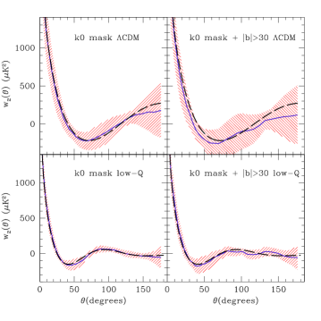
The right-hand panels in Figure 3 show the estimation of $w_{2}$ for pixels within Galactic latitudes $|b|>30$ degrees. This reduces the number of pixels by almost a factor of two which results in larger errors. Note how the recovered values of $w_{2}$ are not strongly biased within the error bars. Thus, even after excluding a broad Galactic region one can still use $w_{2}$ to separate a low and high quadrupole in the data. We will further elaborate on this point later in the paper.

2.6 Error bars

The absolute error (1-sigma dispersion) as a function of scale from different realizations of each model is shown in Figure 4. As can be seen from the figure, errors for the $\Lambda$CDM simulations (long-dashed lines) are much larger than errors in the low-Q model (short-dashed line). Note also how the low-Q model estimation is more noisy since it is based on 20 realizations, while there are 100 and 1000 realizations in the $\Lambda$CDM model.

Figure 4: Short, long-dashed and dotted lines show the absolute errors (or dispersion) in $w_{2}$ from the low-Q simulations, the first 40 and the first 1000 $\Lambda$CDM simulations respectively. The continuous lines corresponds to estimated jackknife errors with N=8 and N=32 subsamples within the WMAP data, while the shaded region shows the dispersion in jackknife errors from each of the low-Q realizations.

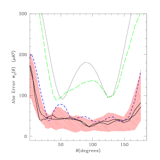
The shaded region represents the dispersion (2-sigma) in the jackknife errors (see below) for the different low-Q realizations.

2.7 Covariance Matrix

As mentioned before there is strong covariance between different bins in $w_{2}(\theta)$. This is mostly due to the fact that the lowest $l$ multipoles, and therefore larger scales, have more power than higher $l$ multipoles (e.g. see Fig. 1). As $w_{2}(\theta)$ is dominated by large scale modes, the correlations at different scales are strongly correlated. This is obviously worse in the $\Lambda$CDM model than in the low-Q $\Lambda$CDM , which has a lower quadrupole and octopole.

It is therefore essential that we estimate the covariance between different bins in $w_{2}(\theta)$. This can be calculated from the simulations by using the following definition of the covariance matrix:

$$\mbox{$$}C_{ij} \equiv \langle\Delta w_{2}(\theta_{i})~{}\Delta w_{2}(\theta_{j})\rangle$$ (8)

$$= {1\over{N}}\sum_{L=1}^{N}\Delta w_{2}^{L}(\theta_{i})\Delta w_{2}^{L}(\theta_{j}),$$

where

$$\mbox{$$}\Delta w_{2}^{L}(\theta_{i})\equiv w_{2}^{L}(\theta_{i})-\widehat{w_{2}}(\theta_{i}).$$ (9)

Here $w_{2}^{L}(\theta_{i})$ is the 2-point function measured in the $L$-th realization ($L=1\dots N$) and $\widehat{w_{2}}(\theta_{i})$ is the mean value for the $N$ realizations. The case $i=j$ gives the error variance: $\sigma_{i}^{2}\equiv C_{ii}$.

It is also useful to define the normalised covariance matrix (or correlation matrix), as:

$$\mbox{$$}\widetilde{C_{ij}}\equiv{C_{ij}\over{\sqrt{C_{ii}{C_{jj}}}}}$$ (10)

Figure 5: Normalised covariance (or correlation) matrices between different angular bins in $w_{2}(\theta)$ . Grey scale goes from -1 (black) to +1 (white). Left: $\Lambda$CDM model. Middle: low-Q model. Right: jackknife samples in low-Q model.

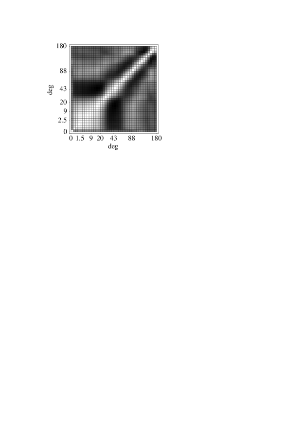
Figure 5 shows the normalised covariance in the $\Lambda$CDM (left) and low-Q model (middle). The covariance shown for the $\Lambda$CDM model corresponds to 40 realizations, but very similar pictures are obtained for a 1000 realizations. The covariance matrix is quite different in these two cases as the $\Lambda$CDM model shows correlations on larger scales because of the higher quadrupole and octopole. Note in particular the strong anticorrelation between angular bins in the range 50-100 degrees with the bins on larger and smaller scales. This is clearly an indication of very large variations in the low order multipoles within different realizations (eg see Fig.2). Note also how the errors in the first bin (zero-lag in $w_{2}$) is dominated by instrumental noise so that this bin is not correlated with the rest of the bins (grey color corresponds to zero).

2.8 Jackknife covariance

We can also estimate the errors in $w_{2}(\theta)$ from a single simulation, or from the real sky with a variation of the jackknife error scheme proposed by Scranton et al. (2001). This has the potential advantage of producing an error estimate which is model independent. In the estimation, the sample is first divided into $M$ separate regions on the sky, each of equal area. The analysis is then performed $M$ times, on each occasion removing a different region. These are called the (jackknife) subsamples, which we label $k=1\dots M$. The estimated statistical covariance for $w_{2}$ at scales $\theta_{i}$ and $\theta_{j}$ is then given by:

$$\mbox{$$}C_{ij} = {M-1\over{M}}\sum_{k=1}^{M}\Delta w_{2}^{k}(\theta_{i})\Delta w_{2}^{k}(\theta_{j})$$ (12)

$$\Delta w_{2}^{k}(\theta_{i})\equiv w_{2}^{k}(\theta_{i})-\widetilde{w_{2}}(\theta_{i})$$

where $w_{2}^{k}(\theta_{i})$ is the measure in the $k$-th subsample ($k=1\dots M$) and $\widetilde{w_{2}}(\theta_{i})$ is the mean value for the $M$ subsamples. The case $i=j$ gives the error variance. Note how, if we increase the number of regions $M$, the jackknife subsamples are larger and each term in the sum is smaller. We typically take $M=16$ corresponding to dividing the sphere into 8 octants and each octant in two (by longitude). We have checked that the resulting covariance gives a stable answer for different choices of shapes and $M$ from $M=8$ to $M=32$.

The mean normalised jackknife covariance shown in the right panel of Fig. 5 is in very good agreement with the sample covariance shown in the middle panel. The jackknife covariance appears smoother because it is the mean of 20x16 jackknife samples, while the sample covariance is the mean of only 20 samples. Other than this, the jackknife matrix correctly captures all the relevant correlation information present in the ensemble. The corresponding diagonal errors are shown in Fig. 4.

In general, one would not expect such a good agreement, because the jackknife method can not account for variations on scales larger than the jackknife samples. In our case, however, by construction there is little power on the largest scales (quadrupole and octopole) in the low-Q model. This explains the good performance of the jackknife method.

2.9 $\chi^{2}$ test

In order to quantify how well a model fits the data we use a $\chi^{2}$ test. Since the bins of the $w_{2}(\theta)$ are correlated, however, the simple $\chi^{2}$-test is not valid but must be modified by using the covariance matrix. The value of the $\chi^{2}$ is given by

$$\mbox{$$}\chi^{2}=\sum_{i,j=1}^{N}\Delta_{i}~{}C_{ij}^{-1}~{}\Delta_{j},$$ (13)

where $\Delta_{i}\equiv w_{2}^{O}(\theta_{i})-w_{2}^{M}(\theta_{i})$ is the difference between the ”observation” $O$ and the model $M$. In terms of the reduced covariance matrix, this is

$$\mbox{$$}\chi^{2}=\sum_{i,j=1}^{N}\Big{(}{\Delta_{i}\over\sigma_{i}}\Big{)}~{}\widetilde{C}_{ij}^{-1}~{}\Big{(}{\Delta_{j}\over\sigma_{j}}\Big{)}.$$ (14)

2.10 Singular Value Decomposition

In using real world data, one must worry about degeneracies in the covariance matrix due to an over-determined system and noise. If the rows (or columns) of $C_{ij}$ are not independent, the determinant of the matrix is zero and there is no inverse. With real data, the determinant of $C_{ij}$ will not typically be zero but the matrix can have very small eigenvalues which then lead to artificially large eigenvalues of the inverse matrix.

In order to eliminate the degeneracies in the covariance matrix, we perform a Singular Value Decomposition (SVD) of the matrix,

$$\mbox{$$}\widetilde{C_{ij}}=(U_{ik})^{\dagger}W_{kl}V_{lj},$$ (15)

where $W_{kl}$ is a diagonal matrix with the singular values on the diagonal. By doing the decomposition, we can choose the number of modes we wish to include in our $\chi^{2}$ by effectively setting the corresponding inverses of the small singular values to zero.

In practice we find that the SVD is only required when we use a small number of simulations to estimate the covariance matrix. With more than 100 simulations we find that the covariance matrix inversion is stable and one then gets more accurate $\chi^{2}$ values.

2.11 Recovering $C_{l}$ from $w_{2}(\theta)$

Using the SVD of the covariance matrix we can recover $C_{l}$s from $w_{2}(\theta)$ by requiring a minimum $\chi^{2}$ (see Szapudi et al. 2001 for a different approach). To test the method, we have recovered the low $C_{l}$s from the $\Lambda$CDM and low-Q modes. These are shown in Figures Fig. 6 and Fig. 7 respectively. The confidence contours are plotted relative to the minimum $\chi^{2}$ value.

Figure 6: Recovered values of $(C_{2},C_{3})$ (upper panel) and $(C_{2},C_{4})$ (lower panel) from the $\Lambda$CDM model. The black box indicates the values used to generate $w_{2}(\theta)$ and the gray box the recovered value. Confidence contours are plotted at 10, 68 and 98% of the minimum $\chi^{2}$ value.

Figure 7: Recovered values of $(C_{2},C_{3})$ (upper panel) and $(C_{2},C_{4})$ (lower panel) from the low-Q model. The black box indicates the values used to generate $w_{2}(\theta)$ and the gray box the recovered value. Confidence contours are plotted at 10, 68 and 98% of the minimum $\chi^{2}$ value.

As it is clear from the figures, the method accurately reproduces the correct values of the $C_{l}$s. We have also checked that this method is robust and insensitive to the number of modes used in the calculation.

3 Results from WMAP

3.1 Estimation of $w_{2}(\theta)$ in WMAP

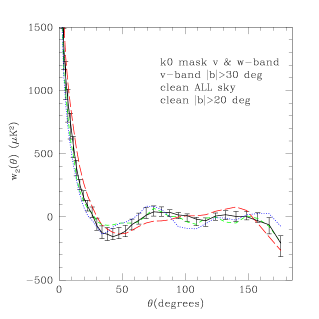
Figure 8 shows different estimations of $w_{2}(\theta)$ from the WMAP data. These different estimates gives an idea of the systematics involved, which are related mostly to possible Galactic and foreground contamination in the maps (see Bennet et al. 2003, Tegmark et al. 2003 for more details). Also note how the jackknife errors (from the dispersion in the V-band estimates from different regions in the sky) roughly include the variations in these different estimations. Thus we will use V-band estimates with jackknife errors as representative of WMAP sampling variance and systematic uncertanties.

Note how our estimates of $w_{2}(\theta)$ agree well with that presented by the WMAP collaboration (e.g. compare to Fig.13 in Bennett et al. 2003).

Figure 8: Error bars represent the 2-point angular correlation and 1-sigma jackknife dispersion $w_{2}$ in the WMAP V-band. The continuous line, passing through the error-bars, shows $w_{2}$ in the WMAP W-band. These two cases have the kp0 mask, while the dotted line excludes all the Galactic plane with $b>30$ deg. The long and short dashed lines correspond to the foreground clean map of Tegmark etal (2003) with and without a Galactic cut $|b|>20$.

3.2 Comparison of $w_{2}(\theta)$ to simulations

Figure 9: The 2-point angular correlation $w_{2}$ in the WMAP V-band data (points with jackknife error bars) compared to the $\Lambda$CDM simulations (shaded region corresponds to 1-sigma error dispersion). In both cases we use the kp0 Galactic mask.

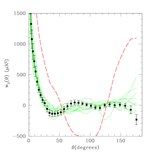
Figure 9 compares the WMAP $w_{2}(\theta)$ estimation with the 1-sigma dispersion in the corresponding $\Lambda$CDM simulations. At first sight one might conclude that a $\Lambda$CDM model is ruled out to a high significance. It should be remembered, however, that there is a strong covariance in the $w_{2}(\theta)$ estimation (see Fig.5). This point is illustrated in Figure 10 which shows 10 of the $\Lambda$CDM realizations that happens to have a low quadrupole and are compared with one that happen to have a high quadrupole (all chosen from the first 100 $\Lambda$CDM simulations). Note how systematics effects in WMAP (which are well represented by the jackknife errors) are comparable to the differences between these 10 $\Lambda$CDM simulations and the mean WMAP estimation.

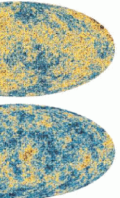
These very obvious differences in the lowest multipoles in some of the realizations are also apparent in the all-sky simulated maps. Figure 11 illustrates this point by showing one of the low quadrupole $\Lambda$CDM realizations and a $\Lambda$CDM realization with the average value of the quadrupole.

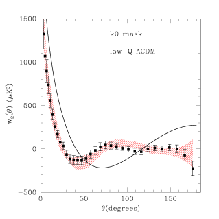
In Figure 12 we show the comparison of $w_{2}(\theta)$ with the low-Q model which is apparently in much better agreement with WMAP.

Figure 10: The 2-point angular correlation $w_{2}$ in the WMAP V-band data (points with jackknife error bars) compared to 10 of the $\Lambda$CDM simulations (continuous lines) which happens to have a low quadrupole and one (dashed line) with a high quadrupole. These are all taken out of the 100 realisations, whose dispersion is shown as the shaded region in Fig.9.

Figure 11: Two of the $\Lambda$CDM simulations, with average (top) and low (bottom) quadrupole.

Figure 12: The 2-point angular correlation $w_{2}$ in the WMAP V-band data (points with jackknife error bars) compared to the low-Q simulations ($\Lambda$CDM model with zero quadrupole, $c_{2}=0$, and 1/2 the octopole $c_{3}/2$). The continuous line shows the $\Lambda$CDM model predictions.

3.3 Covariance Matrix

To quantify these differences more accurately we need to calculate the covariance matrices of the models. We can also estimate the covariance matrix of the data using the jackknife method, Eq. [12]. Figure 13 shows the normalised covariance matrix estimation, which is more similar to the low-Q model than to the $\Lambda$CDM model shown in Fig. 5. Fig. 4 compares the diagonal errors with N=8 and N=32 jackknifes subsamples (continuous lines) with the errors in the low-q and $\Lambda$CDM models.

Figure 13: Normalised covariance matrix from WMAP jackknife samples, to be compared to Fig. 5.

3.4 $\chi^{2}$ tests of the WMAP data

Table 2: Likelihood of WMAP data in different models. First column shows the model we are comparing to, e.g.  $\Lambda$CDM denotes that we are comparing to the mean $w_{2}(\theta)$  of the $\Lambda$CDM simulations. The second column indicates the model from which we take the covariance matrix. The fourth column indicates how many singular values we use in calculating the $\chi^{2}$ and the fifth column is the probability of the fit.

Model	Errors	$\chi^{2}$	Modes	P
$\Lambda$CDM	WMAP	200	7	0
$\Lambda$CDM	$\Lambda$CDM	3.5	5	0.62
low-Q	WMAP	9.6	7	0.21
low-Q	low-Q (true)	4.7	5	0.45
low-Q	low-Q (jackknife)	4.1	6	0.66

Table 3: Likelihood of WMAP data with a galaxy cut in different models

Model	Errors	$\chi^{2}$	Modes	P
$\Lambda$CDM 30	WMAP 30	191	7	0
$\Lambda$CDM 30	$\Lambda$CDM 30	5.7	6	0.46
low-Q 30	WMAP 30	14	7	0.06
low-Q 30	low-Q 30	5.2	7	0.64

Using the method described in the previous section, we compare the WMAP $w_{2}(\theta)$ to different models in Table 2. The second row shows how considering the WMAP data as a realization of the $\Lambda$CDM model gives a very good fit (62% C.L.). However, considering the WMAP jackknife errors (i.e. first row in Table 2) leads to a vanishing probability for the $\Lambda$CDM model, as was already hinted at in Fig.9.

On the other hand, the WMAP data provides a resonable fit to the low-Q models, even if we use the WMAP errors, as can be seen from the third, fourth and fifth row of Table 3. The WMAP data clearly has a low quadrupole compared to $\Lambda$CDM as was already suggested by Figure 13.

Considering only the WMAP data at $|b|>30$ deg, and comparing the resulting $w_{2}(\theta)$ to the models, give similar results as can be seen in Table 3. This is in qualitative agreement with that found by COBE (Kogut et al. 1996).

The above results are obtained with a relatively small number of simulations (40 for $\Lambda$CDM and 20 for low-Q model) and also a small number of jackknife subsamples (16). Thus, although these estimates probably give the right order of magnitude for the calculation we can not expect them to be very accurate. We next quantify what are the errors involved by repeating the $\Lambda$CDM analysis with an increasing number of simulations, from $N=100$ to $N=2000$, to calculate the covariance matrix. We can also check with these additional simulations if the $\chi^{2}$ distribution gives an accurate representation of the probabilities. This is illustrated in Fig.14, which shows the histogram of $\chi^{2}$ values obtained for each $\Lambda$CDM realization using a direct inversion of the covariance matrix (no SVD), estimated from $N=1000$ $\Lambda$CDM realizations. The histogram matches well the probabilities given by the $\chi^{2}$ distribution. Moreover we find that, other than Poisson errors, the values are quite insensitive to the total number $N$ of simulations used. The probability of finding a $\Lambda$CDM simulation with a $\chi^{2}$ value larger than WMAP seems to converge to $32\%$. This number compares well to the crude $62\%$ estimate we found in Table 2 using SVD over 40 simulations. If we used 20 or 100 simulations with SVD we find intermediate results. We have also estimated the $\chi^{2}$ values for $N=2000$ $\Lambda$CDM simulations using the WMAP jacknife covariance matrix. We find that none of the $N=2000$ $\Lambda$CDM simulations have a $\chi^{2}$ smaller than WMAP (the smaller value in the 2000 simulations is $\chi^{2}=62$ for 36 bins in $w_{2}(\theta)$ ). Thus the probability for $\Lambda$CDM given the WMAP errors is $P<0.05$%, in good agreement with first entry in Table 2.

Figure 14: Number of $\Lambda$CDM simulations with given values of $\chi^{2}$ in Eq.13 using the covariance matrix from the same $\Lambda$CDM simulations. The same test for WMAP gives: $\chi^{2}\simeq 39$ (shown by the arrow), which is below $32\%$ of the simulations.

3.5 Recovered $C_{l}$ from $w_{2}(\theta)$

Using the previously discussed method (see §2.11) of calculating the $\chi^{2}$ with the SVD, we can recover the $C_{l}$s from the data by requiring that $\chi^{2}$ has a minimum. Fitting three multipoles ($C_{2},\ C_{3}$ and $C_{4}$) of a $\Lambda$CDM model to the WMAP data and using the $\Lambda$CDM errors yields

$$\mbox{$$}C_{2}=-7\ C_{3}=190\ C_{4}=226.$$ (16)

With the jacknife WMAP errors we get

$$\mbox{$$}C_{2}=123\ C_{3}=217\ C_{4}=212.$$ (17)

Comparing with Eq. 4, we see that the best fit value has a negligible quadrupole and an octopole that is roughly half the value of the $\Lambda$CDM model. Even the $C_{4}$ is somewhat lower than the $\Lambda$CDM value. The low-Q model is hence a better approximation to the $w_{2}(\theta)$ measured from the WMAP data.

Figure 15: Confidence plot of $(C_{2},C_{3})$ (upper panel) and $(C_{2},C_{4})$ (lower panel) recovered from the $\Lambda$CDM model with WMAP (inner contours) and $\Lambda$CDM (outer contours) errors. The contours, in both cases, are at the $0.1,\ 0.68$ and $0.98$ confidence levels. The filled square shows the location of the theoretical $\Lambda$CDM values in both cases.

The confidence contours of the $C_{l}$s are plotted in Fig. 15 for the WMAP errors for the two sets of pairs $(C_{2},C_{3})$ and $(C_{2},C_{4})$. The figure fully confirms our expectations: the WMAP data is in good agreement with $\Lambda$CDM when WMAP data is considered a realization of the $\Lambda$CDM model (i.e. using $\Lambda$CDM errors). The WMAP data is not in agreement with $\Lambda$CDM however when using WMAP errors.

From the confidence plots we can recover the $68\%$ C. L. (or $\sim 1$-sigma) limits for the $C_{l}$s by considering the projections of the contours on the axes. When no model is assumed, i.e. we use WMAP errors, we find (in $\mu K^{2}$):

$$\mbox{$$}C_{2} = 123\pm 233$$

$$C_{3} = 217\pm 241$$

$$C_{4} = 212\pm 162,$$ (18)

which are shown as closed triangles in Fig.1. With a $\Lambda$CDM covariance matrix the errors are much larger (in $\mu K^{2}$),

$$\mbox{$$}C_{2} = -7\pm 1568$$

$$C_{3} = 190\pm 799$$

$$C_{4} = 226\pm 339,$$ (19)

Compared to Eq.2.2, our errors are about a factor of two larger.

Figure 16: Higher-order 2-pt moments in WMAP V-band (continuous line) and WMAP foreground clean map (long-dashed line) as compared with the dispersion in the corresponding measurements in the low-Q $\Lambda$CDM simulations (shaded regions). The short-dashed line in the left-hand panel shows $w_{12}$ from the full combined clean map, ie without the Galactic cut at $|b|<20$.

3.6 Higher-order moments

We also present the higher-order moments of the 2-point correlations in WMAP. This provides a consistency test for the Gaussian hypothesis, which is implied in the comparison with simulations.

The higher-order moments of the 2-point function can be defined as:

$$\mbox{$$}k_{pq}(\theta)\equiv\langle\Delta T^{p}({\bf\theta_{1}})\Delta T^{q}({\bf\theta_{2}})\rangle$$ (20)

where $p=q=1$ corresponds to the 2-point function in Eq.[1], i.e. $k_{11}(\theta)=w_{2}(\theta)$ and $p=0$ gives the 1-point moments, e.g. $k_{02}=k_{11}(0)$ is the variance and $k_{03}=k_{12}(0)$ is the skewness. It is then useful to define 2-point cumulants as connected moments, subtracting the lower-order contributions (e.g. see Gaztañaga, Fosalba & Croft 2002) :

$$\mbox{$$}w_{11}(\theta) \equiv w_{2}(\theta)\equiv k_{11}(\theta)$$ (21)

$$w_{12}(\theta) \equiv k_{12}(\theta)$$ (22)

$$w_{13}(\theta) \equiv k_{13}(\theta)-3k_{11}(0)~{}k_{11}(\theta)$$ (23)

$$w_{14}(\theta) \equiv k_{14}(\theta)-6k_{11}(0)~{}k_{12}(\theta)-4k_{12}(0)~{}k_{11}(\theta)$$ (24)

For a Gaussian field we expect $w_{pq}(\theta)=0$.

It is straightforward to estimate these higher-order moments in the same way in which we have calculated the 2-point function:

$$\mbox{$$}k_{pq}(\theta)={\sum_{i,j}\Delta_{i}^{p}\Delta_{j}^{q}~{}w_{i}^{p}~{}w_{j}^{q}\over{\sum_{i,j}w_{i}^{p}~{}w_{j}^{q}}}.$$ (25)

Here, as in calculating the 2-point function, uniform weights, $w_{i}=1$, are used. We have estimated the higher order moments as well as the covariance matrix both from WMAP and simulated data.

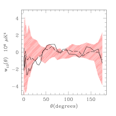
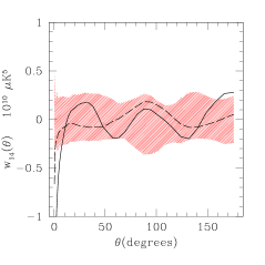
Figure 16 shows $w_{12}$, $w_{13}$ and $w_{14}$ for the WMAP V-band data and the combined foreground clean map in Tegmark et al. (2003) with a Galactic cut excluding $|b|<20$ (long dashed line). Also shown are the 68% CL in the dispersion from the low-Q $\Lambda$CDM simulations. Both WMAP and the combined map with $|b|>20$ agree well with the Gaussian hypothesis $w_{pq}=0$ at high significance.

For the 3rd order moment, $w_{12}$, we also show the combined clean map without the Galactic cut (short-dashed line). This result is incompatible with the Gaussian low-Q $\Lambda$CDM simulations (and covariance matrix) on small angular scales, $\theta<20$ deg. This is in qualitative agreement to what Chiang et al. (2003) have recently found using phase correlators over the very same map. Nevertheless, we note how this apparent discrepancy goes away when we exclude the $|b|<20$ Galactic region. Thus, this non-Gaussian feature seems to be related to residual Galaxy contamination, which is visually apparent in the image of the combined clean map (e.g. see Fig. 1 in Tegmark et al. 2003).

Our best constraints on non-Gaussian features come from the 4th-order statistic, $w_{13}$, because in this case the pixel noise at two different points would tend to cancel out, as in the 2nd-order moment $w_{2}$. This is not the case for the 3rd and 5th-order moments, $w_{12}$ or $w_{13}$, where pixel noise is added in quadrature. One needs to consider multi-point correlations to reduce the noise contribution and get better constraints on non-Gaussian models, which is beyond the scope of this paper (see Hinshaw et al. 1995, Komatsu et al. 2003). The point here is that the higher-order 2-point anisotropies in WMAP are perfectly compatible with the Gaussian hypothesis, given the pixel noise. We find similar results up to 8th-order moments.

4 Conclusions

In this paper we have studied the lowest-order multipoles in the CMB from recent WMAP data. This work is motivated by the fact that the low order multipoles, and especially the quadrupole as measured in harmonic space, show less power than that expected in the standard $\Lambda$CDM model (e.g. see Bennett et al. 2003; Spergel et al. 2003; Peiris et al. 2003). Instead of looking at the power spectrum, we study the WMAP data by using the two-point angular correlation function, $w_{2}(\theta)$ , as a tool to estimate the multipoles. The main advantage is that $w_{2}(\theta)$ is very sensitive to the low order multipoles The main disadvantage is that different bins of $w_{2}(\theta)$ are highly correlated so a covariance analysis is required.

We have simulated a set of V-band maps with different random phases using the best-fit WMAP power spectra and pixel errors, and calculate the 2-point function for each model. Using this set of simulations we calculate the mean value and variance at each bin as well as the covariance matrix. The errors and the covariance matrix of the WMAP data is calculated by using the jacknife method. A $\Lambda$CDM model with a zero quadrupole and a low octopole is also simulated and used to test the reliability of the jacknife errors.

Using a $\chi^{2}$ test with a covariance matrix we calculate the significance of the WMAP data in different models. It is found that indeed, the WMAP data with the WMAP errors does not fit the $\Lambda$CDM model and is strongly disfavoured. Instead, the WMAP data fits well the low-Q model with a vanishing quadrupole. However, taking a different point of view and considering the WMAP data as a sample realization of the simulated $\Lambda$CDM maps, we find that the WMAP results are fully consistent with the $\Lambda$CDM model. From this viewpoint, our sky just happens to have a low quadrupole and is just as likely to have a large quadrupole as demonstrated by the different realizations in Figure 11.

Our results are in apparent contradiction with the harmonic space analysis presented by Spergel et al. (2003), which gives WMAP a probability as low as $0.15\%$ of being a realization of the $\Lambda$CDM model. In contrast we estimate this probability to be $32\%$ comparing $w_{2}(\theta)$ in WMAP to $w_{2}(\theta)$ in 1000 $\Lambda$CDM realizations (see Fig.14). Our probability is closer, but still larger than the $5\%$ value obtained from harmonic analysis by Tegmark etal (2003) Why are all these estimates so different? To answer this question we conduct a further test by repeating our calculation using a different galactic mask. We use a sharp cut in Galactic latitude $|b|$ of about $\pm 20$ degrees, excluding the same number of pixels as the kp0 mask. We then recalculate the covariance matrix and its inversion with this new Galactic cut over the same 1000 $\Lambda$CDM realizations. We repeat the $\chi^{2}$ analysis (in Fig.14) for WMAP and the 1000 simulations with this new covariance matrix. We find that only $1\%$ of the simulations with this Galactic cut have a $\chi^{2}$ larger than the one measured for WMAP. Thus the final probability depends strongly on the shape of the mask, and therefore on how the mask is accounted for in the comparison between the models and observations. This is not surprising because the large scale modes that determine the shape of $w_{2}(\theta)$ (eg Fig.2) extend over angular regions that are comparable to the mask. To recover the low order multipoles from masked data using harmonic decomposition, one needs to invert the convolution with the harmonic image of the mask. This is a non-linear transformation that is likely to introduce biases in the recovered low multipoles. We speculate that the origin of the above discrepancies with the harmonic analysis could depend on how the mask is taken into account on the different estimators. Because the $w_{2}(\theta)$ estimator is independant of the mask we believe that our $\simeq 30\%$ probability value is reliable.

One can also recover the values of the low multipoles from the $w_{2}(\theta)$ WMAP estimations. The validity of the method is demonstrated by recovering known $C_{l}$s from a set of simulated data. Again, we find that the best fit model has a low quadrupole as well as a small octopole. Confidence levels in the $C_{l}$ plane point to a similar conclusion: the WMAP data fits the $\Lambda$CDM model, but only with $\Lambda$CDM priors. We can also reach a similar conclusion by asking how many of the first 100 $\Lambda$CDM simulations show a 2-point function that ”looks” closer to the WMAP data than to $\Lambda$CDM $w_{2}$ (e.g. see Figure10). There is a clear distinction of such cases, which is even apparent by a direct inspection of the pixel-map images (see Figure 11). We find at least 15 similar examples of low quadrupole amongst the first 100 simulations, confirming our more quantitative analysis above.

We have also considered the presence of possible non-Gaussianities in the WMAP data by calculating higher-order moments of the 2-point correlation. We find that both the WMAP and combined foreground clean map of Tegmark et al. (2003) at $|b|>20$ are in excellent agreement with the Gaussian hypothesis. It is also shown how the full-sky foreground clean map (i.e. including $|b|<20$ ) shows a non-Gaussian feature at angular scales $\theta<20$ degrees, indicating a possible residual galaxy contamination in the map.

In summary, the low value of the WMAP quadrupole is confirmed here by looking at the two-point angular correlation function, $w_{2}(\theta)$ , which is shown to be a well-suited method for the study of low multipoles in the CMB data. This does not necessarily indicate a need for new physics or non-standard cosmology, since we also show the WMAP $w_{2}(\theta)$ fits well a standard $\Lambda$CDM cosmology if one considers our universe as a realization of the set of possible $\Lambda$CDM outcomes. We stress nevertheless, that by considering the errors from the WMAP data alone, i.e. with the jacknife errors, $w_{2}(\theta)$ in WMAP is strongly inconsistent with the mean $\Lambda$CDM model and, under such an assumption, new ideas to explain the discrepancy could well be in order. Finally, we have demonstrated that our conclusions are robust when we exclude data with Galactic latitudes $|b|<30$, which indicates that the information (or lack of information) in the Galactic plane is not responsible for the missing large scale power.

References

- (1) Bennett C.L. et al. , 2003, preprint (astro-ph/0302207).
- (2) Bond J.R. & Efstathiou G., 1987, MNRAS, 226, 655.
- (3) Chiang, L-Y., Naselsky, P.D., Verkhodanov, O.V., Way, M.J. astro-ph/0303643
- Contaldi et al. (2003) Contaldi C.R., Peloso M., Kofman L., Linde A., 2003, preprint (astro-ph/0303636).
- (5) Gaztañaga, E, Fosalba, P., Croft, R.A.C. MNRAS, 331, 13.
- (6) Efstathiou G., 2003a, preprint (astro-ph/0303127).
- (7) Efstathiou G., 2003b, preprint (astro-ph/0306431).
- (8) Górski, K. M., Hivon, E., & Wandelt, B. D., 1999, in Proceedings of the MPA/ESO Cosmology Conference ”Evolution of Large-Scale Structure”, eds. A.J. Banday, R.S. Sheth and L. Da Costa, PrintPartners Ipskamp, NL, pp. 37-42 (also astro-ph/9812350)
- (9) Hinshaw G., Banday A.J., Bennett C.L., Gorski K.M., Kogut A., 1995, ApJ, 446, L67.
- (10) Hinshaw G., Banday A.J., Bennett C.L., Gorski K.M., Kogut A., Smoot G.F., Wright E.L., 1996, ApJ, 464, L17.
- (11) Hinshaw G., Banday A.J., Bennett C.L., Gorski K.M., Kogut A., Lineweaver, C,H., Smoot G.F., Wright E.L., 1996, ApJ, 464, L25.
- (12) Kogut A., Banday A.J., Bennett C.L., Gorski K.M., Hinshaw G., Smoot G.F., Wright E.L., 1996, ApJ, 464, L5.
- (13) Komatsu, E. et al. 2003, preprint (astro-ph/0302223).
- (14) Landy, S.D. & Szalay, A.S., 1993, ApJ, 412, 64
- (15) Peiris H.V. et al. , 2003, preprint (astro-ph/0302225).
- (16) Seljak, U., Zaldarriaga, M., 1996, ApJ, 469, 437
- (17) Spergel D.N. et al. , 2003, preprint (astro-ph/0302209).
- (18) Szapudi, I, Prunet, S., Pogosyan, D., Szalay, A., Bond, R., 2001, ApJ 548, L11
- (19) Tegmark M., de Oliveira-Costa A., Hamilton A., 2003, preprint (astro-ph/0302496).