Numerical Methods in Gravitational Lensing

Abstract

Most problems in gravitational lensing require numerical solutions. The most frequent types of problems are (1) finding multiple images of a single source and classifying the images according to their properties like magnification or distortion; (2) propagating light rays through large cosmological simulations; and (3) reconstructing mass distributions from their tidal field. This lecture describes methods for solving such problems. Emphasis is put on using adaptive-grid methods for finding images, issues of spatial resolution and reliability of statistics for weak lensing by large-scale structures, and methodical questions related to shear-inversion techniques.

1 Introduction

Only for very special lens models can numerical methods be avoided in gravitational lensing studies. There are three essential reasons for that. One is the non-linearity of gravitational lensing, i.e. the fact that image and source positions are related to one another in a non-linear fashion. This gives rise to the well-known phenomena of mutiple imaging, strong image distortions, and so forth. The second reason is that lenses exist which are themselves best described by numerical models. Galaxy clusters are one example, lensing by large-scale structures is another. Although it is true that many aspects of gravitational lensing by large-scale structures can be derived analytically, detailed simulations require numerical techniques. The third reason is that the interpretation of gravitational lensing effects or events often require the application of sophisticated algorithms to ever growing amounts of data. One example is the reconstruction of the projected mass density distribution of a galaxy cluster from the observed image distortions due to gravitational shear.

Needless to say, there are many more aspects of numerical methods related to gravitational lensing than I can cover in this review. An outstanding example are the highly elaborate methods that have been developed over recent years for determining image shapes of faint background galaxies on CCD frames, and for extracting the gravitational shear signal from them. This is a whole branch of data analysis on its own. Here, I can only deal with numerical methods for relating mass distributions to their gravitational lensing effects.

Consequently, the outline of this lecture is as follows: First, I shall discuss methods for studying individual lenses, i.e. their imaging properties, their critical curves and caustics. In particular, the use of adaptive grids and techniques for searching and characterising images will be discussed. Second, I shall describe how extended lenses can be treated numerically using the multiple-lens plane theory. This will lead to the basic equations for tracing light rays through (simulated) cosmological volumes. A large fraction of the discussion will be devoted to issues of resolution and noise, and to spurious effects in simulated lensing statistics. Finally, third, I shall describe inversion techniques, i.e. methods for reconstructing the projected mass distribution of lenses whose distortion has been measured. The classic Kaiser-Squires method will be described, and also maximum-likelihood techniques and maximum-entropy methods.

General lensing theory and the theory of weak lensing are covered by Koenraad Kuijken’s and Peter Schneider’s lectures in this volume. Basic references on lensing include the textbook by Schneider et al. (1992) and the lecture by Narayan & Bartelmann (1999), reviews of weak lensing are Mellier (1999) and Bartelmann & Schneider (2001).

2 Individual Lenses

2.1 Assumptions

A brief reminder of the basic assumptions underlying the theory of individual lenses may be in order. There are three main assumptions. First, the Newtonian gravitational potential of the lens be small, $|\Phi|\ll c^{2}$. Second, velocities in the gravitational lens system, both of constituents within the lenses and of the lenses with respect to the rest frame of the microwave background, be small $v\ll c$. Third, the extent of the lenses along the line-of-sight be small compared to the other distances in the system, which are usually cosmological and thus comparable to the Hubble radius, $c/H_{0}=3\,h^{-1}\,\mathrm{Gpc}$, with $H_{0}$ being the Hubble constant and $h=H_{0}/100\,\mathrm{km\,s^{-1}\,Mpc^{-1}}$.

It is worth noting how well these assumptions are satisfied in ordinary lensing situations. Consider a galaxy cluster with mass $M=10^{15}\,h^{-1}M_{\odot}$. Assuming spherical symmetry, the Newtonian potential at a distance $R=1\,h^{-1}\,\mathrm{Mpc}$ from its centre is

$$|\Phi|\approx\frac{G\,M}{R}\approx(2\times 10^{3}\,\mathrm{km\,s^{-1}})^{2}\;,$$ (1)

evidently much smaller than the speed of light squared. A typical length scale for the radius of a galaxy cluster is $1-1.5\,h^{-1}\,\mathrm{Mpc}$, which is several hundred times smaller than typical distances in a cluster-lensing system. Finally, peculiar velocities of galaxy clusters with respect to the Hubble flow are of order several hundred $\mathrm{km\,s^{-1}}$, and typical velocities of galaxies within galaxy clusters reach of order $10^{3}\,\mathrm{km\,s^{-1}}$, but both velocities are way below the speed of light. The above assumptions hold even better for lensing by galaxies, of course.

We can thus safely assume the above conditions to be satisfied. It is then possible to project the lensing mass distribution onto a plane perpendicular to the line-of-sight, the lens plane, and describe it by its surface mass density $\Sigma$. Sources are assumed to be located on a corresponding plane, the source plane. A typical lens system is sketched in Fig. 1.

Figure 1: Schematic view of a gravitational lens system. The lens is projected onto the lens plane perpendicular to the line-of-sight, sources are located on the parallel source plane. There are three distances required to describe the geometry of the system, i.e. the distances $D_{\mathrm{d,s,ds}}$ between the observer and the lens, the observer and the source, and between the lens and the source, respectively. Due to space-time curvature, these distances are generally not additive.

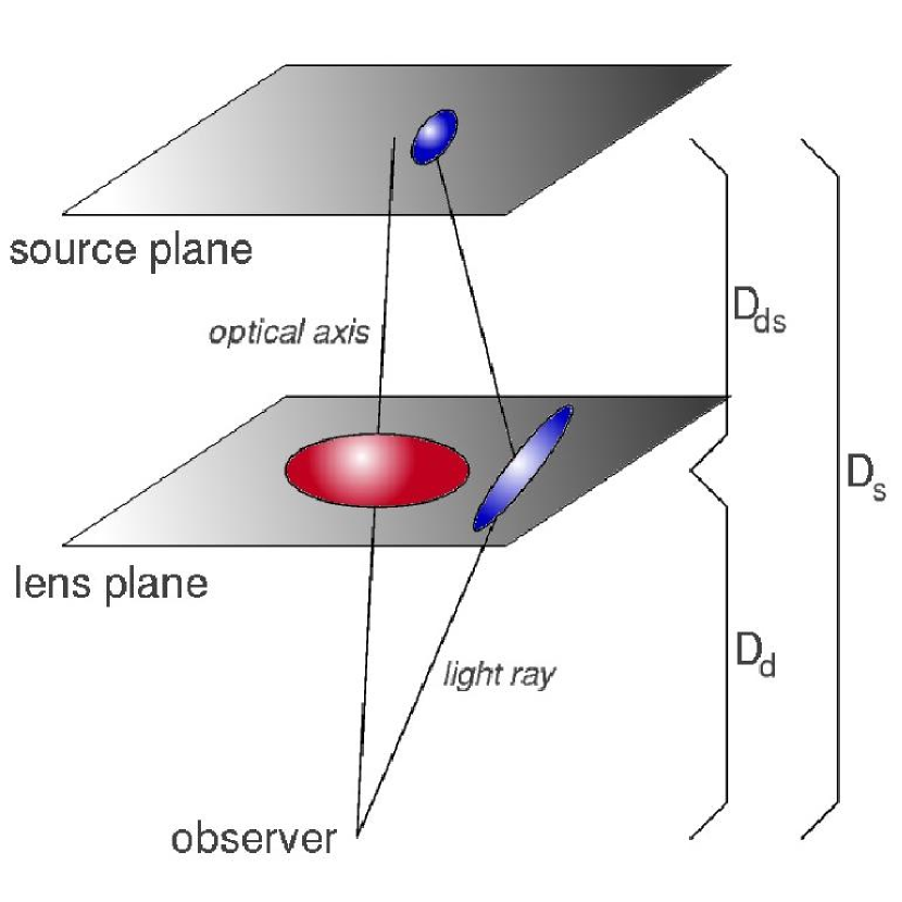
The three distances $D_{\mathrm{d,s,ds}}$ shown in Fig. 1 and explained in its caption are generally not additive because of space-time curvature, thus $D_{\mathrm{s}}\neq D_{\mathrm{d}}+D_{\mathrm{ds}}$ in contrast to flat space-time.

2.2 Coordinates and Notation

Let us now introduce physical coordinates $\vec{\xi}$ and $\vec{\eta}$ on the lens and source planes, respectively. Alternatively, it is often convenient to introduce angular coordinates $\vec{\theta}$ and $\vec{\beta}$, which are obviously related to $\vec{\xi}$ and $\vec{\eta}$ through

$$\vec{\xi}=D_{\mathrm{d}}\,\vec{\theta}\;,\quad\vec{\eta}=D_{\mathrm{s}}\,\vec{\beta}\;.$$ (2)

Dimensional coordinates are of course not suitable for numerical calculations, which can only handle numbers. We thus have to introduce a length scale $\xi_{0}$, or alternatively an angular scale $\theta_{0}$, in the lens plane. This length scale is so far arbitrary. It implies a length or angular scale

$$\eta_{0}=\frac{D_{\mathrm{s}}}{D_{\mathrm{d}}}\,\xi_{0}\;,\quad\mbox{or}\quad\beta_{0}=\frac{\eta_{0}}{D_{\mathrm{s}}}=\frac{\xi_{0}}{D_{\mathrm{d}}}=\theta_{0}$$ (3)

in the source plane. Dimension-less coordinates are then defined by

$$\vec{x}=\frac{\vec{\xi}}{\xi_{0}}=\frac{\vec{\theta}}{\theta_{0}}\;,\quad\mbox{or}\quad\vec{y}=\frac{\vec{\eta}}{\eta_{0}}=\frac{\vec{\beta}}{\theta_{0}}$$ (4)

in the lens and source planes, respectively. The numerical code will have to deal with the dimension-less vectors $\vec{x}$ and $\vec{y}$. It helps numerical accuracy greatly if these numbers are of order unity. Thus, the first challenge in setting up a lensing simulation is to choose an appropriate length- or angular scale $\xi_{0}$ or $\theta_{0}$, which should both be adapted to the physical problem at hand, and to the requirement that numerical codes work most accurately if the numbers they are dealing with are neither too large nor too small, compared to machine accuracy. Choosing unappropriate length scales can, for instance, render image searches unsuccessful.

2.3 The Lensing Potential

It will be convenient for the following discussion to introduce the lensing potential $\psi$ as the basic physical quantity for lensing studies. It is the scaled, projected Newtonian gravitational potential of the lens,

$$\psi(\vec{x})=\frac{2}{c^{2}}\,\frac{D_{\mathrm{d}}D_{\mathrm{ds}}}{\xi_{0}^{2}\,D_{\mathrm{s}}}\,\int\,\Phi(\xi_{0}\vec{x},l)\,\mathrm{d}l\;.$$ (5)

The so-called reduced (i.e. appropriately scaled) deflection angle is the gradient of the potential,

$$\vec{\alpha}(\vec{x})=\nabla_{\vec{x}}\psi(\vec{x})\;,$$ (6)

and the lensing convergence (i.e. the appropriately scaled surface-mass density) is

$$\kappa(\vec{x})=\frac{1}{2}\,\nabla_{\vec{x}}^{2}\psi(\vec{x})=\frac{1}{2}\,\nabla_{\vec{x}}\cdot\vec{\alpha}(\vec{x})\;.$$ (7)

Finally, the gravitational tidal field is described by the two-component shear,

$$\gamma_{1}(\vec{x})=\frac{1}{2}\left(\psi_{,11}-\psi_{,22}\right)=\frac{1}{2}\left(\alpha_{1,1}-\alpha_{2,2}\right)\;,\quad\gamma_{2}(\vec{x})=\psi_{,12}=\alpha_{1,2}\;,$$ (8)

where the convention was used that $f_{i,j}$ is the derivative of the $i$-th component of $\vec{f}$ with respect to the coordinate $x_{j}$. It is important to note that the fact that all lensing quantities can be derived from the scalar lensing potential establishes relations between all of them. This will be exploited several times later.

Note that the lensing quantities must be rescaled in case the coordinate scale $\xi_{0}$ is changed. Suppose $\xi^{\prime}_{0}$ is introduced instead of $\xi_{0}$. Since the physical surface-mass density of the lens must remain the same at any given physical location, the reduced deflection angle must transform as

$$\vec{\alpha}(\vec{x}^{\prime})=\frac{\xi_{0}^{\prime}}{\xi_{0}}\,\vec{\alpha}(\vec{x})\;,$$ (9)

and convergence and shear transform as

$$\left[\kappa(\vec{x}^{\prime})\,,\,\gamma_{i}(\vec{x}^{\prime})\right]=\left(\frac{\xi_{0}^{\prime}}{\xi_{0}}\right)^{2}\,\left[\kappa(\vec{x})\,,\,\gamma_{i}(\vec{x})\right]\;.$$ (10)

2.4 Imaging

Suppose now we were given some description of the lensing potential $\psi(\vec{x})$, or of the deflection angle $\vec{\alpha}(\vec{x})$. This description could be an analytical formula, or it could be in form of an array, i.e. a set of numbers given at grid points $(x_{i},x_{j})$. We wish to know how the given lens images its background.

We introduce a coordinate grid $\vec{x}_{ij}$ on the lens plane subject to the condition that it be sufficiently well resolved. This means that the smallest features in the lens must be covered by at least a few grid points. Since we are given the deflection angle as a function of position, we can compute a deflection-angle grid, $\vec{\alpha}_{ij}=\vec{\alpha}(\vec{x}_{ij})$. The mapped grid on the source plane is then simply $\vec{y}_{ij}=\vec{x}_{ij}-\vec{\alpha}_{ij}$. This mapped grid will appear as a distorted image of the regular grid in the lens plane, as the example in the left panel of Fig. 2 shows.

Figure 2: Left panel: A regular grid in the lens plane (blue dots) is mapped onto the source plane (red dots) using a numerical description of a deflection-angle field. Distortions are clearly visible. Right panel: For each point in the lens plane, those points of a regular grid in the source plane (blue) are searched which surround its mapped point in the source plane (red).

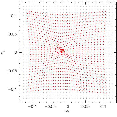
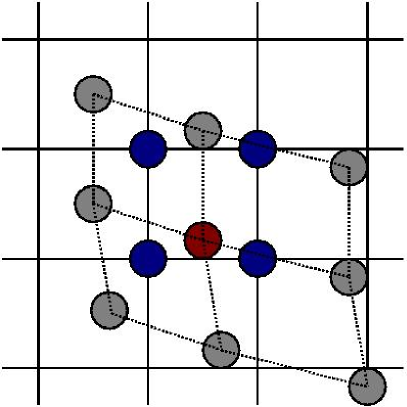
The mapping process must now be reversed in order to obtain an image created by the lens. For doing so, the source plane is first covered with a regular grid, $\vec{y}_{ij}^{\prime}$. Next, we loop over all grid points $\vec{x}_{ij}$ in the lens plane and find its mapped source point $\vec{y}_{ij}$ in the source plane, and search for the nearest neightbours $\vec{y}_{kl}^{\prime}$ surrounding $\vec{y}_{ij}$ in the source plane. This is illustrated in the right panel of Fig. 2. The surface brightness of the source, known at the positions $\vec{y}_{kl}^{\prime}$, can then be interpolated to $\vec{y}_{ij}$ and the result assigned to the image point $\vec{x}_{ij}$. That way, the surface brightness at all points in the lens plane can be determined, and thus the lensed image be constructed. Fig. 3 shows an example.

Figure 3: Left panel: A simulated CMB temperature fluctuation field of $10^{\prime}\times 10^{\prime}$ size. Right panel: The same field, lensed by a galaxy cluster, which imprints a characteristic pattern on the temperature fluctuations.

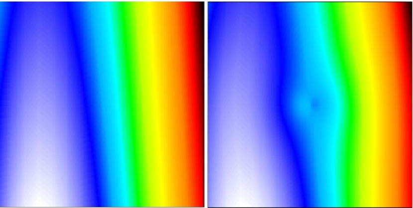
The left panel of the figure shows a simulated CMB temperature fluctuation field of $10^{\prime}\times 10^{\prime}$ angular size. The temperature increases from white to red. In essence, the temperature fluctuation corresponds to a fairly smooth gradient across the field. The right panel shows the gravitational lensing signature imprinted on the CMB at such angular scales by a galaxy cluster. The temperature visible at an angular position $\vec{\theta}$ on the sky, $T^{\prime}(\vec{\theta})$, is related to the intrinsic temperature $T$ through $T^{\prime}(\vec{\theta})=T[\vec{\theta}-\vec{\alpha}(\vec{\theta})]$. Thus, the light deflection by the cluster causes the visible temperature distribution to be rearranged, yielding a highly specific pattern (Seljak & Zaldarriaga 2000).

2.5 Critical Curves and Caustics

As mentioned in the introduction, the deflection-angle field contains full information on the lensing mass distribution. All other quantities like convergence and shear, but also image magnifications, follow from the deflection angle via differentiation. It is thus a common task to compute numerical derivatives.

Suppose a function $f(\vec{x})$ is tabulated on a grid, so that we are given the values $f_{ij}$ at the grid points $\vec{x}_{ij}$. The derivative of $f(\vec{x})$ at a particular point $\vec{x}_{00}$ in the first coordinate direction is approximated by

$$\left.\frac{\partial f(\vec{x})}{\partial x_{1}}\right|_{\vec{x}_{00}}=\frac{1}{2h}\,\left(f_{10}-f_{-10}\right)+\mathcal{O}(h^{2})\;\,$$ (11)

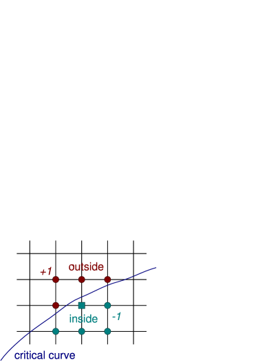
where $h$ is the separation of the grid points in the chosen direction; cf. the left panel of Fig. 4. This centred difference has the advantage compared to the more straightforward one-sided differences $f_{10}-f_{00}$ or $f_{00}-f_{-10}$ of being second-order in the grid separation $h$. There are higher-order differencing schemes using function values at more than two grid points, but the second-order scheme is usually sufficient. No lensing quantity should vary strongly between two adjacent grid points because otherwise the resolution of the grid would be grossly insufficient.

Figure 4: Left panel: Second-order numerical differentiation using centred differences. Right panel: A simple method for finding points in the lens plane next to a critical curve uses sign changes of the Jacobian determinant between the point considered and its four nearest neighbours.

We will typically need derivatives of the deflection angle $\vec{\alpha}$. Since $\vec{\alpha}$ is itself the gradient of a scalar potential, its derivatives must satisfy $\alpha_{1,2}=\psi_{,12}=\psi_{,21}=\alpha_{2,1}$. It is thus usually preferable to check that this relation is satisfied within numerical accuracy, and to use $(\alpha_{1,2}+\alpha_{2,1})/2$ instead of either $\alpha_{1,2}$ or $\alpha_{2,1}$ alone.

Critical curves in the lens plane are defined by the condition that the Jacobian determinant of the lens mapping vanish there, $\det\mathcal{A}(\vec{x})=0$. The elements of the Jacobian matrix are $\mathcal{A}_{ij}=\delta_{ij}-\alpha_{i,j}$, thus the Jacobian determinant is

$$D\equiv\det\mathcal{A}=(1-\alpha_{1,1})(1-\alpha_{2,2})-\alpha_{1,2}^{2}\;.$$ (12)

It can be computed once the (numerical) derivatives of the both deflection-angle components have been determined.

One method of identifying grid points in the lens plane next to the critical curve proceeds as follows. Let $S=\mathrm{sign}(D)$, and consider one particular grid point $\vec{x}_{00}$ in the lens plane. The point is next to the critical curve if, and only if, the sign of the Jacobian determinant changes between it and one or more of its nearest neighbours. Hence, if the condition

$$S_{00}(S_{-10}+S_{10}+S_{0-1}+S_{01})<4$$ (13)

is satisfied, the grid point $\vec{x}_{00}$ is next to a critical curve (cf. the right panel of Fig. 4). Of course, $\vec{x}_{00}$ is not itself on the critical curve, but to the positional accuracy determined by the grid resolution, the position of the critical curve can be constrained that way. Points on the source plane next to the caustic curve are then easily found via the lens equation, $\vec{y}_{\mathrm{C}ij}=\vec{x}_{\mathrm{C}ij}-\vec{\alpha}(\vec{x}_{\mathrm{C}ij})$, where the $\vec{x}_{\mathrm{C}ij}$ are the grid points in the lens plane next to critical curves.

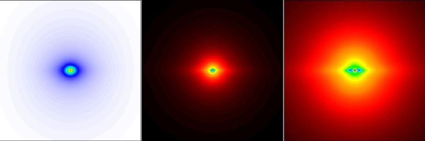
As an example, consider a lens model for a spiral galaxy, consisting of a spherical halo and a flat disk seen almost edge-on (Bartelmann & Loeb 1998). The deflection-angle field of such a lens can be given analytically (cf. Keeton & Kochanek 1998). Convergence and total shear $(\gamma_{1}+\gamma_{2})^{1/2}$ as determined by numerical differentiation are shown together with the modulus of the deflection angle in Fig. 5.

Figure 5: A lens model for an almost edge-on spiral galaxy: shown are the modulus of the deflection angle (left), the convergence (centre), and the absolute value of the shear (right).

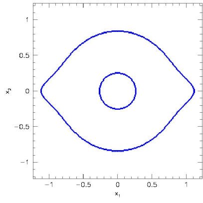
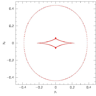
The critical curves and caustics of that lens model as determined with the method described above are shown in Fig. 6.

Figure 6: Critical curves (left) and caustics (right) of the spiral-galaxy lens model illustrated in Fig. 5.

2.6 Adaptive Source Grids

One of the most prominent goals of gravitational lensing studies with individual strong lenses is to determine the imaging statistics of a given lens model, for example the abundance of highly magnified events, the occurrence of multiple imaging with the images satisfying certain conditions, and the like. This is done in principle by distributing many sources across the source plane, imaging them as described before, and determining the image properties. However, such events are rare. If one were to cover the entire source plane with a regular grid of sources, this grid would have to have a very high resolution for rare events to be reliably found. In turn, most of the sources probed would produce images failing the criteria imposed, so by far the largest fraction of the CPU time used would be wasted.

This situation calls for adaptive grids. We know in advance that any strongly lensed image will occur near a critical curve, or any strongly lensed source near a caustic. It is those sources that we need to treat in detail, while those far from caustic curves are usually only required to normalise the statistics properly.

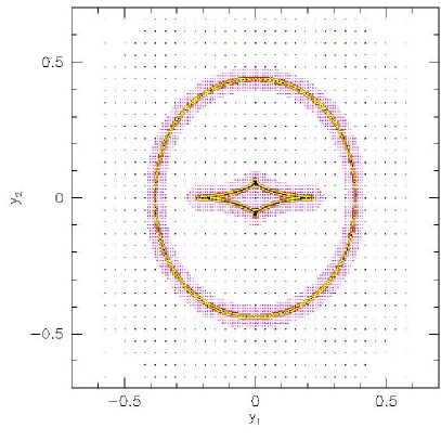
One approach for defining an adaptive grid, and there may be others more suitable for a particular lensing situation, proceeds as follows. Again, we assume that we know the deflection angle of the lens, either because it was provided numerically or because it is described by a known analytic formula. Then, we saw in the preceding subsection how grid points can easily be identified which are close to a critical curve in the lens plane, or a caustic curve in the source plane.

In order to save computational time, the source plane is first covered with a coarse grid. This grid should obviously be fine enough for the caustics to be properly resolved; for instance, it must not be so coarse that the typically two types of caustic curve, the radial and the tangential one, are closer than a few times the grid separation.

Next, those points on that coarse grid are identified and saved which are next to a caustic curve. This can, for instance, be done by masking, i.e. by attaching a logical variable to all grid points and setting it to either true or false depending on whether it is or is not next to a critical curve. One can then cover the source plane with a grid whose resolution is doubled in both dimensions, and keep only those points which are identical with, or surrounded by, points of the coarse grid which were masked in the preceding step. This procedure can be repeated as often as desired, i.e. until the finest grid level reaches the ultimately required resolution. Note that it is not the grids and their masks which need to be saved, but only the coordinates of those grid points which are either part of the coarse initial grid, or whose logical mask values are true. That way, lists of source positions can be constructed which are to be probed later for the images they give rise to.

Naturally, this can only be a basic recipe which needs to be adapted to the situation at hand. For instance, the condition that grid points need to be next to a caustic can be replaced by the condition that the absolute value of the Jacobian determinant be less than a given threshold which can be lowered at each step of grid refinement. Such a criterion would naturally increase the grid resolution near such grid positions where sources are certain to be highly magnified.

Of course, if statistics is the ultimate goal, one has to take into account that sources near caustic curves were positioned such as to have an unfair advantage over sources far from caustics. Since we have chosen to double the grid resolution at each refinement step, each source on a refined grid represents only a quarter of the area on the source plane represented by a source on the next coarser grid. Assigning a statistical weight of unity to the sources on the finest grid, the weight must quadruple for each coarser level. If the grid was refined $N$ times, the weight of sources on the coarsest grid is thus $w_{i}=2^{2N}$. Each source is assigned a statistical weight $w_{i}$ in that way, and counts $w_{i}$ times in the final statistical evaluation.

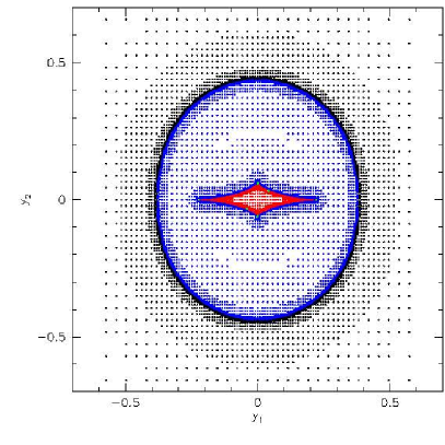
The left panel in Fig. 7 shows the source locations chosen for evaluating image statistics of the spiral lens model illustrated in Fig. 6.

Figure 7: Left panel: source positions placed on a multiply refined grid in the source plane. Caustic points are black. Obviously, the source plane is best sampled near caustics. Right panel: Number of images found for sources placed at the positions shown in the left panel.

2.7 Finding Images

The principle of finding the images of a given source is simple: Given a source at position $\vec{y}_{\mathrm{s}}$, find those grid points $\vec{x}_{ij}$ on the lens plane which are mapped sufficiently close to $\vec{y}_{\mathrm{s}}$, i.e. whose mapped points $\vec{y}_{ij}$ are within a specified distance from $\vec{y}_{\mathrm{s}}$.

The problem with this approach is that a square-shaped or rectangular grid cell from the image plane is mapped onto a distorted figure in the source plane. In most cases, this figure will be a parallelogram, but in rare cases, opposing corners of the original rectangle may even be interchanged on the source plane. How can it then be decided whether a given point in the source plane is inside or outside the mapped grid cell, or in other words, whether the image of the given source falls within that particular grid cell on the lens plane?

The solution is to split each grid cell in the lens plane into two triangles, because a mapped triangle always remains a triangle, which always has a well-defined interiour (cf. Schneider et al. 1992).

Figure 8: Illustration of the technique for finding images described in the text. Grid cells in the lens plane are split into triangles (left panel), which have a well-defined interior after being mapped back onto the source plane (right panel). This would not necessarily be the case for rectangular grid cells. A source is contained by a triangle if all mixed cross products $\vec{d}_{i}\times\vec{d}_{j}$ for the shown vectors $\vec{d}_{i}$ are positive.

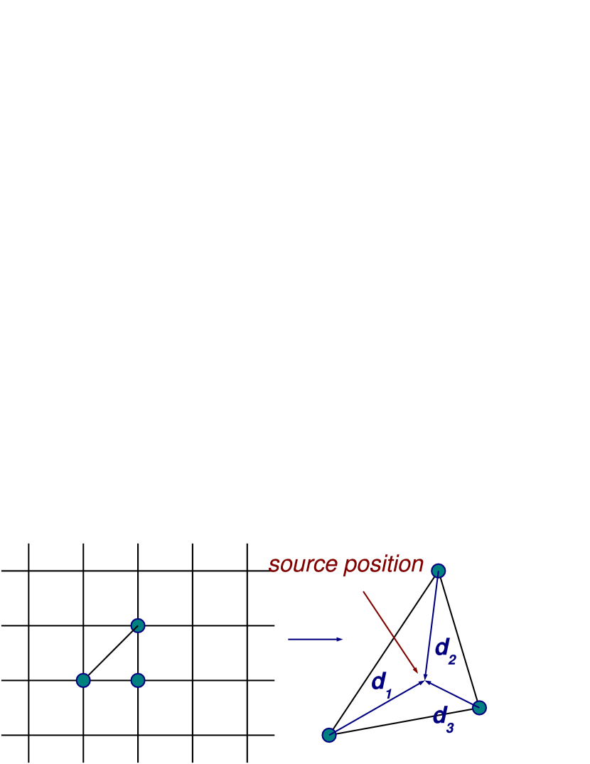
Consider Fig. 8. The three grid points marked on the lens plane in the left panel of the figure are mapped to the distorted triangle shown on the right panel, which contains the source position. Call $\vec{d}_{1,2,3}$ the three vectors from the mapped triangle’s corners towards the source position. It can be shown that the source is inside the mapped triangle if the three vector products

$$\vec{d}_{1}\times\vec{d}_{2}\;,\;\vec{d}_{1}\times\vec{d}_{3}\;,\;\vec{d}_{2}\times\vec{d}_{3}$$ (14)

are all positive, with the vector product in two dimensions being defined as

$$\vec{a}\times\vec{b}\equiv a_{1}b_{2}-a_{2}b_{1}\;.$$ (15)

One straightforward way to verify this condition is to convince one’s self that the source point is inside the triangle if all vectors $\vec{d}_{i}$ point within the angles spanned by the adjacent sides of the triangle, and that this condition translates to Eq. (14) above.

This algorithm for finding images works well as long as the separation between images is larger than the size of the grid cells in the lens plane. Very close images can be contained within the same grid cell, in which case the algorithm would find only one. Of course, this potential problem can be remedied by increasing the grid resolution, but then a very large number of grid cells would have to be checked in vain for containing an image.

Again, a viable solution uses adaptive grids. One can start with a coarse grid on the lens plane. Searching for images on that coarse grid will almost certainly not yield all images of a multiply imaged source, but those missed will be closer than the grid separation to those found. Then, those grid cells containing images can individually be covered with a highly resolved grid, and the image search repeated on those sub-grids. Hence, the first step represents a coarse scan of the lens plane for grid cells containing at least one image, and the second step scans only those regions on the lens plane in detail where images are sure to be found. If needed, further sub-grids can be similarly nested.

Of course, even though this procedure is highly adaptive and efficient, it always has a remaining resolution limit, and images closer than that will not be resolved. It is then important to adapt the resolution of the finest sub-grid to the situation at hand, for instance such that remaining unresolved images would neither be resolved by observations. The right panel in Fig. 7 illustrates the result of an adaptive image search for all sources at the positions shown in the figure’s left panel. Colours denote image numbers: Black means one image, blue three, and red five, while green shows source positions for which an even number of images has been found, in contradiction to the necessarily odd image number produced by non-singular lenses. Such events are rare, but they do occur because of the finite resolution limit of the algorithm applied.

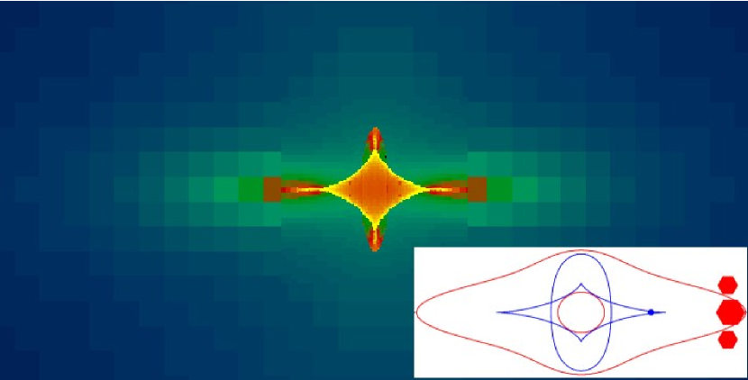
Figure 9 gives an example for possible results of that adaptive technique for finding images. Colour-coded is the total magnification of point sources in the source plane behind the almost edge-on spiral lensing galaxy introduced above. The increasing spatial resolution towards the caustic curves is evident. The panel inserted into the figure shows caustics (blue) and critical curves (red) of the lens, the source position as a blue dot just inside the right-hand “naked” cusp, and the three images as red hexagons whose size logarithmically encodes the image magnification.

Figure 9: The colour encodes the total magnification of a point source lensed by an almost edge-on spiral galaxy; blue means a magnification near unity, yellow means very high magnification. The adaptive resolution of grid cells on the source plane is clearly visible. The size of the grid cells decreases substantially towards regions of high magnification. The inserted panel shows caustics and critical curves of the same lens (blue and red, respectively), a source position close to the right-hand “naked” cusp, and the three images as red hexagons, whose size logarithmically encodes their magnification.

2.8 Asymmetric Lenses

So far, we have used a model for a spiral galaxy as an example for a complex lens whose properties need to be determined numerically. Despite its complexity, the model is still highly symmetric; and what is more, its deflection angle is given as an analytic formula. Sources were so far assumed to be point-like.

Let us now increase the level of complexity and use a numerically simulated galaxy cluster to gravitationally lens extended sources. Again, we assume the deflection angle to be given and postpone the question as to how it can be determined from an $N$-body simulation.

All techniques described above for computing convergence and shear from the deflection angle, for finding critical curves and caustics, for placing sources on an adaptive grid, and for finding images within grid cells split into triangles remain valid unchanged. Figure 10 shows an example.

Figure 10: The colour plot in the left panel shows the modulus of the deflection-angle field in the lens plane of a numerically simulated galaxy cluster. The right panel shows how sources are adaptively placed on the source plane (dots), and how many images these sources have; one (black), three (blue) or five (red). The boundaries between the colours mark the caustic structure.

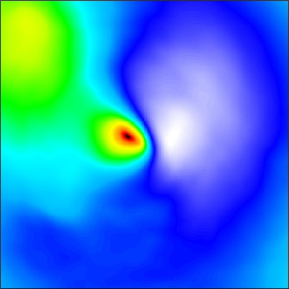
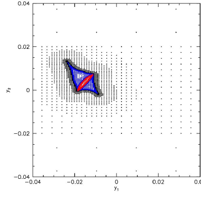
The modulus of the cluster’s deflection angle is shown as the colour plot in the left panel. The right panel shows a section of the source plane with the dots marking source positions, and their colour illustrating the image number. Black, blue and red means one, three, or five images, respectively. The caustic structures can clearly be identified as the boundaries between black and blue and between blue and red, respectively.

2.9 Imaging Extended Sources

Extended sources can be described in a variety of ways. What follows is a simple description for elliptical sources, but alternative source models can easily be constructed along similar lines. We assume that source positions $\vec{y}_{\mathrm{s}}$ have already been found, preferentially on an adaptive grid as described before. Also, we need to be sure that the grid resolution in the source plane is sufficiently high as to resolve the smallest sources to be considered.

Elliptical sources are described by three more parameters, viz. their size, their ellipticity, and their position angle $\phi$. Let us describe the ellipticity by $e=b/a$, with $a$ and $b$ being the semi-major and semi-minor axes of the ellipse, respectively. Finally, we introduce an effective radius $r$ by demanding that a circle of radius $r$ have the same area as the ellipse, hence $r=\sqrt{ab}$. By rotating by an angle $\phi$ an ellipse centred on the coordinate origin whose axes are aligned with the coordinate axes, it can straightforwardly be shown that a grid point $\vec{y}_{ij}$ is enclosed by the ellipse if the condition

$$\cos^{2}\phi\left(\frac{\delta y_{1}^{2}}{e}+e\delta y_{2}^{2}\right) + \sin^{2}\phi\left(\frac{\delta y_{2}^{2}}{e}+e\delta y_{1}^{2}\right)$$ (16)

$$+ 2\delta y_{1}\delta y_{2}\sin\phi\cos\phi\left(\frac{1}{e}-e\right)\leq r^{2}$$

is satisfied, where $\delta\vec{y}\equiv\vec{y}_{ij}-\vec{y}_{\mathrm{s}}$. If the grid point $\vec{x}_{ij}$, whose image in the source plane is $\vec{y}_{ij}$, satisfies Eq. (16), the image point $\vec{x}_{ij}$ is part of the source, and the image can be constructed by assigning the source’s surface brightness at $\vec{y}_{ij}$ to the image point $\vec{x}_{ij}$. By mapping the entire lens plane onto the source plane and checking Eq. (16) for each individual imaged grid point $\vec{y}_{ij}$, all image points belonging to the given source can be identified.

It is often desired for statistical purposes to automatically characterise a large number of images. An example is the determination of cross sections for the formation of large gravitational arcs by a numerically simulated galaxy cluster, for which a large number of sources need to be imaged and the image properties automatically quantified to search for the rare “giant” arcs. Most of the methods described here have been introduced and used extensively e.g. by Bartelmann & Weiss (1994), Bartelmann et al. (1995, 1998), Meneghetti et al. (2000, 2001); see also the contribution by Massimo Meneghetti to this volume.

A source may have multiple images, thus the point sets in the lens plane found by imaging extended sources need not be connected. The first step is therefore to group the image points into images. This can be done with a variant of the classical friends-of-friends algorithm: Pick one arbitrary point out of any given set of image points and search for another image point which is at most $\sqrt{2}h$ grid units away from the first point; $h$ is the grid size in the lens plane. If there is such a point, it is called a “friend” and grouped into the same image as the first point. Now take the “friend” and repeat until no further “friends” can be found and the image is complete. If more image points are left on the lens plane, pick one of those and repeat the process until all image points have been grouped. If the image is large enough, and the grid resolution on the lens plane is high enough for the image to consist of many points, the image magnification is simply the ratio between the numbers of pixels covered by an image and the number of pixels covered by the source.

Once all image points belonging to a single image have been identified, it is often useful to determine the boundary points of that image, e.g. by identifying those points inside an image which have a neighbour outside the image. By suitably ordering the boundary points, a boundary line can be found whose length can be measured and used in further steps of the automatic image classification. Next, the curvature of the image can be found by first identifying the image point which of the source centre, then search for the boundary point most distant from the so-defined image centre, and finally searching for the boundary point most distant from the first boundary point. These three points uniquely define a circle whose radius can be used as an approximation for the arc radius. And so on, you get the drift: Once image points are grouped into individual images and boundary curves have been determined, images can be classified by adapting elementary geometrical figures to them.

2.10 Deflection Angles of Asymmetric Lenses

So far we have assumed to be given the deflection angle either as an analytic expression or as two two-dimensional arrays of numbers giving its two components as a function of position in the lens plane. We now need to describe methods for obtaining the deflection angle of a numerically simulated lens.

The first issue to be discussed is the spatial resolution. Since the simulated lens is composed of discrete particles which represent a smooth mass distribution in reality, the deflection angle must not be computed by simply summing up the deflection angles of the individual particles: The result would be a collection of microlenses rather than a single macrolens, having many spurious and undesired imaging features.

Rather, the collection of particles has to be projected onto a lens plane, on which it needs to be smoothed in some way. We will return later to the issue of how particles should be sorted into grid cells. An important point to be addressed before is how large the grid cells should be chosen. They should be small enough for important features of the lens to remain identifiable; they should be large enough for the surface density to lose the “graininess” due to its being composed of individual particles, and they should be large enough so that Poisson errors are smaller than a certain threshold. If the number of particles per grid cell is $nh^{2}$, its Poisson fluctuation is $\sqrt{nh^{2}}$, thus the discreteness of the particles gives rise to fluctuations in the surface-mass density. Demanding that the relative fluctuations of the density should be smaller than $\epsilon\ll 1$, the cell size $h$ has to be chosen such as to satisfy $(nh^{2})^{-1/2}\leq\epsilon$. It is impossible to give a general rule applicable to the majority of lensing situations, but it is clear that resolution, smoothing and particle noise have to be carefully balanced by choosing the grid cell size appropriately.

Assigning particle masses to grid points in order to obtain a smooth density distribution is an art of its own (cf. Hockney & Eastwood 1988). In principle, the particle mass could simply be attributed to the single grid point next to its position. This “nearest grid point” (NGP) method is appropriate for particles near the centre of a cell, but particles near cell boundaries should be attributed to the cell and its neighbour(s) in order to avoid boundary effects like density discontinuities. Numerous schemes for interpolating particles across cells have been proposed. They are generally of the form

$$Q(\vec{x})=\sum_{i}\,W\left(\vec{x}-\vec{x}_{i}\right)\,Q(\vec{x}_{i})\;,$$ (17)

where $Q$ is the quantity to be interpolated onto a point $\vec{x}$, e.g. the particle mass, the sum extends over all particles sufficiently close to the point of interest $\vec{x}$, and $W(\vec{x}-\vec{x}_{i})$ is a smoothing or interpolation kernel depending on the separation vector between the particle position $\vec{x}_{i}$ and $\vec{x}$. The kernel is decomposed into three factors directions,

$$W(\delta\vec{x})=w(\delta x_{1})w(\delta x_{2})w(\delta x_{3})\;,$$ (18)

one for each dimension, the $i$-th of which depends only on the $i$-component of the separation vector. Interpolation methods can now be classified according to the kernel factors $w(\delta x)$ and their width.

Figure 11: The “cloud-in-cell” (left panel) and “triangular shaped cloud” (right panel) interpolation schemes are illustrated here. The (projected) particle position is marked red, the grid points to which the particle mass is assigned are marked blue and green. The CIC and TSC schemes assign the particle mass to the eight and 27 nearest neighbours, respectively (in three dimensions).

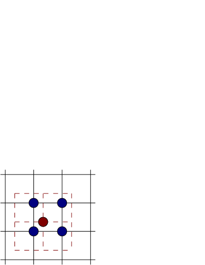
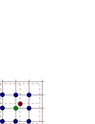
The “cloud-in-cell” (CIC) scheme uses the kernel factors

$$w_{\mathrm{CIC}}(\delta x)=\left\{\begin{array}[]{ll}1-|\delta x|/h&\mbox{for}\quad|\delta x|<h\\ 0&\mbox{otherwise}\end{array}\right.\;,$$ (19)

which implies that the particle is distributed over the four nearest grid points. A more elaborate scheme is the “triangular shaped cloud” (TSC) method, which uses the kernel factors

$$w_{\mathrm{TSC}}(x)=\left\{\begin{array}[]{ll}3/4-\delta x^{2}/h^{2}&\mbox{for}\quad|\delta x|\leq h/2\\ (3/2-|\delta x|/h)^{2}/2&\mbox{for}\quad h/2\leq|\delta x|<3h/2\\ 0&\mbox{otherwise}\end{array}\right.\;.$$ (20)

The CIC and TSC interpolation schemes are illustrated for two dimensions in Fig. 11. For all schemes, the kernel has to be normalised such that all particle mass fractions add up to unity.

Suppose now we have obtained the surface mass density on a grid $\kappa_{ij}=\kappa(\vec{x}_{ij})$, then the deflection angle can most straightforwardly be determined by direct summation as

$$\vec{\alpha}_{ij}=\frac{1}{\pi}\,\sum_{kl}\,\kappa_{kl}\,\frac{\vec{x}_{ij}-\vec{x}_{kl}}{\left|\vec{x}_{ij}-\vec{x}_{kl}\right|^{2}}\;.$$ (21)

Depending on the number of grid cells, the direct summation can be prohibitively slow. In many circumstances of astrophysical interest, fast-Fourier techniques can then be applied. In order to see how this works, note that the deflection angle can be written as a convolution of the convergence $\kappa(\vec{x})$ with a kernel

$$\vec{K}(\vec{x})=\frac{1}{\pi}\,\frac{\vec{x}}{\left|\vec{x}\right|^{2}}\;.$$ (22)

This allows the Fourier convolution theorem to be applied, which holds that the Fourier transform of a convolution is the product of the Fourier transforms of the functions to be convolved, hence

$$\hat{\vec{\alpha}}(\vec{k})=\hat{\kappa}(\vec{k})\hat{\vec{K}}(\vec{k})\;.$$ (23)

The Fourier transform of the kernel $\vec{K}$ can be determined and tabulated once. Using fast-Fourier techniques to determine the Fourier transform of the convergence $\hat{\kappa}(\vec{k})$ requires the convergence to be periodic on the lens plane. In many cases, this can be safely assumed or arranged. Often, lens planes are constructed from large-scale $N$-body simulations which have periodic boundary conditions by design, or the lens is an isolated object like a galaxy cluster, which can be surrounded by a sufficiently large field for the convergence to drop near zero everywhere around the edges of the field. Fast-Fourier methods speed up the computation of the deflection angle considerably.

If necessary, derivatives of the deflection angle field can also be determined in Fourier space. Once the convergence has been Fourier transformed, one can employ the two-dimensional Poisson equation to compute the Fourier transform of the lensing potential,

$$\hat{\psi}=-\frac{2}{k^{2}}\,\hat{\kappa}\;,$$ (24)

from which the Fourier transforms of the deflection angle and the shear components can easily be determined,

$$\hat{\vec{\alpha}}=-\mathrm{i}\,\vec{k}\,\hat{\psi}\;,\quad\hat{\gamma}_{1}=-\frac{1}{2}\left(k_{1}^{2}-k_{2}^{2}\right)\,\hat{\psi}\;,\quad\hat{\gamma}_{2}=-k_{1}k_{2}\,\hat{\psi}\;.$$ (25)

Relations like those and the exploitation of fast-Fourier methods are particularly relevant for simulating gravitational lensing by large-scale structures.

3 Lensing by Large-Scale Structures

3.1 Resolution Issues

Obviously, the thin-lens approximation that we have been using so far breaks down if one wishes to study gravitational lensing by large-scale structures. The solution then is to cover the complete cosmic volume whose lensing effects one wants to simulate with simulation boxes stacked along the line-of-sight, to project suitable slices on individual lens planes, and to use multiple lens-plane theory for describing light propagation.

The multiplicity of lens planes, and the general weakness of lensing by large-scale structures, make questions of angular and mass resolution particularly relevant for cosmic lensing. For instance, lens planes close to the observer are typically poorly resolved because even small grid cells span a large solid angle near the observer, and making grid cells smaller is not generally an acceptable solution because then the number of particles per grid cell becomes small, and the shot noise possibly unacceptably large. However, lens planes near the observer are less efficient than lens planes approximately half-way to the source because the lensing efficiency function is zero at the observer and source redshifts and peaks in between. Yet, structures grow over time, thus the lensing efficiency function is skewed towards lower redshifts because structures are geometrically less efficient lenses, but their density contrast keeps growing. By a related argument, sources at very high redshifts do not require the entire cosmological volume between them and the observer to be filled with lens planes because lens planes at very high redshift are geometrically inefficient and have a low density contrast. The left panel of Fig. 12 shows two examples for the lensing efficiency function times the linear growth factor, which is the relevant quantity combining structure growth with geometrical efficiency.

Figure 12: Left panel: The product of lensing efficiency function times the linear growth factor for density perturbations is shown for two different source redshifts, $z_{\mathrm{s}}=3$ and $z_{\mathrm{s}}=1000$, respectively, the latter being relevant for gravitational lensing of the cosmic microwave background. The growth factor skews the geometrical lensing efficiency towards lower redshifts. At redshift 5, the combined efficiency function drops to 10% of its peak value for $z_{\mathrm{s}}=1000$, implying that by far not the complete redshift range up to $z_{\mathrm{s}}$ needs to be covered with lens planes. Right panel: The solid curves show the rms cosmic convergence for sources at three different redshifts in per cent, the dashed curves the noise-to-signal ratio obtained in an $N$-body experiment with particle mass $m_{\mathrm{p}}=6.8\times 10^{10}\,h^{-1}\,M_{\odot}$. Both types of curve are plotted as functions of angular scale.

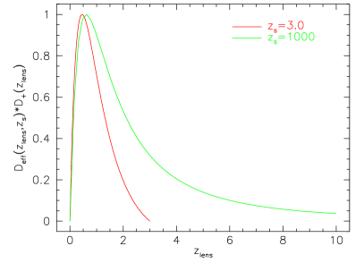
Similarly, the effective angular resolution of the simulation is dominated by the angular resolution of those lens planes near the peak in the combined efficiency function, i.e. the product of geometrical efficiency and linear growth factor.

The shot noise caused by the discretisation of mass into particles is particularly important for studies of weak lensing by large-scale structures. Even in absence of density inhomogeneities, shot noise leads to density fluctuations. They need to be sufficiently smaller than the signal, i.e. the convergence fluctuations which cause weak lensing.

In essence, this requirement also imposes a resolution limit. Suppose we wish to quantify the weak-lensing signal within a solid angle $\delta\Omega$. The volume spanned by $\delta\Omega$ within redshifts $z$ and $z+\mathrm{d}z$ is

$$\mathrm{d}V(z)=\delta\Omega\,D^{2}(z)\,\left|\frac{\mathrm{d}D_{\mathrm{prop}}}{\mathrm{d}z}\right|\,\mathrm{d}z\;,$$ (26)

where $D(z)$ and $D_{\mathrm{prop}}(z)$ are the angular diameter and proper distances to redshift $z$. In absence of density inhomogeneities, this volume element contains $\mathrm{d}N(z)$ particles, with

$$\mathrm{d}N(z)=\mathrm{d}V(z)\,\frac{\bar{\rho}(z)}{m_{\mathrm{p}}}\;,$$ (27)

where $\bar{\rho}(z)$ is the mean matter density at redshift $z$, and $m_{\mathrm{p}}$ is the mass of an $N$-body particle in the simulation. The contribution to the lensing convergence by these particles has to be weighted by the effective lensing distance, $D_{\mathrm{eff}}(z,z_{\mathrm{s}})$, and by numerical factors. Poisson fluctuations in the particle number thus cause convergence fluctuations whose variance is

$$\delta^{2}\kappa\propto\int_{0}^{z_{\mathrm{s}}}\mathrm{d}z\,D_{\mathrm{eff}}^{2}(z,z_{\mathrm{s}})\,\mathrm{d}N(z)\;.$$ (28)

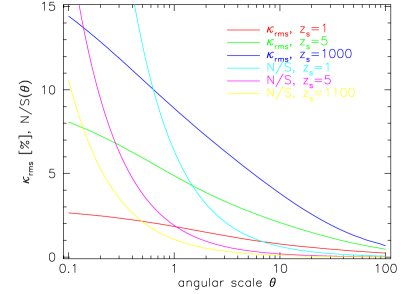
These fluctuations need to be compared with, and smaller than, the convergence fluctuations due to large-scale structure, which are typically of order $\langle\kappa^{2}\rangle^{1/2}\approx 5\%$ for sources near redshift unity and angular scales of order $1^{\prime}$. According to Eqs. (26) through (28), the rms shot noise $\langle\delta^{2}\kappa\rangle^{1/2}$ scales like $\delta\Omega^{1/2}$, thus the requirement that the signal-to-noise ratio

$$\frac{\mathrm{S}}{\mathrm{N}}=\left(\frac{\langle\kappa^{2}\rangle}{\langle\delta^{2}\kappa\rangle}\right)^{1/2}$$ (29)

exceed a specified threshold translates into a lower limit to the solid angle $\delta\Omega$ which can reasonably be resolved by the simulation. The smallness of the rms cosmic convergence $\kappa_{\mathrm{rms}}=\langle\kappa^{2}\rangle^{1/2}$ implies that many particles need to be enclosed by the “cone” spanned by $\delta\Omega$ for the simulation to be reliable. The right panel of Fig. 12 shows an example. The rms cosmic convergence in per cent and the noise-to-signal ratio are plotted as functions of angular scale. The noise level was adapted to an $N$-body simulation with particle mass $m_{\mathrm{p}}=6.8\times 10^{10}\,h^{-1}\,M_{\odot}$. The curves show that the noise-to-signal ratio drops below unity for sources at redshift $z_{\mathrm{s}}=1$ only if the angular resolution is lowered to $\gtrsim 5^{\prime}$, while an angular resolution of $\gtrsim 0.8^{\prime}$ can be achieved for $z_{\mathrm{s}}=1000$ (i.e. for weak lensing of the CMB; Pfrommer 2002).

3.2 Multiple Lens-Plane Theory

Weak lensing by large-scale structures requires the cosmic volume to be split into multiple lens planes rather than a single one (for general reference on multiple lens-plane theory, see Schneider et al. 1992). The lens plane closest to the observer is the image plane which represents the observer’s sky. A light ray piercing the image plane at a physical coordinate $\vec{\xi}_{1}$ is mutiply deflected on $N$ lens planes and finally reaches the source plane at the physical coordinate

$$\vec{\eta}(\vec{\xi}_{1})=\frac{D_{\mathrm{s}}}{D_{1}}\vec{\xi}_{1}+\sum_{i=1}^{N}\,D_{i\mathrm{s}}\,\vec{\hat{\alpha}}(\vec{\xi}_{i})\;,$$ (30)

where the $D_{i}$ and $D_{i\mathrm{s}}$ are the angular diameter distances from the observer to the $i$-the lens plane, and from the $i$-th lens plane to the source, respectively. The light ray passes the $i$-th plane at $\vec{\xi}_{i}$, where it is deflected by $\vec{\hat{\alpha}}(\vec{\xi}_{i})$. Similarly, the $\vec{\xi}_{i}$ are determined by

$$\vec{\xi}_{j}(\vec{\xi}_{1})=\frac{D_{j}}{D_{1}}\vec{\xi}_{1}+\sum_{i=1}^{j-1}\,D_{ij}\,\vec{\hat{\alpha}}(\vec{\xi}_{i})\;,$$ (31)

where $D_{ij}$ is the angular diameter distance from the $i$-th to the $j$-th lens plane.

Introducing angular coordinates $\vec{\theta}_{i}=\vec{\xi}_{i}/D_{i}$ yields

$$\vec{\theta}_{j}(\vec{\theta}_{1})=\vec{\theta}_{1}+\sum_{i=1}^{j-1}\,\frac{D_{ij}D_{\mathrm{s}}}{D_{j}D_{\mathrm{is}}}\,\vec{\alpha}(\vec{\theta}_{i})\;,$$ (32)

where we have introduced the reduced deflection angle $\vec{\alpha}=(D_{i\mathrm{s}}/D_{\mathrm{s}})\hat{\vec{\alpha}}$. We now define the matrices

$$\mathcal{A}_{i}=\frac{\partial\vec{\theta}_{i}}{\partial\vec{\theta}_{1}}\;,\quad\mathcal{U}_{i}=\frac{\partial\vec{\alpha}_{i}}{\partial\vec{\theta}_{i}}\;.$$ (33)

Clearly, $\mathcal{A}_{i}$ is the Jacobian matrix of the lens mapping between the $i$-th lens plane and the image plane, thus $\mathcal{A}_{N}$ is the Jacobian matrix of the mapping between the source and image planes. The goal is thus to determine $\mathcal{A}_{N}$ in order to obtain convergence, shear, and magnification for a light ray starting out into direction $\vec{\theta}_{1}$. The ray-tracing equation (32) implies the recursion relation

$$\mathcal{A}_{j}=\mathcal{I}-\sum_{i=1}^{j-1}\,\frac{D_{ij}D_{\mathrm{s}}}{D_{j}D_{\mathrm{is}}}\,\mathcal{U}_{i}\mathcal{A}_{i}\;,$$ (34)

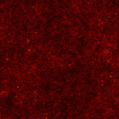
starting with $\mathcal{A}_{1}=\mathcal{I}$, the identity matrix. In summary, the deflection-angle fields $\vec{\alpha}_{i}$ on the $N$ lens planes can be used to construct the matrices $\mathcal{U}_{i}$ according to Eq. (33), then Eq. (34) can be used to determine the lensing experienced by a light ray starting out into any direction on the image plane. The left panel in Fig. 13 shows the total convergence experienced by sources at $z_{\mathrm{s}}=5$ on a lens plane with a side length of $4.25^{\circ}$, obtained from an $N$-body simulation (Pfrommer 2002).

Figure 13: Left panel: Effective convergence on a field of $4.25^{\circ}$ side length for sources at redshift $z_{\mathrm{s}}=5$, obtained using multiple lens plane theory on an $N$-body simulation. Right panel: Effective-convergence power spectra measured with the same set of simulations (crosses), compared with theoretical expectations (lines), for different source redshifts. The numerical results follow the theoretical curves very well within an intermediate range of wave numbers $l$. At larger $l$, i.e. for small structures, the resolution limit of the simulation is reached and the power spectra fall rather steeply. At the low-$l$ end, the noise increases because the number of modes in the simulation decreases as the modes increase. The numerical power spectra for low-redshift sources fall below the theroretical expectation at lower $l$ than for high-redshift sources because a given angle, and thus wave number $l$, corresponds to a larger physical scale at smaller distances from the observer (from Pfrommer 2002).

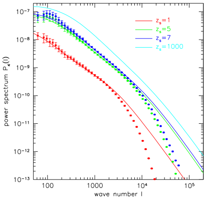
The right panel in Fig. 13 shows numerically determined power spectra for the effective convergence as functions of wave number $l$, which is the Fourier conjugate variable to the angular scale. The lines in this figure show the theoretically expected power spectra. The agreement between the numerical and theoretical results is very good over a limited range of wave numbers. Once the wave numbers increase beyond the limit set by the angular resolution, the simulated convergence fields lack power and the numerical results fall below the theoretical ones. This happens at lower $l$ for smaller source redshifts, because a fixed angular scale, and thus wave number $l$, corresponds to smaller physical scales at lower distances. On the low-$l$ end, i.e. for large structures, the errors on the numerically determined power spectra increase because the number of independent modes in the simulated convergence field decreases as the modes increase. This example should suffice to demonstrate that numerical simulations of gravitational lensing by large-scale structures should be carefully designed to match their final purpose.

4 Inversion Techniques

Let us conclude with a brief discussion of inversion techniques. They are typically less demanding numerically, but the methods which have been developed for this purpose are interesting in their own right.

4.1 Shear Deconvolution

We have seen before in Eqs. (24) and (25) that convergence and shear are related because they are both linear combinations of second derivatives of the scalar lensing potential $\psi$. In Fourier space, the relations are algebraic and can easily be combined to eliminate the Fourier transform $\hat{\psi}$ of the potential. Transforming back into configuration space, the convergence turns out to be a convolution of the shear with a well-known kernel,

$$\kappa(\vec{\theta})=\frac{1}{\pi}\,\int\mathrm{d}^{2}\theta^{\prime}\left[\mathcal{D}_{1}(\vec{\theta}-\vec{\theta}^{\prime})\gamma_{1}(\vec{\theta}^{\prime})+\mathcal{D}_{2}(\vec{\theta}-\vec{\theta}^{\prime})\gamma_{2}(\vec{\theta}^{\prime})\right]\;,$$ (35)

with

$$\mathcal{D}_{1}(\vec{\theta})=-\frac{\theta_{1}^{2}-\theta_{2}^{2}}{|\vec{\theta}|^{4}}\;,\quad\mathcal{D}_{2}(\vec{\theta})=-\frac{2\theta_{1}\theta_{2}}{|\vec{\theta}|^{4}}\;.$$ (36)

This is the classic Kaiser & Squires (1993) shear inversion equation. Its limitations have been discussed in detail and removed to satisfaction by modifying e.g. the kernel components $\mathcal{D}_{ij}$; they are not of interest for the discussion here (cf. Peter Schneider’s lecture in this volume).

A suitable practical approximation of (35) using measured galaxy ellipticities $\epsilon_{i}$ ($i=1,2$) is

$$\kappa(\theta)\approx\frac{1}{n\pi}\,\sum_{i=1}^{N}\left[\mathcal{D}_{1}\epsilon_{1,i}+\mathcal{D}_{2}\epsilon_{2,i}\right]\;,$$ (37)

where $n$ is the number density of lensed galaxies on the sky. In practice, however, it turns out that an approximation like (37) would have infinite noise because of the random sampling of the shear components $\gamma_{i}$ by $N$ galaxy ellipticities $\epsilon_{i}$. This can be remedied by introducing a smoothed kernel $\mathcal{D}^{\prime}$ instead of $\mathcal{D}$, e.g.

$$\mathcal{D}^{\prime}=\left[1-\left(1+\frac{\theta^{2}}{\theta_{\mathrm{s}}^{2}}\right)\exp\left(-\frac{\theta^{2}}{\theta_{\mathrm{s}}^{2}}\right)\right]\,\mathcal{D}\;,$$ (38)

where $\theta_{\mathrm{s}}$ is the angular smoothing scale (Seitz & Schneider 1995). The noise convariance matrix between the convergence values at two different grid points $\vec{\theta}_{i}$ and $\vec{\theta}_{j}$ is then

$$\left\langle\kappa(\vec{\theta}_{i})\kappa(\vec{\theta}_{j})\right\rangle=\frac{\sigma_{\epsilon}^{2}}{4\pi\theta_{\mathrm{s}}^{2}n}\,\exp\left[-\frac{(\vec{\theta}_{i}-\vec{\theta}_{j})^{2}}{2\theta_{\mathrm{s}}^{2}}\right]\;,$$ (39)

where $\sigma_{\epsilon}$ is the scatter of the intrinsic galaxy ellipticities (van Waerbeke 2000). This expression demonstrates that smoothing introduces correlations on the convergence map on the angular scale $\theta_{\mathrm{s}}$, but the variance of $\kappa$ can become very high if $\theta_{\mathrm{s}}$ is chosen too small. A careful balance between the local variance and non-local correlations is necessary in order to arrive at a convergence map with the required properties.

4.2 Maximum-Likelihood Lens Inversion

An entirely different approach to lens inversion uses the maximum-likelihood technique (Bartelmann et al. 1996). Each lensed background galaxy $i$ provides a measurement of two ellipticity components $(\epsilon_{1,i},\epsilon_{2,i})$ and its angular size. Comparing the size of a galaxy behind a galaxy cluster to the average size of unlensed galaxies of the same surface brightness, an estimate $r_{i}$ of the inverse magnification of the lensed galaxy can be derived. Thus $N$ galaxies provide a $3N$-dimensional data vector

$$\vec{d}=(\epsilon_{1,1},\epsilon_{2,1},r_{1},\ldots,\epsilon_{1,N},\epsilon_{2,N},r_{N})\;.$$ (40)

The goal of the lens inversion is then to find a two-dimensional array $\psi_{jk}$ of lensing potential values such that the ellipticities and inverse magnifications caused by that potential at the positions $\vec{\theta}_{i}$ of the real galaxies optimally reproduce the measured ellipticities and inverse magnifications. In other words, the potential values $\psi_{jk}$ have to be determined such as to minimise the mean-square difference between the data vector $\vec{d}$ and the model data vector $\vec{d}[\psi_{jk}(\vec{x}_{i})]$,

$$\chi^{2}(\psi_{jk})=\sum_{i=1}^{3N}\left\{\frac{[d_{i}-d_{i}(\psi_{jk})]^{2}}{\sigma_{i}^{2}}\right\}\;,$$ (41)

where the errors $\sigma_{i}$ can be estimated from the data themselves. The minimisation of $\chi^{2}$ with respect to the potential values $\psi_{jk}$ can be done with any minimisation algorithm like, e.g. the downhill simplex method. For large fields, the number of potential values can become very large. In that case, conjugate-gradient methods are preferred, which make use of the fact that the derivatives of $\chi^{2}$ with respect to the $\psi_{jk}$ are known analytically. Such methods can speed up the minimisation sufficiently to render it feasible even for large potential arrays (cf. Press et al. 1992).

4.3 Maximum-Entropy Methods

The minimisation of $\chi^{2}$ is a special case of the maximum-likelihood technique for assumed Gaussian deviations of the measured data around the model values. Improvements of the maximum-likelihood technique can be derived starting from Bayes’ theorem,

$$P(\psi|\vec{d})=\frac{P(\vec{d}|\psi)}{P(\vec{d})}\,P(\psi)\;,$$ (42)

which states that the probability $P(\psi|\vec{d})$ of finding the potential $\psi$ given the data $\vec{d}$ is proportional to the probability $P(\vec{d}|\psi)$ of obtaining the data given the potential, times the probability $P(\psi)$ for finding the potential. The denominator $P(\vec{d})$ is called the evidence and simply normalises Eq. (42). $P(\psi)$ is called the prior, quantifying any a priori information one has or assumes on the potential $\psi$, $P(\vec{d}|\psi)$ is called the likelihood, and $P(\psi|\vec{d})$ is the posterior probability. The goal is now to maximise the latter, which is equivalent to maximising the product $P(\vec{d}|\psi)\,P(\psi)$ of likelihood and prior. If we have or can assume Gaussian noise and a diagonal noise correlation matrix, the likelihood reduces to $P(\vec{d}|\psi)=\exp(-\chi^{2}/2)$.

It can now be shown that in absence of any further information, the best, i.e. least prejudiced, prior is the maximum-entropy prior,

$$P(\psi)\propto\exp\left[\alpha\,S(\psi,\vec{m})\right]\;,$$ (43)

with the cross entropy

$$S(\psi,\vec{m})=\sum_{i=1}^{3N}\,\psi_{i}-m_{i}-\psi_{i}\,\ln\frac{\psi_{i}}{m_{i}}\;,$$ (44)

where $\vec{m}$ is a model vector for the potential which can encode expectations on the potential, or simply be chosen to be uniform for all $i$. The potential array is then determined by maximising $\exp(-\chi^{2}/2+\alpha S)$, or equivalently by minimising

$$F\equiv\frac{1}{2}\chi^{2}-\alpha S$$ (45)

instead of the simple $\chi^{2}$ in Eq. (41). The parameter $\alpha$ can be included into the minimisation. Bayesian theory implies that a good approximation to the optimal choice for $\alpha$ is determined such that $F\sim 3N/2$ at the potential minimum $\bar{\psi}$. The error covariance matrix for the potential $\psi$ is given by the inverse curvature matrix of $F$,

$$\left\langle(\psi-\bar{\psi})(\psi-\bar{\psi})^{\mathrm{T}}\right\rangle\approx\left(\frac{\partial^{2}F}{\partial\psi_{i}\partial\psi_{j}}\right)^{-1}\;.$$ (46)

Maximum-entropy methods have been suggested and used for regularising shear-inversion techniques such that their spatial resolution is adapted to the strength of the lensing signal (Bridle et al. 1998; Seitz et al. 1998).

5 Concluding Remarks

Many numerical methods have been used for gravitational lensing studies which I was not able to cover during the limited time of the lecture. Among them are the hierarchical tree-code methods introduced into microlensing by Wambsganss et al. (1990) and the methods for constraining cluster mass distributions from multiple arc systems (e.g. Kneib et al. 1993; see also Jean-Paul Kneib’s presentation in this volume). Despite this unavoidable incompleteness, I hope to have given a flavour of how numerical methods can be used for lensing, and what the main problem areas are.