Relativistic Cosmology Number Counts
and the Luminosity Function

Abstract

This paper aims to connect the theory of relativistic cosmology number counts with the astronomical data, practice, and theory behind the galaxy luminosity function (LF). We treat galaxies as the building blocks of the Universe, but ignore most aspects of their internal structures by considering them as point sources. However, we do consider general morphological types in order to use data from galaxy redshift surveys, where some kind of morphological classification is adopted. We start with a general relativistic treatment for a general spacetime, not just for Friedmann-Lemaître-Robertson-Walker, of number counts, and then link the derived expressions with the LF definition adopted in observational cosmology. Then equations for differential number counts, the related relativistic density per source, and observed and total relativistic energy densities of the universe, and other related quantities are written in terms of the luminosity and selection functions. As an example of how these theoretical/observational relationships can be used, we apply them to test the LF parameters determined from the CNOC2 galaxy redshift survey, for consistency with the Einstein-de Sitter (EdS) cosmology, which they assume, for intermediate redshifts. We conclude that there is a general consistency for the tests we carried out, namely both the observed relativistic mass-energy density, and the observed relativistic mass-energy density per source, which is equivalent to differential number counts, in an EdS Universe. In addition, we find clear evidence of a large amount of hidden mass, as has been obvious from many earlier investigations. At the same time, we find that the CNOC2 LF give differential galaxy counts somewhat above the EdS predictions, indicating that this survey observes more galaxies at $0.1\>^{<}_{\sim}\>z\>^{<}_{\sim}\>0.4$ than the model’s predictions.

1 Introduction

In cosmology, it is one thing to obtain universe models from solutions of Einstein’s field equations, and quite another to express these solutions in terms of quantities and parameters which can be related directly to real astronomical observations. This intrinsic difficulty of cosmological research was perceived long ago by its practitioners, more or less by the time modern cosmology was launching its own foundations, in the 1920’s and early 1930’s. This perception initiated a process which led to the establishment of a division between theoreticians and observers, with the former being grouped in what may be termed as relativistic cosmology, usually considered to be the realm of the first task above, and the latter forming observational cosmology, which lies in the realm of the second one. Despite this division, there has always been a few, of course, who were able to link successfully these two sub-fields (e.g., Tolman 1934; McCrea 1934, 1939; Sandage 1961, 1995; Ellis 1971; Weinberg 1972; Ellis and Perry 1979; Ellis et al. 1984; Peebles 1980, 1993; Longair 1995). And more recently, there have been many individuals and groups of researchers who have successfully and closely linked cosmological observations (particularly those of the cosmic microwave background radiation and those involving deep galaxy surveys) to the standard Friedmann-Lemaître-Robertson-Walker (FLRW) theory. However, more needs to be done, particularly with regard to the broader issues of using observations to determine how good a model FLRW is on various cosmological length scales.

Each of these two approaches to cosmology (relativistic-theoretical and observational) has its own distinctive features. Relativistic cosmologists have been so successful in coping with the difficulties of obtaining exact solutions of Einstein’s field equations, that today one of the problems of this area is not the lack, but rather the excess, of solutions without the correspondent astrophysical modeling (Krasiński 1997). So, in relativistic cosmology a different cosmological model means in fact a different spacetime metric. Observational cosmologists, on the other hand, usually work almost exclusively with FLRW spacetimes, since, by its very nature, observational verification in cosmology is a formidable task, and since there are indications that the Universe is nearly FLRW on the largest scales. The fact that the characterization of FLRW geometry can be reduced to a set of a few parameters to be determined observationally, has allowed observational verification in cosmology to be reduced to manageable proportions. Or so it has been thought. Consequently, for observational cosmology a different cosmology often means, in fact, different parameter values for an FLRW spacetime metric, changing, for instance, its general topology from flat, to closed or open. Nevertheless, however different, these two sub-areas share the same general purpose of modern cosmology, which is to determine the spacetime geometry and the mass distribution of the Universe.

One of the most recent and comprehensive attempts to unify these two approaches in cosmology has been, perhaps, the ideal observational cosmology program, which proposes to characterize in detail the way in which cosmological observations can be directly used to determine the cosmological spacetime geometry (Ellis et al. 1985; Nel 1987). The main motivation behind this program has been to determine the spacetime metric of our universe directly from astronomical observations, without assuming a cosmological model beforehand (see Ellis, Matravers and Stoeger 1995). In the process of doing that, one must first determine what is and what is not decidable in cosmology on the basis of astronomical observations (Ellis et al. 1985, p. 317).

However, despite its obvious appeal, the ideal observational cosmology program still encounters a very basic problem: the astrophysical evolution, both in number and in luminosity, of galaxies, which are the fundamental astronomical makers of cosmic spacetime. Astrophysical evolution and cosmology are convolved in every presently practical astronomical observation of cosmological relevance. In order to implement the ideal observational cosmology program, not only do we require precise observations of redshift, galaxy number counts, and observer area distances (or luminosity distances), in the spherically symmetric case, but we also need an adequate model of how the populations and luminosities of the different types of galaxies evolve with redshift. It is presently impossible to determine this without assuming some cosmological model. This problem is so difficult that astronomers usually assume that the universe is well described by the standard FLRW geometry, and analyze, interpret and present their observational results in terms of that class of models, with or without a cosmological constant. On the largest scales – that is, on the largest scales probed by the cosmic microwave background radiation (CMBR) – there is good reason for doing this (see Stoeger, Maartens and Ellis 1995), although on scales less than these, this assumption is still in need of more adequate justification, inasmuch as we are incapable so far of determining the smallest length scale on which the FLRW approximation is valid. Thus, most observational results in cosmology either explicitly or implicitly assume an FLRW model in their presentation.

Although this approach has enabled the rapid progress of cosmology to this point, it may significantly hamper taking the next step: determining observationally how significant the deviations from FLRW are on various length scales, once we have some adequate model of galaxy evolution.

Finally, in some cases, in order to obtain simplified models, the approach taken in observational cosmology – particularly at low redshifts – has not been fully relativistic, and sometimes involves Euclidean simplifications, without proper verification of the limits within which such simplifications are justifiable (Ellis 1987; Ribeiro 2001). Though with the advent of much deeper surveys this is very rare now, it still causes some confusion, since some standard references show simplified presentations which, often for clarity, do not include these corrections.

The aim of this paper is to bridge the relativistic and observational cosmology approaches. But, it is much less ambitious than the ideal observational cosmology program, although we do intend to start with a fully relativistic approach and go as far as possible with the general equations, only then specializing them to particular geometries. In this paper, as an important example, we specialize to the Einstein-de Sitter model. The basic philosophy follows the general proposal for limited bandwidth observations of cosmological point sources outlined in Ribeiro (2002). However, our focus here will be on galaxy number counts, since this a very important cosmologically relevant quantity, giving information about the density of mass-energy in the universe, and can be determined by careful analysis of the data in galaxy redshift surveys. More particularly, therefore, our purpose is to present the detailed relationship between galaxy number counts, or galaxy luminosity functions, and relativistic mass-energy density and relativistic mass-energy density per source of the universe for any general cosmological model, and, as an example of how these relationships can be used, specialize them to FLRW and employ them to test the consistency of the FLRW model, in this case Einstein-de Sitter (EdS), assumed in deriving luminosity functions from a given redshift survey (the CNOC2 intermediate redshift survey) with the mass-energy density and mass-energy density per source, as functions of redshift, implied by that model. Do the number counts really determine these parameters to be EdS, as they should?

There are other ways, of course, in which we can use this framework. For instance, investigating the interplay of evolution, selection-effect and incompleteness models with various cosmologies in interpreting the same data, and testing simplifying and non-relativistic assumptions for certain redshift regimes. It should be mentioned here, too, that the other important cosmologically relevant observational parameter which complements number counts in determining the cosmological and evolution models is observer area distance (or luminosity distance). An scheme analogous to the one we present here for number counts can be established for this parameter (see Stoeger 1987; Stoeger and Araújo 1999).

Due to the reasons stated above, we shall in this paper specialize our model to FLRW. But we intend to expand this study eventually to non-FLRW metrics. This is justified because we wish to see what are the main differences between the predictions of reasonable non-FLRW metrics and those of the standard (FLRW) model. The only way we can really determine how good the Friedmann models are, is to fit almost-FLRW and non-FLRW models to the data, and compare them with the Friedmann fits to see if these latter are better (Ribeiro 2002). As the next logical step the obvious choice would be the Lemaître-Tolman-Bondi spacetime, since this is the most widely used metric for testing cosmological models after the standard model (Krasiński 1997).

Much of this detailed theoretical relativistic treatment has been presented before, but it was never linked or applied directly to luminosity function (LF) and number count data, with a careful discussion of the problems and obstacles of doing so. This is the first in a series of papers investigating how a fully rigorous general theoretical cosmological framework can effectively incorporate cosmologically relevant observational data – first assuming FLRW and testing for consistency, and then testing the FLRW hypothesis itself on various cosmologically relevant length scales by seeing if non-FLRW models also fit the data, with reasonable evolution, selection-effect and incompleteness assumptions.

As mentioned above, since most cosmological data is analyzed and presented employing the assumption of FLRW, we shall first perform consistency tests of the derived LF’s with the FLRW model they assume. Models with non-zero cosmological constant will be discussed in a follow-up paper (Stoeger and Ribeiro 2003)

The main conclusions we reach in this study is that the luminosity function parameters derived from data acquired by the recent redshift surveys are roughly consistent with the theoretical predictions of the standard Einstein-de Sitter (EdS) model. However, the relativistic energy density per source, or equivalently the galaxy number counts, departs from this model’s predictions at $0.1\>^{<}_{\sim}\>z\>^{<}_{\sim}\>0.4$. That may indicate either an inadequacy of the EdS cosmology to represent the data at those redshifts, or the rough number evolution model used in the CNOC2 LF calculations needs improvements.

This paper is organized as follows. In §2 we derive metric independent relations based on number source counting and the luminosity function. In §3 we collect the available data on the luminosity function and organize them in a form usable to our purposes. Section 4 specializes the general equations to the Einstein-de Sitter spacetime geometry, whereas section 5 carries out two consistency tests between the observational data and Einstein-de Sitter’s cosmological model theoretical predictions. Section 6 discusses the results and their implications.

2 Model Independent Counts of Cosmological Sources

We begin by deriving completely general cosmological number counting dependent quantities, which could, in principle, be determined directly from observations.

2.1 Relativistic Density of the Universe

2.1.1 Relativistic Number Counts

The key result derived by Ellis (1971) for the number of cosmological sources in a volume section at a point $P$ down the null cone is

$$dN=({d_{\scriptscriptstyle A}})^{2}d\Omega_{0}{\left[n\left(-k^{a}u_{a}\right)\right]}_{P}\;dy.$$ (1)

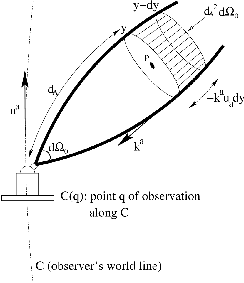
Figure 1: Section of a bundle of light rays subtending a solid angle $d\Omega_{0}$ as seen by the observer in $C(q)$. The affine parameter displacement $dy$ corresponds to a local distance variation of $\left(-k^{a}u_{a}\right)dy$ in the rest-frame of the galaxy at a point $P$ down the null cone (Ellis 1971).

Here $n$ is the number density of radiating sources per unit proper volume in a section of a bundle of light rays converging towards the observer and subtending a solid angle $d\Omega_{0}$ at the observer’s position, $d_{\scriptscriptstyle A}$ is the area distance  of this section from the observer’s viewpoint, $u^{a}$ is the observer’s 4-velocity, $k^{a}$ is the tangent vector along the light rays, and $y$ is the affine parameter distance down the light rays constituting the bundle (see figure 1). Notice that $n$ is measured in the rest-frame of the counted sources. This equation is metric independent, being, therefore, valid for all cosmological models (see Ellis 1971, p. 159 for more details). It should be noted that, in general, $n$ has a dependence both on the cosmology and on the number evolution of the sources. Only when the density of galaxies is constant in a comoving volume will $n$ be free of number evolution.

While the equation above is precise, it is written in terms of unobservable quantities, like the affine parameter $y$. It can be expressed in terms of observable quantities, but this has been previously done in observational coordinates, which are quite different from the usual ones (Ellis et al. 1985).

The general definition for the redshift can be written as (Ellis 1971, p. 146),

$$1+z=\frac{{\left[u^{a}k_{a}\right]}_{\mbox{\footnotesize source}}}{{\left[u^{a}k_{a}\right]}_{\mbox{\footnotesize observer}}}=\frac{{\left[u^{a}k_{a}\right]}_{P}}{{\left[u^{a}k_{a}\right]}_{C(q)}}.$$ (2)

Substituting equation (2) into equation (1) yields,

$$dN=({d_{\scriptscriptstyle A}})^{2}d\Omega_{0}{[n]}_{P}(1+z){\left[\left(-k^{a}u_{a}\right)\right]}_{c(q)}\;dy.$$ (3)

All the light rays reaching the observer’s worldline $C$ at the same time form a hypersurface which we call a past light cone, and which can be represented by a constant quantity over this surface. Following the notation of Ellis’ et al. (1985, p. 324), let us call the function generating this surface $w$. Therefore,

$$w=w(x^{a})=\mbox{const},$$ (4)

defines the past light cones along the observer’s worldline, the locus of light rays reaching the observer at a given moment of time. This constant is arbitrary, and we will choose it to be equal to the observer’s proper time $\tau$ at its worldline $C$. So, we may write the following equation,

$${\left[w(x^{a})\right]}_{C}={\left[\tau\right]}_{C}.$$ (5)

If we now define a vector field $k_{a}$, such that,

$$k_{a}\equiv-\frac{dw}{dx^{a}},$$ (6)

then this vector field generates past light cone surfaces. The minus sign was chosen because we are interested in incoming light rays, which are indeed geodesics of null type if their generating vector field obeys the following conditions (Ellis 1971; Ellis et al. 1985; Schneider et al. 1992, p. 94),

$$k^{a}k_{a}=0,\;\;\;{k^{a}}_{;b}k^{b}=0.$$ (7)

Now, using the definitions of $k_{a}$ and $u^{a}$, it follows that,

$$k_{a}u^{a}=-\frac{dw}{dx^{a}}\frac{dx^{a}}{d\tau}=-\frac{dw}{d\tau}.$$ (8)

Considering equation (5) we then conclude that,

$${\left[\frac{dw}{d\tau}\right]}_{C}=1,$$ (9)

and

$${\left[k_{a}u^{a}\right]}_{C}=-1.$$ (10)

This result allows us to write equation (3) as below,

$$dN=({d_{\scriptscriptstyle A}})^{2}(1+z)d\Omega_{0}\;n(y)\;dy.$$ (11)

This equation means that the local displacement at the rest-frame of the galaxy can be rewritten in terms of the redshift, as follows,

$$dl={\left[-u^{a}k_{a}\right]}_{P}\;dy=(1+z)dy.$$ (12)

We can actually write equation (11) completely in terms of $z$, with $n$ and ${d_{\scriptscriptstyle A}}$ as functions of $z$, since $z=z(y,\theta,\varphi)$. This is an important point to bear in mind, since in the next pages we will often refer to the quantity $dN/dz$, but rarely to $dN/dy$.

2.1.2 Average Galactic Mass

Although the number density of sources is very important for testing cosmological models, so is the mass-energy density of the universe. Thus, for completing our comparison of theory with observational data, we must at some stage relate mass-energy density to the number density of sources. To accomplish this we need to determine the average galaxy rest mass. At present this is not possible to determine from observations. So, let us indicate how it can be determined in principle, as well as discussing briefly the rough estimate we use here, for the sake of illustrating our general procedure.

Let us define ${\cal M}_{g}$ to be the average galaxy rest mass. Since galaxies of different morphological types may have masses varying from $10^{9}$ to $10^{12}$ solar masses, we may think of ${\cal M}_{g}$ as the simple average ${\cal M}_{g}=(1/V)\sum_{v=1}^{V}{\cal M}_{v}$, where $V$ is the number of galaxy morphological types being considered (ellipticals, spirals, irregulars, etc) and ${\cal M}_{v}$ is the typical rest-mass value for galaxies of a certain morphological class $v$. By “typical” we mean a simple average mass value. Note that this definition just takes the masses measured in nearby galaxies and extrapolates them to higher $z$.

Nonetheless, galactic class population abundances may vary with the redshift due to galaxy evolution, that is, galaxies may change from one morphological type to another in different epochs. In addition, galaxy rest masses are measured in the source’s rest frame. Furthermore, we may consider that some morphological types will be present only in certain redshift ranges, and be absent in others. Therefore, in general ${\cal M}_{v}$ will be a function of $z$, since the typical mass of a galaxy of a given type will vary with redshift. ${\cal M}_{v}(z)$ will still be an average of sorts – the average mass of, for instance, spiral galaxies in a redshift bin $\Delta z$. What ${\cal M}_{v}(z)$ is would have to be determined observationally and/or astrophysically, that is, with a combination of both observation and theory.

Considering this, it is therefore more appropriate to define ${\cal M}_{g}$ by means of the following weighted average,

$${\cal M}_{g}(z)=\sum_{v=1}^{V}P_{v}(z){\cal M}_{v}(z),$$ (13)

where $P_{v}$ is the galactic morphology population fraction, giving the abundance of each galactic type relative to the total number of counted galaxies in each redshift range. This quantity is normalized by

$$\sum_{v=1}^{V}P_{v}(z_{f})=1,$$ (14)

where $z_{f}$ stands for a fixed redshift value, or a certain redshift interval or bin $\Delta z$, to be determined observationally.

Equation (13) as defined above does not account for or describe galaxy mergers, as the basic information provided by it are the proportions of each galaxy population in the sample’s redshift range. However, it does allow for mergers when ${\cal M}_{g}(z)$ is considered together with the luminosity function (see §2.2 below). In the simplest possible case, we may assume just one morphological class ($V=1$), that, of course, will not change with the redshift, and its mass will be equal to the simple average of all galactic rest masses available. In this way equation (13) reduces to

$${\cal M}_{g}\approx 10^{11}{\cal M}_{\odot}.$$ (15)

Note again that this factor is just a rough estimate based on data presented by Sparke and Gallagher (2000, p. 204, 264; see their Table 5.1).

As stated above, we have written ${\cal M}_{v}(z)$ as a function of the redshift $z$, since galaxy interactions, including mergers, will affect the average galaxy masses of a given morphological type as the universe evolves. Similarly, $P_{v}(z)$ also depends on $z$ – as galaxies may change from morphological type to another as we go from earlier epochs to later ones. Typically, we find more spiral galaxies at higher redshifts, and more ellipticals at lower redshifts, for instance. But how are we to determine ${\cal M}_{v}(z)$? In principle, this can only be consistently done by using the galaxy luminosity functions for each type of galaxy as a function of redshift (which are defined and discussed below in §2.2), along some reliable measure of the masses of the galaxies in the sample – for instance the mass-to-luminosity ratio for them (see §2.4 below). Then, one could integrate the luminosity multiplied by the mass-to-luminosity ratio and the galaxy luminosity function over the luminosity, which is just the luminosity density convolved with the mass-to-luminosity ratio (see eq. 48 below), for each morphological type in a given redshift interval, to obtain the mass density contributed by that sample of galaxies. This can then be divided by the integral over the galaxy luminosity function itself for that particular type in the same redshift interval, giving the number density of galaxies of that type, to obtain the average galaxy mass for that sample. Perhaps, we shall eventually be able to do this. However, at present there are several problems. First of all, the luminosity functions diverge a the faint end, and it is not clear how to choose reliably a faint-end cutoff. There are a large number of dwarf galaxies, and we do not know where they cease in the luminosity function. Furthermore, we cannot reliably determine mass-to-luminosity ratios which will apply to the full range of galaxies in the samples.

Thus, converting galaxy number densities to mass-energy densities presents us with a serious problem. We plan to investigate how this might be done with some confidence in later work. For this paper, in order to illustrate our general methods, we simply set the values of the ${\cal M}_{v}(z)$ on the basis of the rough estimates for typical galaxies of given type $v$ as provided by Sparke and Gallagher (2000) and Elmegreen (1998). These values are given in §5, where we apply our two consistency tests. This is by no means adequate, but our focus in this paper is to illustrate how our general framework can be used, when we have enough reliable observational data.

2.1.3 Relativistic Density per Source

The number density of all cosmological sources in their own rest frames can be written as,

$$n(y)=\frac{\rho}{{\cal M}_{g}},$$ (16)

where $\rho$ is the local density as given by the right hand side of Einstein’s field equations. This presumes that the cosmological constant is zero, and that there is no dark matter not associated with the sources we are considering. If there is, then we can simply add those components to the matter density of the sources to obtain $\rho$. Now, following Stoeger et al. (1992, §3) we shall define the relativistic density per source ${\mu}(z)$ in terms of the differential number counts $dN/dz$ as

$${\mu}(z)\equiv\frac{{\cal M}_{g}}{{{(d_{\scriptscriptstyle A})}^{2}}d\Omega_{0}}\frac{dN}{dz}.$$ (17)

Thus, this quantity can, in principle, be determined observationally (Loh and Spillar 1986; Newman and Davis 2000). Remembering equation (11), we can also write $\mu(z)$ in terms of the cosmological density $\rho$,

$${\mu}(z)=(1+z)\;\rho\;\frac{dy}{dz}.$$ (18)

Interestingly, ${\mu}(z)$, or $dN/dz$, can be precisely determined theoretically for any cosmological model (e.g., for FLRW) and then compared with what is measured observationally (see below). In addition, one can clearly see that it is easier to find ${\mu}(z)$ from observations by means of equation (17), while it is easier to find ${\mu}(z)$ from theory by means of equation (18). It goes without saying, from what we have indicated above, that both ${\mu}(z)$ and $dN/dz$ depend on both cosmological evolution and astrophysical number evolution.

The relationship between the observed differential counts and the total count may be written as

$${\left(\frac{dN}{dz}\right)}_{0}=J\left(\frac{dN}{dz}\right),$$ (19)

where $J$ is the completeness parameter, giving the percentage of galaxies effectively observed in a galaxy redshift survey relative to the estimated total content of the sample. Thus,

$$0\leq J\leq 1,$$ (20)

and equation (17) becomes,

$${\mu}(z)=\frac{{\cal M}_{g}}{J{{(d_{\scriptscriptstyle A})}^{2}}d\Omega_{0}}{\left(\frac{dN}{dz}\right)}_{0}.$$ (21)

Notice that this equation is bolometric, since the observed differential count on the right side is not restricted to any pass-band wavelength observations. We can similarly write the observed relativistic density of the universe ${\mu}_{0}(z)$ in terms of the observed differential count as follows,

$${\mu}_{0}(z)=\frac{{\cal M}_{g}}{{{(d_{\scriptscriptstyle A})}^{2}}d\Omega_{0}}{\left(\frac{dN}{dz}\right)}_{0},$$ (22)

inasmuch as,

$${\mu}_{0}(z)=J{\mu}(z).$$ (23)

A final remark: although the equations above were written in terms of the area distance, expressions for the other observational distance definitions can be easily obtained by means of Etherington’s (1933) reciprocity theorem, valid for any cosmological metric. It may be written as follows (see also Ellis 1971, pp. 153-156; Schneider et al. 1992, pp. 110-114),

$$d_{\scriptscriptstyle L}=d_{\scriptscriptstyle A}{\left(1+z\right)}^{2}=d_{\scriptscriptstyle G}\left(1+z\right),$$ (24)

where $d_{\scriptscriptstyle L}$ is the usual luminosity distance, and $d_{\scriptscriptstyle G}$ is the galaxy area distance. The area distance is, in principle, an observationally determinable quantity, as its definition is given by (Ellis 1971, p. 153),

$${\left(d_{\scriptscriptstyle A}\right)}^{2}=\frac{dS_{0}}{d\Omega_{0}},$$ (25)

where $dS_{0}$ is the cross-sectional area at point $P$ of a bundle of null geodesics converging towards the observer (see figure 1). So, if, by means of some astrophysical model, we are able to infer the intrinsic cross-sectional area $dS_{0}$ of some object, and measure its subtended solid angle $d\Omega_{0}$, then $d_{\scriptscriptstyle A}$ can be found. Notice, however, that the cross-sectional area $dS_{0}$ is defined in the rest-frame of the source.

2.2 Galaxy Luminosity Function

The galaxy luminosity function $\phi$ is defined to be the local number density of all galaxies with absolute luminosity between $L$ and $L+dL$ at redshift $z$ (Weinberg 1972, p. 452; Peebles 1993, p. 119; Peacock 1999, p. 399),

$$\frac{dN(z,L)}{dV}=\phi(\ell)d\ell,$$ (26)

where

$$\ell\equiv L/L_{\ast},$$ (27)

$L_{\ast}$ is the luminosity scale parameter, and $dV$ is the proper volume element along the null cone, at some redshift, where the luminosity function is determined. Integration of $\phi$ above a certain luminosity threshold $L$ defines the selection function $\psi$ (Peebles 1993, p. 214),

$$\psi\left[\ell(z)\right]=\int_{\ell(z)}^{\infty}\phi(\ell)d\ell,$$ (28)

while summing $\phi$ over all luminosities yields,

$$\Psi(z)=\int_{0}^{\infty}\phi(\ell)d\ell.$$ (29)

This simplified formulation is an idealization. There is no universal galaxy luminosity function. In actuality, there are, instead, different luminosity functions for different types of galaxies and for different observational band-widths, and these evolve with redshift. Here we shall continue to let the unindexed luminosity function represent the distribution of all the galaxies, and designate the luminosity functions of certain classes of galaxies in certain observational band-width with subscript and superscript indices, respectively.

The introduction of the luminosity and selection functions means that in order to be detected and counted a galaxy must have a minimum flux, or apparent luminosity $F$, which is related to its intrinsic luminosity $L$, at some redshift $z$, by the well-known expression

$$F=\frac{L(z)}{4\pi{\left(d_{\scriptscriptstyle A}\right)}^{2}{\left(1+z\right)}^{4}},$$ (30)

for the case of bolometric flux. For a specific bandwidth range $W$, the apparent luminosity is further restricted to (Ellis 1971, p. 161; Ribeiro 2002),

$$F_{\scriptscriptstyle W}=\frac{L(z)}{4\pi{\left(d_{\scriptscriptstyle A}\right)}^{2}{\left(1+z\right)}^{3}}\int_{0}^{\infty}W(\nu){\cal J}\left[\nu(1+z)\right]d\nu,$$ (31)

where $W(\nu)$ defines the spectral interval of the observed flux (for instance, the standard UBV system) and ${\cal J}$ is the source spectrum function, that gives the proportion of radiation emitted by the source at some rest-frame frequency, but redshifted and detected by the observer as $\left[\nu(1+z)\right]$ (Ellis 1971, p. 161; Ribeiro 2002).

These two expressions for $F$ take into account relativistic effects. If those effects were to be left out, we would have to use their Euclidean counterparts, suitable for a non-expanding universe approximation. In this case the bolometric flux is given by,

$$F=\frac{L}{4\pi{\left(d_{\scriptscriptstyle L}\right)}^{2}},$$ (32)

which could also be found by using the reciprocity theorem (24) in equation (30). Similarly, the Euclidean equation for $F_{\scriptscriptstyle W}$ can also be found. Using the equation above for determining the luminosity function will strongly affect the galaxy counts, as the lower limit of the integral in equation (28) will be changed (Peebles 1993, p. 214).

The incompleteness of the sample is indicated by the lower limit of the integral in equation (28), since faint galaxies with intrinsic luminosity below $L(z)$ will not be counted. If we now suppose that the observationally determined luminosity function for brighter galaxies may also be used to account for those faint galaxies, we may then write the completeness parameter as,

$$J(z)=1-\frac{1}{\Psi(z)}\int_{0}^{\ell(z)}\phi(\ell)d\ell,$$ (33)

which agrees with condition (20), as it should. In addition, the selection function may be written as,

$$\psi\left[\ell(z)\right]=J(z)\Psi(z).$$ (34)

In order to provide a relativistic version for equation (26), we must link the definitions above to equation (11). However, it is clear from their definitions that the only difference between $n$, as in equations (1), (3) and (11), and $\phi$ is that the latter restricts the rest-frame volume count to a luminosity range. Considering this, we can only conclude that,

$$n(y)=\Psi\left[z(y)\right].$$ (35)

Notice that this equation assumes that both quantities above are measured relative to proper volume elements. If, however, $\Psi$ is being observationally determined by means of another volume definition, like the comoving volume, an appropriate conversion factor must be introduced in order for equation (35) be correct (see §4.3 below).

In addition, the functional relationship between the redshift $z$ and the affine parameter $y$ remains unknown in the general case, and must be determined by solving the field equations (in particular, the null Raychaudhuri equation). Thus, once a cosmological metric is assumed or specified, it can be determined. In other words, to fix the function $y=y(z)$ we require a cosmological solution of Einstein’s field equations. Of course, in practice we may be using some null radial coordinate other than the affine parameter, say $r$. Then we would need $r=r(z)$ or its inverse relationship. Below, in dealing with the Einstein-de Sitter cosmological model, we shall use an $r$ which is closely related to the radial coordinate which is often used in describing FLRW models.

We can write the relativistic number counts in terms of the luminosity function by substituting the result above into equation (11). The result yields,

$$dN={\left(d_{\scriptscriptstyle A}\right)}^{2}(1+z)d\Omega_{0}\Psi(y)dy.$$ (36)

Hence, the observed differential number counts for sources whose intrinsic luminosity are above the threshold $L(z)$ becomes,

$${\left[\frac{dN(z,>L)}{dz}\right]}_{0}={\left(d_{\scriptscriptstyle A}\right)}^{2}(1+z)d\Omega_{0}\;\psi\left[L(z)\right]\frac{dy}{dz},$$ (37)

while the total count yields,

$$\frac{dN(z)}{dz}={\left(d_{\scriptscriptstyle A}\right)}^{2}d\Omega_{0}(1+z)\Psi\frac{dy}{dz}.$$ (38)

The observed relativistic density per source in the universe will then be given by,

$${\mu}_{0}\left[z(y)\right]={\cal M}_{g}(1+z)\psi\frac{dy}{dz},$$ (39)

which implies that,

$$\rho={\cal M}_{g}\Psi,$$ (40)

if we assume the cosmological constant is zero and that all dark matter is associated with the sources. Otherwise, we would have to write $\rho_{m}={\cal M}_{g}\Psi,$ where $\rho_{m}$ represents only the matter associated with the sources themselves, not vacuum energy nor, for instance, matter distributed differently from the observed sources. These equations can be completely determined in terms of the redshift once the function $y=y(z)$ is found for a specific cosmological spacetime, allowing us to eliminate the affine parameter.

For bolometric counts the lower limit $L(z)$ is given by equation (30), while for counts in the bandwidth $W$ we must use equation (31). If observations are in a limited bandwidth $W$, then the observed relativistic density per source of the universe must be written as,

$${\mu}_{0}^{\scriptscriptstyle W}(z)=\sum_{v=1}^{V}P^{\scriptscriptstyle W}_{v}(z){\cal M}_{v}(z)J^{\scriptscriptstyle W}_{v}(z)(1+z)\Psi^{\scriptscriptstyle W}_{v}(z)\frac{dy}{dz},$$ (41)

where

$$\Psi^{\scriptscriptstyle W}_{v}(z)=\int_{0}^{\infty}\phi_{v}^{\scriptscriptstyle W}(\ell)d\ell,$$ (42)

and $J^{\scriptscriptstyle W}_{v}(z)$ is the completeness parameter determined by means of the bandwidth luminosity as given by equation (31), but with a luminosity function for each galaxy morphological type $v$ and at different wavebands $W$. Notice that since the luminosity function conveys observational information about the number of sources at each redshift bin, it will effectively take into account the possible galaxy mergers taking place in those ranges, with the morphological population fraction $P^{\scriptscriptstyle W}_{v}(z)$ conveying the observational relative abundance of each morphological type in the same redshift ranges, and for each observing bandwidth $W$. In other words, number evolution and cosmological evolution are contained in the luminosity function, but number evolution will also be reflected in ${\cal M}_{g}(z)$.

Remembering equation (23), the observed relativistic density per source can, for the best possible observations, be at most equal to its theoretical counterpart, ${\mu}_{0}(z)\leq{\mu}(z)$. However, if we now suppose the existence of some form of dark matter, we should rewrite equation (23), since the total theoretical value of ${\mu}$ should be given by the following expression,

$${\mu}(z)=\frac{{\mu}_{0}(z)}{J}+{\mu}_{d},$$ (43)

where ${\mu}_{d}$ accounts for the possible dark matter component. Therefore, from now on all theoretical quantities will be decomposed into an observational part, and a possibly unseen, differently distributed, component.

According to this definition, ${\mu}_{d}$ does not include dark matter galactic halos, as this is already included in the rest mass determination of each galaxy. So, ${\mu}_{d}$ may be baryonic intracluster dark matter, or non-baryonic dark matter, or vacuum energy, or still possibly, quintessence.

In writing ${\mu}_{0}(z)$ we have also to consider that it is composed by summing up the individual contributions of the different bandwidths $W$, $W^{\prime}$, etc, where the observations are actually made. Therefore, we have that,

$${\mu}_{0}(z)={\mu}_{0}^{W}+{\mu}_{0}^{W^{\prime}}+{\mu}_{0}^{W^{\prime\prime}}+\ldots$$ (44)

This equation is valid provided that the different bandwidths $W$, $W^{\prime}$, etc, do not overlap, otherwise there will be double counting. However, in general we may expect significant overlap of galaxy counts over different bandwidths, meaning that equation (44) will convey incorrect results due to overcounting of the galaxies we observe. In order to avoid this situation, let us rewrite equation (44) as follows,

$${\mu}_{0}(z)=\sum_{{\scriptscriptstyle W}=1}^{\scriptscriptstyle W_{f}}a_{\scriptscriptstyle W}(z){\mu}_{0}^{\scriptscriptstyle W}(z),$$ (45)

where

$$a_{\scriptscriptstyle W}(z)=1,\;\;\;\;\mbox{for}\;\;\;\;W=1,$$ (46)

and

$$a_{\scriptscriptstyle W}(z)=b_{\scriptscriptstyle W}(z)<1,\;\;\;\;\mbox{for}\;\;\;\;W>1.$$ (47)

Here $b_{\scriptscriptstyle W}(z)$ is the fraction of galaxies in waveband $W>1$ which are not counted in wavebands $1,2,\ldots,(W-1)$.

For later usage it is convenient to define the luminosity density as being given by (Peebles 1993, p. 120),

$$j=\int_{0}^{\infty}L\;\phi(\ell)d\ell.$$ (48)

This is the average luminosity of the sources per unit of proper or comoving volume.

2.3 Observed Average Densities

The observed average density of the universe is defined as follows,

$$\langle\rho\rangle\equiv\frac{{\cal M}_{g}N}{V_{0}},$$ (49)

where $V_{0}$ is the total observed volume. As discussed in Ribeiro (2001, and references therein), equation (49) does not define an unique quantity, but at least three, as the observational volume can be constructed with any of the three distance definitions given by the reciprocity theorem (24). Consequently, we have that

$$V_{0}\equiv\frac{4}{3}\pi{d_{0}}^{3},$$ (50)

where $d_{0}$ may be any of the three distances, $d_{\scriptscriptstyle L}$, $d_{\scriptscriptstyle A}$, or $d_{\scriptscriptstyle G}$. As at the observer’s position $C(q)$ the redshift is zero, these definitions must imply that

$$\lim_{z\rightarrow 0}\langle\rho\rangle=\rho_{0}.$$ (51)

Notice that the observational quantities so far used, namely $n$, and $\phi$, are not average densities, but local densities, defined at the source’s rest frame.

To determine $\langle\rho\rangle$ the key quantity to be found is $N$. Bearing in mind the results previously derived, the number of observed sources above a certain luminosity $L(z)$ is given by,

$$N_{0}(z,>L)=\sum_{{\scriptscriptstyle W}=1}^{\scriptscriptstyle W_{f}}a_{\scriptscriptstyle W}(z)N_{0}^{\scriptscriptstyle W}(z)=\sum_{{\scriptscriptstyle W}=1}^{\scriptscriptstyle W_{f}}a_{\scriptscriptstyle W}\int_{0}^{y}{\left(d_{\scriptscriptstyle A}\right)}^{2}(1+z)\;d\Omega_{0}\;{J^{\scriptscriptstyle W}}\;\Psi^{\scriptscriptstyle W}\;dy,$$ (52)

while the overall number of sources of any luminosity is,

$$N(z)=\sum_{{\scriptscriptstyle W}=1}^{\scriptscriptstyle W_{f}}a_{\scriptscriptstyle W}(z)N^{\scriptscriptstyle W}(z)=\sum_{{\scriptscriptstyle W}=1}^{\scriptscriptstyle W_{f}}a_{\scriptscriptstyle W}\int_{0}^{y}{\left(d_{\scriptscriptstyle A}\right)}^{2}(1+z)\;d\Omega_{0}\;\Psi^{\scriptscriptstyle W}\;dy.$$ (53)

We can now write the observed and total average densities of the universe in terms of the previously defined quantities. The expressions yield,

$${\langle\rho\rangle}_{0}=\frac{3}{4\pi{\left(d_{0}\right)}^{3}}\sum_{{\scriptscriptstyle W}=1}^{\scriptscriptstyle W_{f}}a_{\scriptscriptstyle W}(z)\sum_{v=1}^{V}{P^{\scriptscriptstyle W}_{v}(z){\cal M}_{v}(z)}\int_{0}^{y}{\left(d_{\scriptscriptstyle A}\right)}^{2}(1+z)\;d\Omega_{0}\;\psi_{v}^{\scriptscriptstyle W}\;dy,$$ (54)

and

$$\langle\rho\rangle={\langle\rho\rangle}_{d}+\frac{3}{4\pi{\left(d_{0}\right)}^{3}}\sum_{{\scriptscriptstyle W}=1}^{\scriptscriptstyle W_{f}}a_{\scriptscriptstyle W}(z)\sum_{v=1}^{V}{P^{\scriptscriptstyle W}_{v}(z){\cal M}_{v}(z)}\int_{0}^{y}{\left(d_{\scriptscriptstyle A}\right)}^{2}(1+z)\;d\Omega_{0}\;\Psi_{v}^{\scriptscriptstyle W}\;dy,$$ (55)

where ${\langle\rho\rangle}_{d}$ is the possible dark matter component. In redshift bins where $\phi$ varies little with $z$, we have the following result,

$${\langle\rho\rangle}_{0}=J{\langle\rho\rangle}-{\langle\rho\rangle}_{d}.$$ (56)

It is clear from equations (54) and (55) that building an average density from observations is a very complex task which depends on many choices, like the appropriate distance definitions to be used, and a still to be determined function $y=y(z)$ (if we do not assume a cosmology to begin with), which is certain to be non-linear. In addition, the complexity and high non-linearity of $\langle\rho\rangle$ shows the inherent difficulties of the task of observationally ascertaining whether or not the universe is smooth when one follows a fully relativistic approach of this problem (Ribeiro 2001).

2.4 Mass-to-Luminosity Ratio

The mass-to-luminosity ratio at some redshift depth is defined as,

$${\cal M}/L\equiv\frac{\rho}{j}={\cal M}_{g}\frac{\Psi}{j},$$ (57)

while its observable counterpart is given by,

$${\left[{\cal M}/L\right]}_{0}={\cal M}_{g}\frac{\psi}{j}.$$ (58)

If the average luminosity of the universe is similarly defined as the average density $\langle\rho\rangle$, we have that,

$$\langle j\rangle=\frac{L_{g}N}{V_{0}},$$ (59)

where $L_{g}$ is the average galaxy luminosity, given by

$$L_{g}(z)=\sum_{v=1}^{V}P_{v}(z)L_{v}(z).$$ (60)

Here $L_{v}$ is the typical luminosity value for galaxies of a certain morphological type $v$, and $P_{v}$ is the galactic fractional population class (see eqs. 13 and 14).

From the equations above, the average mass-to-luminosity ratio at some redshift depth is given by,

$$\langle{\cal M}/L\rangle=\langle\rho/j\rangle=\frac{\langle\rho\rangle}{\langle j\rangle}=\frac{{\langle\rho\rangle}_{0}}{{\langle j\rangle}_{0}}=\frac{\sum_{v=1}^{V}P_{v}(z){\cal M}_{v}(z)}{\sum_{v=1}^{V}P_{v}(z)L_{v}(z)}.$$ (61)

3 Luminosity Function Data

The discussion presented so far has focused on galaxy number counts, which, aside from the redshift, is one of the two observational quantities (observer area distance, or luminosity distance is the other) which determine the geometry and mass-energy distribution of the Universe (assuming spherical symmetry - if this is not assumed, then we need two other quantities, cosmological proper motions and null shear parameters - see Ellis et al. 1985). Thus, the ideal way to determine the mass-energy distribution and the geometry would be by solving the field equations directly with redshift, number count and observer area distance data. However, as already mentioned, our ignorance of luminosity and number evolution, and adequate model of which would have to be assumed, is an obstacle to implementing this in a compelling way. Because of this, and since the luminosity functions available in the literature presuppose a definite FLRW cosmology, the first and easiest sensible application of the general theory we have summarized above is to test luminosity functions for consistency with observational relationships determined by the cosmologies they have assumed. In other words, in any specific cosmological metric we need to make both sides of the equation

[geometric cosmological model] $\leftrightarrow$ [parameterized data]

consistent, as we will be dealing either with quantities which are determined only observationally (e.g., $\phi$), or with theoretical quantities derived from the chosen cosmological model (e.g., ${\mu}$, $N$), or both (e.g., $dN/dz$, ${\cal M}/L$) (Stoeger 1987, p. 299).

The luminosity function provides an excellent observational tool for testing cosmological models, as it conveys information on how the local number of galaxies $n$ vary for different types of galaxies, its environmental dependence, how $n$ changes with the cosmic epoch (see eq. 35), and also a possible indirect estimate of the amount of dark energy present. The luminosity functions also provide a statistical description of the galaxy population. The functional form of $\phi$ and its parameter values are extracted from magnitude-limited redshift surveys of galaxies by means of various statistical techniques (Peebles 1993, p. 119; Binney and Merrifield 1998, p. 162; Peacock 1999, §13.3). Here, however, we shall only be interested in collecting from the literature the shape, normalization, and the luminosity scale of $\phi$ for the purpose of using it in our equations for the mass-energy density and the relativistic mass-energy density per source, and checking that the results are consistent with the cosmology assumed in calculating the luminosity functions. Some of the information contained in the luminosity functions is tied to the galaxy morphological or spectral class (see below), which means that at least a simplified morphological division must be assumed.

As discussed by Chen et al. (2001), various deep redshift surveys have yielded consistent measurements of the luminosity function for galaxies at $z\>^{<}_{\sim}\>0.75$ (Marzke et al. 1998; Lin et al. 1999; Cole et al. 2001), and this is precisely the redshift depth we are interested in here (see §1). Impey and Bothun (1997) have also compiled valuable observational data on $\phi$. Since these studies yield recent data on $\phi$, they seem reliable for giving the luminosity functions for this redshift range.

3.1 Morphological Types

As it is well known, galaxies have different morphologies, which vary from ellipticals and spheroidals to spirals and irregularly shaped galaxies (Binney and Merrifield 1998, ch. 4; Elmegreen 1998, ch. 2; Sparke and Gallagher 2000, §1.3). Redshift surveys dealing with thousands of galaxies tend, however, to automatically classify galaxies according to their spectral energy distributions (Lin et al. 1999, p. 539; Cole et al. 2001, §5.3), or by means of a simple three-type scheme, as E/S0, spiral, and irregular/peculiar galaxies (Marzke et al. 1998). It is important to mention that spectral type classifications are not necessarily straightforwardly related to the galaxy types of the Hubble diagram, and its extensions, and, since many surveys do adopt such a scheme, for the purposes of this paper it seems enough to follow Lin’s et al. (1999) spectral morphological types. So, from now on we will assume $V=3$ (see eq. 13), for three loose classification types: $v=1$ stands for early type galaxies, roughly E/S0; $v=2$ accounts for intermediate type galaxies, something like Sa-Sb; and $v=3$ represents late type galaxies, which would be Sc-I types. Notice, again, that this equivalence between the galactic spectral energy distributions and morphological types is not strict, and, therefore, should not be taken as giving a precise classification.

The classification scheme above is not unique. For instance, with the data presented by Impey and Bothun (1997) one could think of only two galactic types: $v=1$ for galaxies in clusters, which tend to be dominated by spirals, and $v=2$ for field galaxies, which are usually ellipticals. One could even think of other classification schemes, like luminous galaxies ($v=1$), low surface brightness galaxies ($v=2$), and luminous giants galaxies ($v=3$), or still $v=1$ for red galaxies, and blue galaxies as $v=2$. Perhaps, combinations of all these schemes are possible, although in such a case the problem of overcounting could become more acute.

Nevertheless, whatever classification scheme is chosen when applying the theory developed above, the bottom line is that the adopted morphological types will be dependent basically on the sample, or on the sampling method, used in the chosen redshift survey. In most cases it will probably not involve strict identification with the galaxy morphologies of the Hubble diagram. So, from now on the term “morphological type” will have a broad meaning, referring to some sort of classification obtained by differentiating the galaxies contained within a certain sample. Such a classification can be based either on spectra, or on the galactic shapes as given by the Hubble diagram, or on any other galactic observational feature considered important by some sampling method.

3.2 Shape

In finding the shape of the luminosity function, most, if not all, recent redshift surveys fit their data by using Schechter’s (1976) elegant form, which summarized earlier findings by Zwicky and Abell that the luminosity function is a broken power law, $\phi\sim L^{-1.5}$ at $L<L_{\ast}$, bending to $\phi\sim L^{-3}$ at the bright end (Peebles 1993, p. 119). Schechter’s luminosity function is given by,

$$\phi(\ell)=\phi_{\ast}\;\ell^{\alpha}e^{-\ell},$$ (62)

where $\phi_{\ast}$ characterizes the space density of galaxies, and $\alpha$ is the asymptotic slope of the faint end of the luminosity function. The luminosity scale $L_{\ast}$ is given in $\ell$ (see eq. 27), and tells us the luminosity above which galaxies are rare. These three constants are all observationally determined parameters.

The power law index $\alpha$ for the faint end slope is part of the shape determination of the luminosity function, and, according to the latest observations, it does change with the morphological class of the surveyed galaxies, whether they are field galaxies, dwarfs, giants, spiral-rich galaxy clusters, luminous galaxies or low surface brightness galaxies (Impey and Bothun 1997). The analytical form of equation (62), however, does not appear to vary with galactic properties. Only the values of the parameters do.

In the early days of the work on the luminosity function, all parameters were fitted to data only for local galaxies, where evolution is not considered to be important. However, as the surveys went deeper and deeper it became clear that possible luminosity evolution had to be taken into account. This can be done by allowing some of the fitted parameters to vary with the redshift (Lin et al. 1999), or by comparing their values at different redshift bins (Chen et al. 2001). Obviously, a great deal of work is needed to model luminosity and number evolution accurately, such as that pioneered by Totani, Yoshii, and their collaborators (Totani and Yoshii 2000; Totani et al. 2001). We are not concerned in this paper with doing this. In order to illustrate how our framework can be used, we provisionally accept the rough evolutionary models assumed in the CNOC2 survey and test them for cosmological consistency (see below).

3.3 Normalization and Luminosity Scale

Once the shape is determined, which includes determination of the faint-end slope, that is, the $\alpha$ parameter, we are still left with two unknowns, the normalization factor $\phi_{\ast}$ and the luminosity scale $L_{\ast}$. Various determinations of $\phi_{\ast}$ show it not to be very sensitive to different FLRW models, even to those with non-zero cosmological constant, meaning that up to $z\approx 1$ these measurements appear to be robust. The same seems also true for $\alpha$ and $L_{\ast}$. The major differences in these quantities seem to come from measurements of different morphological types and in different bandwidths (Binney and Merrifield 1998, p. 167; Lin et al. 1999; Cole et al. 2001). So, the present data seems to indicate only a weak dependence of these parameters on the cosmological models (Cross et al. 2001).

Redshift surveys usually present the fitted $L_{\ast}$ parameter in terms of its characteristic absolute magnitude $M_{\ast}$. So, in order to use these we have to rewrite equation (26) for the luminosity function as the number density of all galaxies between absolute magnitudes $M$ and $M+dM$. For Schechter’s form (62) that becomes (Binney and Merrifield 1998, p. 163),

$$\phi(\ell)\;d\ell=\phi_{\ast}\;\ell^{\alpha}e^{-\ell}d\ell=\left(0.4\ln 10\right)\phi_{\ast}10^{0.4\left(1+\alpha\right)\left(M_{\ast}-M\right)}\exp\left[-10^{0.4\left(M_{\ast}-M\right)}\right]dM=\phi(M)\;dM,$$ (63)

since the definition of absolute magnitude implies that $\ell=10^{0.4(M_{\ast}-M)}$.

3.4 The CNOC2 Redshift Survey Data

We have chosen to extract data to be used here from the Canadian Network for Observational Cosmology Field Galaxy Redshift Survey (CNOC2), presently the largest such a sample at intermediate redshifts. The CNOC2 sample for luminosity function (LF) determination contains over 2000 galaxies in the range $0.12<z<0.55$, and with apparent magnitude in the red band within $17.0<R_{c}<21.5$. Their fitting parameters were confirmed at $z\sim 0.75$ (Lin et al. 1999; see also Chen et al. 2001). The authors also claim their fitting to be valid with little difference for $0<z<1$. CNOC2 data were obtained and fitted in three bandwidths, $B_{\scriptscriptstyle AB}$, $R_{c}$, and $U$, and are available for FLRW models with $q_{0}=0.5$ and $q_{0}=0.1$. Therefore, by providing data in the redshift range we are interested in for different bandwidths, and presupposing the Einstein-de Sitter cosmological model, the CNOC2 survey is the most suitable to exemplify how we can use this theoretical-observational framework for testing the consistency of the LF’s with the assumed cosmology, for determining how much dark matter there is distributed differently than what is assumed associated with galaxies, and for eventually determining the range of validity of simplifying assumptions at low redshifts, among other things.

The required data for the CNOC2 LF’s assuming EdS universe are summarized in the tables 1, 2, and 3, where $v$ denotes the three morphological types in which the sample population is divided: early, intermediate and late spectral types (see §3.1 above), and $P_{v}$ the proportion of each galaxy population as compared to the whole sample. This is a fixed value in all CNOC2 redshift range. $M_{\ast}^{\prime}$ and $Q$ are two constants of the linear equation for the characteristic luminosity scale evolution (Lin et al. 1999, §3.2),

$$M_{\ast}(z)=M_{\ast}^{\prime}-Q(z-0.3),$$ (64)

and $\phi_{\ast}$ is in units of h³ Mpc^-3 mag^-1.

In computing these parameters of the LF from the CNOC2 survey, it is important to note that Lin et al. (1999) also adopted a model for galaxy number density evolution and assumed that the parameter $\alpha$, which governed the shape of the LF at the faint end, does not change with redshift for a given morphological type. They were also careful to consider surface density selection effects, and estimate the incompleteness of their sample, especially at the higher end of their redshift range. Finally, they performed various consistency checks to make sure that the LF parameters derived adequately represent the data for the redshifts indicated. It is reassuring that Cohen (2002) finds that her results for the Caltech Faint Galaxy Redshift Survey agree very well with the CNOC2 results, including for the faint-end slope of the LF’s. Similarly, the results from the Deep Groth Strip Survey (Im et al. 2002) are in agreement with the CNOC2 results, especially for the luminosity evolution parameter $Q$. The one discrepancy that has emerged is that the significant number evolution for late-type galaxies in the CNOC2 results is not found by either Cohen (2002) or Im et al. (2002). Im et al. (2002) speculate that this may be due to the fact that the CNOC2 samples were selected purely by colors. This means at low redshifts ($z<0.4$), where the difference in colors for various galaxy types is small, photometric errors can easily bump blue galaxies into the red-galaxy samples. Other than this, the CNOC2 LF results seem well supported for this redshift range.

The determination of the LF’s with CNOC2 data employed the comoving volume instead of the proper volume (Huan Lin 2002, private communication). Therefore, to be usable for us here we must apply an appropriate volume conversion factor to the results listed in tables 1-3 (see §4.3 below).

4 CNOC2 and Einstein-de Sitter

As already mentioned, we now want to use our observational-theoretical framework first to test the consistency of the CNOC2 LF results with the cosmological model it assumes, which is EdS. This has the added advantage that EdS is mathematically the simplest of the FLRW models. Furthermore, it is a frequently used case in the LF’s available in the literature. The extension of this type of analysis to other more general FLRW cosmologies, including those with a non-zero cosmological constant, are the subject of a forthcoming paper (Stoeger and Ribeiro 2003).

4.1 The Metric

Let us write the EdS metric as follows $(c=G=1)$,

$$ds^{2}=dt^{2}-a^{2}(t)\left[dr^{2}+r^{2}\left(d\theta^{2}+\sin^{2}\theta d\varphi^{2}\right)\right],$$ (65)

where $a(t)$ is the scale factor, given by

$$a(t)={\left(t+\frac{2}{3H_{0}}\right)}^{2/3},$$ (66)

$H_{0}$ is the Hubble constant, and the local density is

$$\rho=\frac{1}{6\pi a^{3}(t)}.$$ (67)

The solution of the past light cone equation, $dt/dy=-a(t)dr/dy$, may be written as,

$$3{\left[t(y)+\frac{2}{3H_{0}}\right]}^{1/3}={\left(\frac{18}{H_{0}}\right)}^{1/3}-r(y),$$ (68)

which allows us to write equation (66) along the null cone parameterized by $r$, as follows,

$$a[t(r)]=\frac{1}{9}{\left[{\left(\frac{18}{H_{0}}\right)}^{1/3}-r\right]}^{2}.$$ (69)

Detailed calculations on this spacetime along the lines followed in this article are widely available (see, for instance, Ribeiro 1995, 2001). Therefore, here we will only summarize some important results required in what follows.

4.2 Observables

Equations (66) and (69) allow us to obtain the function $z=z[r(y)]$, that is, an expression for the redshift where the affine parameter becomes implicit. In EdS it may be written as,

$$1+z=\frac{a(t=0)}{a(t)}={\left(\frac{18}{H_{0}}\right)}^{2/3}{\left[{\left(\frac{18}{H_{0}}\right)}^{1/3}-r\right]}^{-2}.$$ (70)

Applying equation (25) to the metric (65) gives us the area distance in this cosmology, which, by means of equation (70), yields,

$$d_{\scriptscriptstyle A}=ra(t)=\frac{2}{H_{0}}\left[\frac{\sqrt{1+z}-1}{{\left(1+z\right)}^{3/2}}\right],$$ (71)

since along the past null cone the scale factor may be written as,

$$a={\left(\frac{18}{H_{0}}\right)}^{2/3}\frac{1}{9{\left(1+z\right)}}.$$ (72)

In EdS geometry, for comoving sources, $u^{b}=\delta^{b}_{0}$, we have that,

$$-k^{b}u_{b}=-k^{b}g_{0b}=-k^{0}=-dt/dy=a(dr/dy),$$ (73)

which substituted into equation (1), and also remembering equation (16), gives us the total relativistic density per source (17) in the Einstein-de Sitter cosmology, as written below,

$${\mu}(z)=\frac{{\cal M}_{g}}{{\left(d_{\scriptscriptstyle A}\right)}^{2}d\Omega_{0}}\frac{dN}{dz}=\frac{3H_{0}}{8\pi}\sqrt{1+z}.$$ (74)

From these expressions, the results below readily follow.

$$\frac{dN}{dz}=\frac{3d\Omega_{0}}{2\pi H_{0}{\cal M}_{g}}\frac{{\left(\sqrt{1+z}-1\right)}^{2}}{{\left(1+z\right)}^{5/2}},$$ (75)

$$N(z)=\frac{d\Omega_{0}}{\pi H_{0}{\cal M}_{g}}{\left(1-\frac{1}{\sqrt{1+z}}\right)}^{3},$$ (76)

$$\rho(z)=\frac{3{H_{0}}^{2}}{8\pi}{\left(1+z\right)}^{3}.$$ (77)

Finally, with either equations (18) and (74), or (11) and (75), we can calculate the relationship between the affine parameter and the redshift in this cosmology. It may be written as follows,

$$\frac{dy}{dz}=\frac{1}{H_{0}{\left(1+z\right)}^{7/2}}.$$ (78)

4.3 Volumes

Before we proceed with the tests, there is one more issue to be taken care of: volume definitions. This is a tricky issue in relativistic cosmology as in general relativity volumes are not uniquely definable quantities, and they may vary quite substantially from one another even at $z\approx 0.1$ (Ribeiro 2001). Therefore, to avoid confusion, let us state clearly what volume definitions we have been using.

Equation (35) states that both the luminosity function and number density are defined using local volumes, that is, volume elements defined at the rest-frame of a galaxy at a given redshift $z$. From equations (11) and (12) it is clear that this volume is given by the following expression,

$$dV_{\rm local}=dl.dS_{0}=(1+z)dy{\left(d_{\scriptscriptstyle A}\right)}^{2}d\Omega_{0}.$$ (79)

Considering equation (78) it follows that in EdS cosmology this reduces to,

$$dV_{\rm local}={\left(d_{\scriptscriptstyle A}\right)}^{2}d\Omega_{0}\frac{dz}{H_{0}{(1+z)}^{5/2}}.$$ (80)

Sometimes observers refer to their data being reduced against the real, or proper volume, obtained by means of the spatial portion of metric (65), as follows,

$$dV_{\rm proper}=a^{3}r^{2}dr\sin\theta d\theta d\varphi.$$ (81)

Remembering equations (70) and (71), one can easily show that proper and local volumes, that is, equations (80) and (81), are equal. Nevertheless, we believe that since both the luminosity function and number density are defined locally, it makes more conceptual sense to refer to the local volume, as given by equations (79) and (80). In addition, it is important to stress that the local and proper volumes are in general not equal to the observed volumes defined by equation (50), as observed volumes use the three observational distances given by the reciprocity theorem (24).

When carrying out their data reduction, observers also used to refer to a survey volume, defined as (Sandage et al. 1979),

$$V_{\rm survey}=\frac{1}{3}d\Omega_{0}{\left(\frac{{\cal U}_{\rm max}}{H_{0}}\right)}^{3},$$ (82)

where ${\cal U}_{\rm max}$ is the maximum velocity obtained in the survey, being calculated by means of the Doppler velocity-redshift approximation ${\cal U}=cz$, valid only for small $z$. As it is well known, it is only under this approximation that we can write the redshift-distance law, that is, the Hubble law, as a velocity-distance law (Harrison 1993), since the velocity-distance law is a general result of an isotropic homogeneous expanding universe, whereas the redshift-distance law is a mere approximation of the form, valid at small redshift. That, in turn allows us to obtain the survey volume. Such a procedure not only employs the low redshift approximation, but also implicitly assumes the redshift distance $d_{z}$ as the distance definition used in $V_{\rm survey}$ (see footnote at page 7). Therefore, if one follows this path, model independent observable distances, like $d_{\scriptscriptstyle A}$ or $d_{\scriptscriptstyle L}$, are related to $d_{z}$ only in an approximate manner in EdS cosmological model, $d_{z}$ approximately scales only with $d_{\scriptscriptstyle L}$, in addition to following the same asymptotic behavior (Ribeiro 2001).

Finally and most importantly, nowadays observers mostly use the comoving volume when determining LF parameters of galaxy redshift survey data. In this paper we have been using the proper volume in all calculations because it is more conceptually natural. Thus, we require a conversion factor to fit the CNOC2 data into our equations. Defining a comoving volume requires a metric function in comoving coordinates. In EdS cosmology it is obvious from equations (72) and (81) that,

$$dV_{\rm proper}=\frac{4}{9{H_{0}}^{2}}{\left(1+z\right)}^{-3}dV_{\rm comoving},$$ (83)

which shows clearly the conversion factor necessary in our calculations.

4.4 Consistency Equations

Before we write down the consistency equations for the LF parameters with respect to the underlying cosmology they assume, let us first briefly summarize the general formalism adopted so far. Let $T$ be some theoretical quantity completely determined by theory, and $T_{0}$ its measurement. Then, if $J$ is the completeness parameter, solely written in terms of the LF, we have that

$$T_{0}=JT.$$ (84)

The observational quantity is obtained at each bandwidth $W$. So,

$$T_{0}=\sum_{\scriptscriptstyle W}a_{\scriptscriptstyle W}T_{0}^{\scriptscriptstyle W},$$ (85)

where $T_{0}^{\scriptscriptstyle W}$ is a quantity directly built from observations ($\psi$, for instance).

The dark matter is assumed to be in two components: (i) galactic dark matter, accounted for by $J$, as it ought to be included when measuring ${\cal M}_{g}$, and (ii) intergalactic, possibly non-baryonic, dark matter, accounted for by the term $T_{d}$. So, $T_{d}$ does not include any kind of galactic dark matter. In addition, if there is intergalactic dark matter, it must be added to $T_{0}$ in order make up for the whole energy-matter as given by $T$. Consequently, equation (84) must be rewritten,

$$T=T_{d}+\sum_{\scriptscriptstyle W}a_{\scriptscriptstyle W}\frac{T_{0}^{\scriptscriptstyle W}}{J^{\scriptscriptstyle W}}.$$ (86)

Bearing those points in mind, we can now proceed in building our consistency equations.

4.5 First Consistency Equation: Local Density and Number Evolution

4.5.1 Proper Volume

Equations (16), (35), and (77) will give the theoretical behavior of the luminosity function in EdS cosmology. In proper volume units, and in correct dimensions, it may be written as,

$$\Psi{\cal M}_{g}=\frac{3{H_{0}}^{2}}{8\pi G}{\left(1+z\right)}^{3}.$$ (87)

Remembering equations (13), (42), (46), and (47), and that the luminosity function is determined for each galaxy morphological, or spectral, type, and at each observational bandwidth, the observational counterpart of the equation above is given by,

$${\left(\Psi{\cal M}_{g}\right)}_{0}=\sum_{{\scriptscriptstyle W}=1}^{\scriptscriptstyle W_{f}}a_{\scriptscriptstyle W}\left(\psi^{\scriptscriptstyle W}{\cal M}_{g}\right)=\sum_{{\scriptscriptstyle W}=1}^{\scriptscriptstyle W_{f}}a_{\scriptscriptstyle W}\sum_{v=1}^{V}P^{\scriptscriptstyle W}_{v}(z){\cal M}_{v}(z)\psi^{\scriptscriptstyle W}_{v}(z).$$ (88)

These two equations provide the first consistency test between Einstein-de Sitter theoretical prediction (eq. 87) and observations (eq. 88) given by the LF. They basically probe the behavior of the local density and number evolution of sources at higher redshifts. Comparing them also gives us an estimate of the intergalactic dark matter component. In fact, remembering equation (86), its dependence on the redshift can be rewritten,

$${\rho}_{d}=\frac{3{H_{0}}^{2}}{8\pi G}{\left(1+z\right)}^{3}-\sum_{{\scriptscriptstyle W}=1}^{\scriptscriptstyle W_{f}}a_{\scriptscriptstyle W}\sum_{v=1}^{V}P^{\scriptscriptstyle W}_{v}(z){\cal M}_{v}(z)\Psi^{\scriptscriptstyle W}_{v}(z).$$ (89)

Notice that for other more general FLRW cosmologies, equation (87) will have additional terms due to the deceleration parameter $q_{0}$ and a possibly non-zero cosmological constant, while equation (88) will remain the same, inasmuch as it is built from observations.

4.5.2 Comoving Volume

For a comoving volume, we require the conversion factor (83) to be applied to equation (87). In correct dimensions, it yields,

$$\Psi{\cal M}_{g}=\frac{{H_{0}}^{2}}{6\pi G}.$$ (90)

This is the quantity to be compared with the observational results as given by the calculation of equation (88) from the CNOC2 data.

4.6 Second Consistency Equation: Differential Number Counting

Considering equations (17), (38), (78), and remembering equation (85), we can write the observational relativistic density per source, which is proportional to the differential number counts, of an Einstein-de Sitter universe in the volume units in which the LF is written, as follows,

$${\mu}_{0}(z)=\frac{c}{H_{0}{\left(1+z\right)}^{5/2}}{\sum_{{\scriptscriptstyle W}=1}^{\scriptscriptstyle W_{f}}a_{\scriptscriptstyle W}\sum_{v=1}^{V}P^{\scriptscriptstyle W}_{v}(z){\cal M}_{v}(z)\psi^{\scriptscriptstyle W}_{v}(z)}.$$ (91)

This expression together with equation (74) provides the second consistency test in EdS cosmology.

It is important to mention that equation (91) evaluates ${\mu}_{0}$ by means of the LF data, whereas if data were to be provided on differential number counts, ${\mu}_{0}$ could be calculated by means of equation (22), where fewer hypotheses are “plugged” in for the observational data. This is a point we want to stress. Equation (22) only gives differential number counts for either some specific angular regions or over the whole sky, summed over all wavebands, which means that there is no need to evaluate the proper or comoving volume, as it is the case for the LF. Therefore, the best prospect for observational cosmology tests which use redshift survey data lies in the determination of the relativistic density per source of the universe, which in turn requires differential number counting observations as free as possible from any presupposed cosmological model.

As in §4.5 above, the dark matter component associated with the relativistic density per source of the universe may, in correct dimensions, be written as,

$${\mu}_{d}=\frac{3cH_{0}}{8\pi G}\sqrt{1+z}-\frac{c}{H_{0}{\left(1+z\right)}^{5/2}}{\sum_{{\scriptscriptstyle W}=1}^{\scriptscriptstyle W_{f}}a_{\scriptscriptstyle W}\sum_{v=1}^{V}P^{\scriptscriptstyle W}_{v}(z){\cal M}_{v}(z)\Psi^{\scriptscriptstyle W}_{v}(z)}.$$ (92)

It is also worth mentioning that equations (54) and (58) provide ways of measuring the average density and the mass-to-luminosity ratio, respectively. However, from a theoretical viewpoint they are just extensions of the two tests above, with no new quantities involved. Therefore, we shall leave their testing to future work.

4.6.1 Comoving Volume

As with the local density, to obtain the theoretical relativistic density per source of the Universe in comoving volume units we need to apply the conversion factor (83) to its proper volume counterpart. From equations (74) and (83), it is clear that the theoretical prediction of the model for $\mu$ (comoving) may be written as,

$${\mu}(z)=\left[\frac{3cH_{0}}{8\pi G}\sqrt{1+z}\right]\left[\frac{4}{9{\left(1+z\right)}^{3}}\right]=\frac{cH_{0}}{6\pi G}{\left(1+z\right)}^{-5/2},$$ (93)

whereas the observational quantity is just equation (91), since Lin et al. (1999) CNOC2 LF parameters are already written in comoving volume units.

5 Consistency Tests with the CNOC2 Data

Before we start to actually test the CNOC2 data against the predictions of the EdS model, we still need to describe the means of evaluating equations (28), (29), and (33) in some waveband $W$. The critical equation in this respect is the waveband limited version of the selection function (eq. 28), since the other two come from this one. Its waveband version may be written as follows,

$$\psi^{\scriptscriptstyle W}(z)=\int_{L_{\scriptscriptstyle W}(z)/{L_{\ast}}}^{\infty}\phi^{\scriptscriptstyle W}(\ell)d\ell.$$ (94)

Here $L_{\scriptscriptstyle W}(z)$ is the minimum absolute luminosity in the filter waveband $W$, as determined at the observer, of sources detected in the given sample. The source spectral function, ${\cal J}\left[\nu(1+z)\right]$, the proportion of radiation it emits in each frequency at the source itself, is also observed here, but corrected by the factor $(1+z)$ to account for its cosmological redshift. By examining equation (31) one can only conclude that $L_{\scriptscriptstyle W}(z)$ must be written as follows,

$$L_{\scriptscriptstyle W}(z)=\int_{0}^{\infty}L(z)W(\nu){\cal J}\left[\nu(1+z)\right]d\nu.$$ (95)

The luminosity evolution of sources is represented by their intrinsic luminosity as a function of redshift, $L(z)$, as given in its rest frame, multiplied by ${\cal J}\left[\nu(1+z)\right]$. But, without some theory for intrinsic luminosity evolution, the observer can only have access to the product $\left\{L(z){\cal J}\left[\nu(1+z)\right]\right\}$ as seen through the filter $W$. In principle, ${\cal J}$ is also a function of the morphology and age of the source, and this is reflected in samples which make distinctions on the basis of source morphology and spectral type.

Equation (31) may be rewritten in terms of absolute magnitudes $M_{\scriptscriptstyle W}(z)$ if we consider the expression above, and the reciprocity theorem (24), yielding,

$$L_{\scriptscriptstyle W}(z)=\frac{4\pi{\left(10{\rm pc}\right)}^{2}}{(1+z)}10^{0.4\left[C_{\scriptscriptstyle W}-M_{\scriptscriptstyle W}(z)\right]},$$ (96)

where $C_{\scriptscriptstyle W}$ is the zero-point-magnitude-scale constant relative to the filter $W$. This is a general equation, valid for any cosmological model. The $(1+z)$ factor appearing in the denominator accounts for the relativistic correction, as compared to the Euclidean case. Schechter’s LF (62) together with equation (96) allows us to numerically compute the selection function by means of simple quadratures of equation (94).

Alternatively, the selection function can also be evaluated if we consider equation (63) for Schechter’s LF written in terms of the absolute magnitude. Thus, we can rewrite the $W$-filter selection function, as follows,

$$\psi^{\scriptscriptstyle W}(z)=\int^{M_{\scriptscriptstyle W}(z)}_{-\infty}\left(0.4\ln 10\right)\phi_{\ast}10^{0.4\left(1+\alpha\right)\left(M_{\ast}-{\overline{M}}_{\scriptscriptstyle W}\right)}\exp\left[-10^{0.4\left(M_{\ast}-{\overline{M}}_{\scriptscriptstyle W}\right)}\right]d\;{\overline{M}}_{\scriptscriptstyle W}.$$ (97)

Considering equation (64), which models the luminosity evolution in the CNOC2 survey, this equation takes the form,

$$\psi^{\scriptscriptstyle W}(z) = 0.4\ln 10\;\phi_{\ast}$$

$$\times \int^{M_{\scriptscriptstyle W}(z)}_{-\infty}10^{0.4\left(1+\alpha\right)\left[M_{\ast}^{\prime}-Q\left(z-0.3\right)-{\overline{M}}_{\scriptscriptstyle W}\right]}\exp\left\{-10^{0.4\left[M_{\ast}^{\prime}-Q\left(z-0.3\right)-{\overline{M}}_{\scriptscriptstyle W}\right]}\right\}d\;{\overline{M}}_{\scriptscriptstyle W}.$$

In either case $\phi_{\ast}$, $M_{\ast}^{\prime}$, $Q$, $\alpha$ will take the fitted values as given in tables 1-3, the absolute magnitude range for each filter used in the LF derivations of the CNOC2 sample, for Hubble constant $h=1$, are, $-23.0<M_{\scriptscriptstyle R_{c}}<-17.0$, $-22.0<M_{\scriptscriptstyle U}<-16.0$, $-22.0<M_{\scriptscriptstyle AB}<-16.0$ (Lin et al. 1999, tables 1-2), and the magnitude zero-point constant $C_{\scriptscriptstyle W}$ of equation (96) in each filter are, $C_{\scriptscriptstyle R_{c}}=-13.64$, $C_{\scriptscriptstyle U}=-14.06$, $C_{\scriptscriptstyle AB}=-48.60$ (Fukugita, Shimasaku and Ichikawa 1995).

Once $\psi$ is known by either method above (we used the second method, with absolute magnitudes, as it requires fewer data manipulations), we can calculate the summation term for all filters and all galaxy morphologies,

$$D(z)\equiv\mathop{\sum_{{\scriptscriptstyle W}=1}^{3}}_{\scriptscriptstyle(R_{c},U,AB)}b_{\scriptscriptstyle W}\;\sum_{v=1}^{3}P^{\scriptscriptstyle W}_{v}{\cal M}_{v}\psi^{\scriptscriptstyle W}_{v}(z).$$ (99)

Here $b_{\scriptscriptstyle R_{c}}=b_{\scriptscriptstyle U}=b_{\scriptscriptstyle AB}=1/3$ (see eq. 47), since the same CNOC2 sample was used at different bandwidth observational windows for obtaining the LF parameters. The dynamical masses for each morphological type are ${\cal M}_{1}=0.5\times 10^{11}{\cal M}_{\odot}$, ${\cal M}_{2}=0.3\times 10^{11}{\cal M}_{\odot}$, ${\cal M}_{3}=0.1\times 10^{11}{\cal M}_{\odot}$ (Sparke and Gallagher 2000, p. 204, 264; see also §2.1.2 above). The results are summarized in tables 4-7.

5.1 First Test

The first consistency test compares the theoretical predictions of the local density in comoving coordinates (eq. 90), and its observational equivalent. They are respectively given by,

$$\Psi{\cal M}_{g}=\frac{{H_{0}}^{2}}{6\pi G}=37.8\times 10^{9}{\cal M}_{\odot}\;{\mbox{Mpc}}^{-3}h^{3},$$ (100)

and (see eq. 88),

$${\left(\Psi{\cal M}_{g}\right)}_{0}=D.$$ (101)

Results of the D-term are found in table 7. One can clearly see that the observational results are approximately constant around 0.5, which gives the luminous matter up to $z=1$, as detected, and extrapolated, by the CNOC2 galaxy redshift survey, as being about 1.3% of the critical mass of EdS universe model. Since this quantity is approximately constant, one can conclude that the LF determination in this catalogue is, at least in this respect, consistent with the theoretical predictions. In addition, this percentage of luminous matter as compared to the total mass seems to fall in line with some of the current expectations that the Universe is filled with large quantities of dark mass, much of it non-baryonic, and not distributed as the galaxies are.

One can also see a gradual rise in $D$ which might have some marginal significance. As equation (100) indicates, theoretically $\Psi{\cal M}_{g}$ should be constant. But, observationally, from the LF parameters it is not because Lin et al. (1999) have included some number density evolution, which is reflected in $\Psi_{0}$ (that is clear from the discussion in their paper). Thus, $\Psi_{0}$ is a function of redshift, and increases slightly with redshift. However, since we are holding ${\cal M}_{g}$ constant, their product increases with redshift. In order to keep the product constant we would have to give ${\cal M}_{g}$ a dependence on redshift in order to cancel the dependence of $\Psi_{0}$ on it.

5.2 Second Test

The second test involves comparing the theoretical expression for the relativistic density per source in a comoving volume, which is equivalent to number counts, as given by equation (93), and its observationally-derived-LF expression (eq. 91), which may also be written as,

$$\mu_{0}(z)=\frac{cD}{H_{0}{\left(1+z\right)}^{5/2}}.$$ (102)

The functional relationship of the observational and theoretical results against the redshift are respectively given in the third and fourth rows of table 7, where one can clearly see a similar downward trend for both quantities at higher redshifts. Nevertheless, the theoretical predictions do tend to decrease more quickly than the observational results. At the range $0.1\>^{<}_{\sim}\>z\>^{<}_{\sim}\>0.25$ the observational results tend to level off, restarting a decrease only at $z\>^{>}_{\sim}\>0.3$ (see figure 2). Since $\mu_{0}$ gives information about the differential number counts (see eqs. 17 and 22), it seems thus reasonable to conclude that the theory does not adequately account for the galaxy counts at higher redshifts. This may reflect either the inadequacy of the EdS model or of the number evolution model Lin et al. (1999) are employing in the calculation of their LF’s.

6 Conclusions

In this paper we have discussed the theory connecting the relativistic cosmology number count theory with the astronomical data, practice and theory behind the galaxy luminosity function (LF). We started from Ellis’ (1971) general, and model independent, relativistic expression for number counts at a point along the observer’s null cone and derived expressions for the relativistic density per source of the universe, differential number counts, mass-to-luminosity ratio, and local and average densities. We then linked those expressions to the current definition adopted in observational cosmology for the luminosity and selection functions. The equations were constructed in such a way as to reflect the fact that the luminosity function is determined only within certain bandwidth ranges, and for some galaxy morphological types.

We then discussed the current determination of the LF parameters in order to connect the theory to current practice. The resulting theoretical-observational framework for confronting theory with cosmologically relevant observational results can be used in a number of ways. We can factor the cosmology out of the LF’s to obtain the differential number counts; we can investigate the range of validity of various low-redshift and Euclidean approximations; as we have done here, we can take LF results and quickly check their consistency with the cosmology they assume for a given range of redshift; we can use LF number counts results, with or without assumed models of luminosity and number density evolution, and either fit them to a given cosmology or calculate the cosmologies they determine. In order to accomplish the latter we also need observer area distance (or luminosity distance) vs. redshift data. As we mentioned in passing, an analogous theoretical-observational framework can be easily constructed for this key cosmological parameter. In this paper, as a simple example of how the general theoretical-observational framework can be used, we examined the consistency between the LF parameters of a redshift survey and some of the key equations of the cosmology they assume. We chose the CNOC2 intermediate redshift survey, and the EdS determined parameters that Lin et al. (1999) calculated from it, to illustrate this in a simple way. After specializing our general model to EdS, we carried out two consistency tests, one related to the local density and number evolution, and another dealing with the differential number counting, comparing the theoretical predictions with the observational results derived from the LF determination of the CNOC2 survey. The results show a general agreement between theory and observation in both tests. Nevertheless, the second test indicated a possible excess of galaxies at $0.1\leq z\leq 0.4$, which either means that the EdS cosmology does not accurately represent the data, or that the evolution model assumed by Lin et al. (1999) is not adequate.

It is important to point out that the actual observations used in the CNOC2 survey LF determination were carried out only within the range $0.12<z<0.55$, which means that in most of its observational redshift interval there appears to be an excess of galaxies as compared to EdS predictions. For $z>0.4$ our results indicate that this excess tends to disappear. In order to account for this extra mass we can either assume that the universe has a closed FLRW geometry, or hypothesize, as many others have been doing recently, a non-zero cosmological constant as a possible extra source of mass-energy, or modify the model of number evolution Lin et al. (1999) are employing.

The fourth option, a possible inadequacy of the EdS cosmological model, appears to us less likely, since the LF determinations seem to have only a weak dependence on the chosen model. If we were to be suspicious about the inadequacy of the cosmological model, due to this weak dependency we should perhaps call into question not the EdS universe, but the whole set of standard FLRW cosmologies. It seems to us that our results do not support such a more radical viewpoint, but this is something which one always need to bear in mind.

Figure 2: This plot shows the theoretical and observational results for the relativistic density of the universe (y-axis) vs. the redshift. The lower curve, made of points joined by dots, shows the observational results of $\mu_{0}$, derived from the CNOC2 redshift survey, whereas the full upper curve is the theoretical prediction for $\mu(z)$ in EdS cosmology. One can clearly see that although $\mu_{0}$ has the same downward tendency as $\mu$, the theoretical results decrease more rapidly in the range $0.1\>^{<}_{\sim}\>z\>^{<}_{\sim}\>0.4$. For $z>0.4$ an equivalent-to-the-theoretical-values downward trend is resumed. At $z=0.05$ $\mu_{0}$ is about 1.3% of $\mu$, becoming 1.6% at $z=0.25$, only to return to be 1.3% of $\mu$ at $z=0.4-0.55$. Notice that the CNOC2 sample used in the LF parameters determination went only up to $z=0.55$, and the LF results were considered valid in the range $0<z<1$ by means of extrapolations (see §3.4 above, and Lin et al. 1999). These results indicate a broad qualitative agreement between theory and observations, apart from the region $0.1\>^{<}_{\sim}\>z\>^{<}_{\sim}\>0.4$, which may imply that either the chosen EdS cosmology provides an inadequate representation of the observational differential number counting data, or the CNOC2 survey detected an excess number of galaxies in most of its nominal observed redshift bin of $0.12<z<0.55$ as compared to EdS predictions.

Table 1: LF fit in CNOC2 sample $B_{\scriptscriptstyle AB}$ band ($q_{0}=0.5$).

$v$	$\alpha$	$\phi_{\ast}$	$Q$	$M_{\ast}^{\prime}$	$P_{v}$
1	0.08	0.0203	1.58	-19.06	0.29
2	-0.53	0.0090	0.90	-19.38	0.24
3	-1.23	0.0072	0.18	-19.26	0.47

Table 2: LF fit in CNOC2 sample $R_{c}$ band ($q_{0}=0.5$).

$v$	$\alpha$	$\phi_{\ast}$	$Q$	$M_{\ast}^{\prime}$	$P_{v}$
1	-0.07	0.0185	1.24	-20.50	0.29
2	-0.61	0.0080	0.69	-20.47	0.24
3	-1.34	0.0056	0.11	-20.11	0.47

Table 3: LF fit in CNOC2 sample $U$ band ($q_{0}=0.5$).

$v$	$\alpha$	$\phi_{\ast}$	$Q$	$M_{\ast}^{\prime}$	$P_{v}$
1	0.14	0.0213	1.85	-18.54	0.29
2	-0.51	0.0092	0.97	-19.27	0.24
3	-1.14	0.0095	0.51	-19.32	0.47

Table 4: CNOC2 selection function  results in the $R_{c}$ band vs. redshift.

$z$	$\psi_{1}^{\scriptscriptstyle{R_{c}}}$	$\psi_{2}^{\scriptscriptstyle{R_{c}}}$	$\psi_{3}^{\scriptscriptstyle{R_{c}}}$
0.05	0.0181	0.0120	0.0220
0.12	0.0182	0.0121	0.0221
0.25	0.0183	0.0123	0.0223
0.4	0.0185	0.0125	0.0225
0.55	0.0186	0.0127	0.0227
0.75	0.0187	0.0130	0.0230
0.9	0.0187	0.0132	0.0232
1.0	0.0187	0.0133	0.0234

Table 5: CNOC2 selection function results in the $U$ band vs. redshift.

$z$	$\psi_{1}^{\scriptscriptstyle U}$	$\psi_{2}^{\scriptscriptstyle U}$	$\psi_{3}^{\scriptscriptstyle U}$
0.05	0.0180	0.0119	0.0284
0.12	0.0182	0.0121	0.0289
0.25	0.0186	0.0123	0.0297
0.4	0.0189	0.0126	0.0307
0.55	0.0192	0.0128	0.0317
0.75	0.0194	0.0131	0.0330
0.9	0.0195	0.0134	0.0341
1.0	0.0196	0.0135	0.0348

Table 6: CNOC2 selection function results in the $B_{\scriptscriptstyle AB}$ band vs. redshift.

$z$	$\psi_{1}^{\scriptscriptstyle{AB}}$	$\psi_{2}^{\scriptscriptstyle{AB}}$	$\psi_{3}^{\scriptscriptstyle{AB}}$
0.05	0.0182	0.0122	0.0252
0.12	0.0183	0.0123	0.0254
0.25	0.0185	0.0125	0.0257
0.4	0.0187	0.0128	0.0260
0.55	0.0189	0.0130	0.0264
0.75	0.0190	0.0133	0.0268
0.9	0.0191	0.0135	0.0272
1.0	0.0191	0.0136	0.0274

Table 7: D-term  sum (eq. 99) results vs. redshift.

$z$	$D$	${\left(1+z\right)}^{-5/2}D$	${\left(1+z\right)}^{-5/2}$
0.05	0.47	0.42	0.89
0.12	0.47	0.35	0.75
0.25	0.48	0.35	0.72
0.4	0.49	0.21	0.43
0.55	0.49	0.16	0.33
0.75	0.50	0.13	0.25
0.9	0.51	0.10	0.20
1.0	0.51	0.09	0.18

References

- Binney and Merrifield (1998) Binney, J., and Merrifield, M. 1998, Galactic Astronomy, Princeton University Press
- (2) Chen, H.-W. et al. 2001, Where’s the Matter? Tracing Dark and Bright Matter with the New Generation of Large Scale Surveys, Proc. Marseille 2001 Conf., astro-ph/0110120
- (3) Cohen, J. G. 2002, ApJ, 567, 672
- (4) Cole, S. et al. 2001, MNRAS, 326, 255, astro-ph/0012429
- (5) Cross, N. et al. 2001, MNRAS, 324, 825, astro-ph/0012165
- (6) Ellis, G. F. R. 1971, General Relativity and Cosmology, Proc. Int. School Phys. “Enrico Fermi”, R. K. Sachs, New York: Academic Press, 104
- (7) Ellis, G. F. R. 1987, Theory and Observational Limits in Cosmology, Proc. Vatican Obs. Conf. held in Castel Gandolfo, W. R. Stoeger, Specola Vaticana, 43
- (8) Ellis, G. F. R., and Perry, J. J. 1979, MNRAS, 187, 357
- (9) Ellis, G. F. R., Perry, J. J., and Sievers, A. W. 1984, AJ, 89, 1124
- (10) Ellis, G. F. R., Nel, S. D., Stoeger, W. R., and Whitman, A. P. 1985, Phys. Rep., 124, 315
- (11) Elmegreen, D. M. 1998, Galaxies and Galactic Structure, Upper Saddle River: Prentice Hall
- (12) Etherington, I. M. H. 1933, Phil. Mag., 15, 761; reprinted in Gen. Rel. Grav., in press
- (13) Fukugita, M., Shimasaku, K., and Ichikawa, T. 1995, PASP, 107, 945
- (14) Harrison, E. 1993, ApJ, 403, 28
- (15) Im, M. et al. 2002, ApJ, 571, 136
- (16) Impey, C., and Bothun, G. 1997, ARA&A, 35, 267
- (17) Krasiński, A. 1997, Inhomogeneous Cosmological Models, Cambridge University Press
- (18) Lin, H. et al. 1999 (CNOC2 Survey), ApJ, 518, 533, astro-ph/9902249
- (19) Loh, E. D., and Spillar, E. J. 1986, ApJ, 307, L1
- (20) Longair, M. S. 1995, The Deep Universe, Saas-Fee Advanced Course 23, B. Binggeli and R. Buser, Berlin: Springer, 317
- (21) Marzke, R. O. et al. 1998, ApJ, 503, 617
- (22) McCrea, W. H. 1934, Zeit. für Astrophysik, 10, 290
- (23) McCrea, W. H. 1939, Zeit. für Astrophysik, 18, 98; reprinted in 1998, Gen. Rel. Grav., 30, 315
- (24) Nel, S. D. 1987, Theory and Observational Limits in Cosmology, Proc. Vatican Obs. Conf. held in Castel Gandolfo, W. R. Stoeger, Specola Vaticana, 255
- (25) Newman, J. A., and Davis, M. 2000, ApJ, 534, L11
- (26) Peacock, J. A. 1999, Cosmological Physics, Cambridge University Press
- (27) Peebles, P. J. E. 1980, The Large Scale Structure of the Universe, Princeton University Press
- (28) Peebles, P. J. E. 1993, Principles of Physical Cosmology, Princeton University Press
- (29) Pompilio, F., and Montuori, M. 2002, Class. Quantum Grav., 19, 203, astro-ph/0111534
- (30) Ribeiro, M. B. 1994, Deterministic Chaos in General Relativity, Proc. NATO Advanced Research Workshop (series B, phys. vol. 332), D. W. Hobill, A. Burd, and A. Coley, New York: Plenum, 269
- (31) Ribeiro, M. B. 1995, ApJ, 441, 477, astro-ph/9910145
- (32) Ribeiro, M. B. 2001, Gen. Rel. Grav., 33, 1699, astro-ph/0104181
- (33) Ribeiro, M. B. 2002, Observatory, 122, 201, gr-qc/9910014
- (34) Sandage, A. 1961, ApJ, 161, 355
- (35) Sandage, A. 1995, The Deep Universe, Saas-Fee Advanced Course 23, B. Binggeli and R. Buser, Berlin: Springer, 1
- (36) Sandage, A., Tammann, G. A., and Yahil, A. 1979, ApJ, 232, 352
- (37) Schechter, P. 1976, ApJ, 203, 297
- (38) Schneider, P., Ehlers, J., and Falco, E. E. 1992, Gravitational Lenses, Berlin: Springer
- (39) Scott, D., Silk, J., Kolb, E. W., and Turner, M. S. 2000, Allen’s Astrophysical Quantities, 4th edition, A. N. Cox, Berlin: Springer, 643
- (40) Sparke, L. S., and Gallagher, J. S. 2000, Galaxies in the Universe, Cambridge University Press
- (41) Stoeger, W. R. 1987, Theory and Observational Limits in Cosmology, Proc. Vatican Obs. Conf. held in Castel Gandolfo, W. R. Stoeger, Specola Vaticana, 275
- (42) Stoeger, W. R. and Araújo, M. E. 1999, Phys. Rev. D, 60, 104020-1
- (43) Stoeger, W. R., Ellis, G. F. R., and Nel, S. D. 1992, Class. Quantum Grav., 9, 509,
- (44) Stoeger, W. R., Maartens, R. and Ellis, G. F. R. 1995, ApJ, 443, 1
- (45) Stoeger, W. R., and Ribeiro, M. B. 2003, in preparation
- (46) Tolman, R. C. 1934, Relativity, Thermodynamics and Cosmology, Oxford: Clarendon
- (47) Totani, T., and Yoshii, Y. 2000, ApJ, 540, 81
- (48) Totani, T. et al. 2001, ApJ, 559, 592
- (49) Weinberg, S. 1972, Gravitation and Cosmology, New York: Wiley