Multi-wavelength spectroscopy of the bipolar outflow from Cepheus E

Abstract

Cepheus E is the site of an exceptional example of a protostellar outflow with a very young dynamical age and extremely high near infrared luminosity. We combine molecular spectroscopic data from the submillimeter to the near infrared in order to interpret the rotational excitation of CO and the ro-vibrational excitation of H₂. We conclude that C-type shocks with a paraboloidal bow shock geometry can simultaneously explain all the molecular excitations. Extinction accounts for the deviation of the column densities from local thermodynamic equilibrium. A difference in the extinction between the red and blue-shifted outflow lobes may account for the measured flux difference. The outflow is deeply embedded in a clump of density 10⁵ cm^-3, yet a good fraction of atomic hydrogen, about 40%, is required to explain the excitation and statistical equilibrium. We propose that this atomic component arises, self-consistently, from the dissociated gas at the apex of the leading bow shocks and the relatively long molecule reformation time. At least 20 bow shocks are required in each lobe, although these may be sub-divided into smaller bows and turbulent shocked regions. The total outflow mechanical power and cooling amounts to over 30 L_⊙, almost half the source’s bolometric luminosity. Nevertheless, only about 6% of the clump mass has been set in outward motion by the outflow, allowing a collapse to continue.

1 Introduction

Twin collimated lobes of molecular gas stream away from newly forming stars (Bachiller, 1996). These bipolar outflows possess particularly high power and thrust during the main phase of inflow onto the protostar. The driving agents are often recognised as pulsating supersonic jets, originating from near the protostellar surface. The extended environment is pushed and shocked, producing bow-shaped structures called Herbig-Haro (HH) objects (Reipurth & Bally, 2001). The HH objects are often optically invisible because the protostar is deeply enshrouded in a dusty cloud. We analyse here one such outflow, originating from the Class 0 source Cepheus E – MM (Lefloch et al., 1996), through combined near-infrared data, mid- and far-infrared (FIR) ISO spectra and sub-millimeter maps. The numerous emission line strengths at these long wavelengths constrain and relate the gas components.

Cepheus E contains a powerful outflow from a luminous source. A CO-derived kinetic luminosity of 0.2 L_⊙ (Moro-Martín et al., 2001), a far infrared line luminosity of 2.8 L_⊙ (Giannini et al., 2001) and an H₂ ro-vibrational line luminosity of 0.7 L_⊙ (Froebrich et al., 2003) have been derived, based on simple assumptions and an estimated distance of $\sim$ 730 pc. The driving protostar has a bolometric luminosity of $\sim$ 80 L_⊙ (Lefloch et al., 1996; Froebrich et al., 2003) and is surrounded by a protostellar envelope of 25 M_⊙ (Lefloch et al., 1996; Chini et al., 2001). This suggests that the driving young stellar object will develop into an intermediate mass object, consistent with a straightforward evolutionary model (Froebrich et al., 2003). This contrasts with other well-known text-book examples of jet-driven Class 0 outflows, such as HH 211 and HH 212, which may be powered by low-mass or solar-mass stars. These statements are, however, based on evolutionary assumptions which need to be tested.

The outflow is apparently driven by jets or bullets with radial velocities of -120 and +80 km s^-1 (Smith, Suttner, & Yorke, 1997), as derived from CO spectra (Lefloch et al., 1996; Hatchell et al., 1999). The proper motion of an optical knot at the edge of the southern blue-shifted lobe, HH 377, is 107$\pm$14 km s^-1 (Noriega-Crespo and Garnavich, 2001) with a radial velocity of -70$\pm$10 km s^-1 (Ayala et al., 2000). This implies that the jet is more dense than the environment through which it propagates. Reversing the well-known formula for thrust balance yields a jet-ambient density ratio of $\eta=1/({\rm v}_{jet}/{\rm v}_{bow}-1)^{2}$ = 2.0 (taking the radial velocity components and assuming the gas ahead of the bow shock is stationary). The inclination angle to the line-of-sight is $\sim$ tan${}^{-1}\,(107/70)$ = 57${}^{\circ}\pm$7^∘ and the bow speed is 128$\pm$12 km s^-1.

We feature Cep E in this study because of its extreme youth and high luminosity. Several other properties have attracted attention to this outflow.

• The low excitation. Both near-infrared H₂ and optical H lines yield remarkably low excitation. Despite the strong emission fluxes stemming from vibrationally excited H₂ states, the excitation temperature is low, with its precise value sensitive to the excitation levels between which it is measured (Eislöffel et al., 1996). The shock speed of HH 377 derived from H$\beta$ and H$\alpha$ fluxes are under 20 km s^-1 (Ayala et al., 2000).

• The constant molecular excitation. The H₂ line ratios vary remarkably little over the entire outflow on small and large scales (Eislöffel et al., 1996).
  

• The evidence for a precessing underlying flow (Eislöffel et al., 1996)
  

We here analyse the radiative shock waves, simultaneously modelling the many strong emission lines from carbon monoxide and hydrogen molecules through both rotational and ro-vibrational transitions. To accomplish this we combine ISO and ground-based data. We thus hope to go a stage further than previous studies of K-band spectra and ISO data, analysed in isolation. Secondly, our model includes bow shock dynamics and ambipolar diffusion (C-shock) physics, both of which have not yet been applied to recent Cepheus E spectroscopic data (although Ladd & Hodapp (1997) compared Smith’s (1995) tabulated C and J-type planar models to K-band spectra).

Using refurbished shock codes, tested by Froebrich et al. (2002a) for the outflows from Cep A and L 1448, we model the outflow as planar and bow shocks with a symmetric shape Z $\propto$ R^s (in cylindrical coordinates). The main aim of this process is to draw conclusions about the physics, chemistry and dynamics of the shocks and the properties of the surrounding gas. This analysis will also provide hints concerning the early evolution of an outflow and possibly of the source itself.

In Sect. 2 we describe the observations and data reduction. The main results are presented in Sect. 3. The results of the extinction modelling (Sect. 4), and modelling of the H₂ and CO line fluxes (Sect. 5) are then given.

2 Observations and Data Reduction

2.1 Near infrared data

The NIR spectra were obtained in the period 26–29 August 1996 with the UH 2.2-m telescope at the Mauna Kea Observatory. The KSPEC spectrograph (Hodapp et al., 1994), a cross-dispersed Echelle spectrograph, was employed. It is designed to provide medium-resolution spectra in the 1 – 2.5 $\mu$m region. A HAWAII 1024 x 1024 detector array was used. We observed at three different positions in the outflow, as shown in Fig. LABEL:cepe_h2. Data reduction, including flat-fielding, sky subtraction and extraction of the spectra, was done using our own MIDAS routines. Absolute flux calibration was not possible due to non-photometric weather conditions. The relative fluxes at wavelengths larger than $\lambda\,\mbox{\scriptsize${}^{>}$}\!\!\!\!\mbox{\tiny$\sim$}\,2.4$ $\mu$m (1 – 0 Q() lines) are unreliable because the flat-field was quite poor. H₂ emission lines were detected in the H and K band, which thus required wavelength calibration. For this purpose we used the OH night-sky emission lines and the tables of Rousselot et al. (2000).

units ¡8.5mm,8.5mm¿ point at 0 0 x from 1 to 9 , y from 1 to 10.9

In addition, the region was imaged with the ISOCAM instrument (Cesarsky et al., 1996) through the CVF-filters in a wavelength range from 5 to 17 $\mu$m and a pixel size of six arcseconds. We refer to the work of Moro-Martín et al. (2001), where these data were first presented. The observed field of the observations is larger than the NIR image shown in Fig. LABEL:cepe_h2. (See the ISO Handbook, Volume III: CAM – The ISO Camera and Cesarsky et al. (1996) for instrument and AOT details.) A log of the ISO observations used here is given in Table 1.

Table 1: Observation log for Cep. E ISO data.

TDT	Object	$\alpha$ (J2000)	$\delta$ (J2000)	AOT
56600912	Cep E S	23 03 13	+61 41 56	LWS01
56601113	Cep E N	23 03 13	+61 42 59	LWS01
79200740	Cep E	23 03 13	+61 42 27	CAM04

Data reduction was performed using ISO software (ISAP 1.6a and LIA 7.3 for the LWS data and CIA for the ISOCAM-CVF data), and the data from standard pipeline 8.7 (LWS) and 10 (ISOCAM-CVF). In the LWS spectra glitches due to cosmic ray hits were removed as well as the heavy fringing which occurred in the spectra. Flux measurements were extracted using Gaussian fits to the lines plus second order polynomials for the background. Lines with a FWHM significantly smaller than the instrumental profile are not considered as real, and are excluded from further analysis.

2.2 Submillimeter observations

Submillimeter data of the Cep E outflow were obtained in the ¹²CO(3 – 2) rotational line. The observations were carried out in the period 18 – 21 June, 1997 on the JCMT at Manua Kea. We employed the B3 and C heterodyne receiver. Data reduction was done using SPECX software. A spectrum was measured at each point on a 7x11 grid with a grid point separation of six arcseconds. We also obtained some data for the lines ¹²CO(4 – 3), CS(7 – 6) and SiO(8 – 7) which we briefly describe below.

3 Results

3.1 Near infrared data

Almost 30 ro-vibrational transitions of molecular hydrogen were detected in the H and K bands. These include the 1 – 0 S branch up to the 1 – 0 S(9), the 1 – 0  Q branch up to 1 – 0 Q(8), the 2 – 1 S branch and even a few 3 – 2 S branch lines. Some lines were not detected because they are situated in atmospheric absorption bands. Table 2 provides the complete list of all relative fluxes detected with KSPEC. The line ratios are quite similar in all three positions. As we will find, the K-band extinction is quite high and might also have significant influence on the measured excitation of the molecular hydrogen.

There are now 4 independent determinations of the flux ratio R21 = I(2–1 S(1))/I(1–0 S(1)), at various locations. For location Na, we find R21 = 0.12, in agreement with Ayala et al. (2000) (their North location). We estimate R21 $\sim$ 0.1 from Ladd & Hodapp (1997), while Eislöffel et al. (1996) found R21 = 0.078$\pm$0.005 at location ND (roughly a 2″  box). Hence the very low excitation reported in the latter work is not confirmed for this or the other locations. For the location in the southern lobe, S1, we find R21 = 0.13, while Ayala et al. (2000) find R21 = 0.11. This is consistent with typical 10% errors in the 2–1 measurements.

A subset of the NIR emission lines detected here were also measured by Ayala et al. (2000) for two positions, Na and S1, close to ours. This provides an indirect means of calibrating our data. The main problem, however, is to determine the total flux of the K-band lines within the ISO apertures in order to directly compare and model the emission levels. The integrated 1–0 S(1) lobe fluxes are 1.4 $\times$ 10^-15 W m^-2 (North) and 2.7 $\times$ 10^-15 W m^-2 (South) (Eislöffel et al., 1996). The flux ratio is reasonably close to the value of 0.44 measured at the location of the peak fluxes by Ayala et al. (2000).

Table 2: Relative fluxes of H₂ lines in the H- and K-band measured with KSPEC in the three observed slits (see Fig. LABEL:cepe_h2). The fluxes are normalised to the 1 – 0 S(1) line. The errors are about 10 % and 25 % (for $\lambda\,\mbox{\scriptsize${}^{>}$}\!\!\!\!\mbox{\tiny$\sim$}\,2.4$ $\mu$m).

Transition	$\lambda_{0}$	Cep E	Cep E	Cep E
	[$\mu$m]	Na	Nd	S1
1 – 0 S(9)	1.6873	0.025	0.014	0.035
1 – 0 S(8)	1.7143	$<$ 0.015	0.012	0.026
1 – 0 S(7)	1.7475	0.097	0.093	0.144
1 – 0 S(6)	1.7876	0.063	0.061	0.090
1 – 0 S(5)	1.8353	0.261	0.293	0.322
1 – 0 S(4)	1.8914	0.099	0.109	0.351
1 – 0 S(2)	2.0332	0.328	0.323	0.349
1 – 0 S(1)	2.1213	1.000	1.000	1.000
1 – 0 S(0)	2.2226	0.339	0.309	0.281
1 – 0 Q(1)	2.4059	1.101	1.010	1.106
1 – 0 Q(2)	2.4128	0.417	0.379	0.341
1 – 0 Q(3)	2.4231	1.301	1.160	1.215
1 – 0 Q(4)	2.4368	0.367	0.323	0.340
1 – 0 Q(5)	2.4541	0.584	0.648	0.779
1 – 0 Q(6)	2.4749	0.276	0.164	0.209
1 – 0 Q(7)	2.4993	0.548	0.430	0.464
1 – 0 Q(8)	2.5270	$<$ 0.044	0.081	0.136
2 – 1 S(7)	1.8523	$<$ 0.033	$<$ 0.010	0.051
2 – 1 S(4)	2.0035	$<$ 0.016	0.015	0.040
2 – 1 S(3)	2.0729	0.084	0.085	0.095
2 – 1 S(2)	2.1536	0.043	0.041	0.048
2 – 1 S(1)	2.2471	0.108	0.103	0.117
2 – 1 S(0)	2.3550	0.019	0.016	0.027
3 – 2 S(6)	2.0130	$<$ 0.011	$<$ 0.010	$<$ 0.007
3 – 2 S(5)	2.0650	0.016	$<$ 0.010	0.015
3 – 2 S(4)	2.1274	$<$ 0.016	$<$ 0.010	$<$ 0.008
3 – 2 S(3)	2.2008	$<$ 0.010	0.023	0.025
3 – 2 S(2)	2.2864	$<$ 0.010	0.009	0.015
3 – 2 S(1)	2.3858	$<$ 0.010	0.013	0.027

3.2 ISO LWS data

Table 3: Observed lines in Cepheus E North and South. The H₂ fluxes measured in the ISOCAM data are co-added in the LWS apertures. The LWS fluxes are in $10^{-16}$ W m^-2, the ISOCAM H₂ fluxes are in $10^{-15}$ W m^-2.

Element	Transition	$\lambda_{0}$	Cep E	Cep E
		$[\mu m]$	North	South
H2	0–0 S(7)	5.510	4.2$\pm$0.8	3.4$\pm$0.7
H2	0–0 S(6)	6.107	2.2$\pm$0.4	2.0$\pm$0.4
H2	0–0 S(5)	6.908	8.3$\pm$1.7	5.3$\pm$1.1
H2	0–0 S(4)	8.023	2.8$\pm$0.6	3.6$\pm$0.7
H2	0–0 S(3)	9.662	6.1$\pm$1.2	6.6$\pm$1.3
H2	0–0 S(2)	12.275	4.6$\pm$0.9	5.8$\pm$1.2
[OI]	3P1 – 3P2	63.184	93.4$\pm$5.0	129$\pm$6.5
o–H2O	321 – 212	75.380	17.7$\pm$3.4	$<$10.0
o–H2O	505 – 414	99.492	11.2$\pm$1.0	$<$10.0
CO	25–24	104.445		$<$10.0
o–H2O	221 – 110	108.073
CO	24–23	108.763	$\big{\}}$$<$15.0	$\big{\}}$$<$16.0
CO	23–22	113.458
o–H2O	414 – 303	113.537	$\big{\}}$$<$22.4	$\big{\}}$$<$12.9
CO	22–21	118.581	$<$10.0	$<$13.2
CO	21–20	124.193	4.4$\pm$2.0	$<$13.4
p–H2O	404 – 313	125.353	$<$8.0
p–H2O	331 – 322	126.713	$<$6.0	$<$6.5
CO	20–19	130.369	6.5$\pm$1.1	10.3$\pm$1.8
CO	19–18	137.196	9.2$\pm$1.0	13.3$\pm$2.5
p–H2O	313 – 202	138.527	$<$2.5	5.9$\pm$3.3
CO	18–17	144.784	12.3$\pm$1.5	16.8$\pm$1.6
[OI]	3P0 – 3P1	145.525	$<$2.0	$<$3.0
CO	17–16	153.267	11.9$\pm$2.2	19.8$\pm$1.0
[CII]	2P3/2 – 2P1/2	157.741	72.4$\pm$1.1	86.1$\pm$2.0
CO	16–15	162.812	15.7$\pm$1.2	20.7$\pm$2.2
CO	15–14	173.631	19.9$\pm$3.0	30.9$\pm$5.8
o–H2O	303 – 212	174.626	8.3$\pm$2.1	14.0$\pm$0.9
o–H2O	212 – 101	179.527	26.3$\pm$2.6	29.1$\pm$2.2
CO	14–13	185.999	23.8$\pm$3.2	28.9$\pm$3.5

The ISO-LWS spectra of the two outflow lobes show a wide variety of atomic fine structure and molecular lines. We detected rotational CO transitions from J_up $=$ 14 – 21 and some water lines in both lobes. The CO emission is on average 1.5 times stronger in the southern outflow lobe, suggesting a higher filling factor of the beam or a higher CO abundance. The same applies for the H₂O lines. All detected lines and fluxes in the LWS spectra are listed in Table 3. The LWS spectra for both outflow lobes can be found in Fig. 2 of Moro-Martín et al. (2001). We find no particular anomalies with their derived fluxes.

3.3 ISOCAM CVF data

Pure rotational lines of the ground vibrational level of H₂ were detected (0 – 0 S(2) .. S(7)) with ISOCAM. Images in these lines as well as spectra of selected pixels are presented in Moro-Martín et al. (2001). To achieve our aim, to simultaneously model the CO and H₂ lines, we co-add the spectra of all pixels of the ICOCAM images which are situated in the LWS beam. Thus we compare fluxes measured in the same aperture for both species, CO and H₂. The co-added fluxes of the 0 – 0 S lines in the two LWS apertures are given in Table 3.

3.4 Submillimeter data

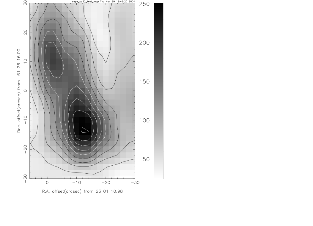
Figure 1: Gray-scale and contour map of the integrated flux in the CO 3 – 2 line of the Cepheus E outflow.

The two outflow lobes are also present in the CO(3 – 2) map (Fig. 1). Note that the two lobes are elongated in a direction mis-aligned from the overall outflow direction. At the brightest points, the line shape shows signs of being optically thick (self absorption and re-emission). High velocity bullets with v${}_{rel}\approx$ 100 km s^-1 are also detected. In the CS(7 – 6) map we found weak emission only near the source position and extremely weak emission at the three brightest knots of the outflow (S1, Na and Nd). Nevertheless, the outflow structure is visible in this line. At the three positions where the CO(4 – 3) line is observed we see the same line structure as for the CO(3 – 2) line: optically thick in the line centre and very fast CO bullets (v${}_{rel}\approx$ 100 km s^-1). The northern positions observed in SiO(8 – 7) show no sign of a line. Only at the two positions in the south very weak emission is detected.

4 Extinction

4.1 Methods

To determine the luminosity and excitation of a deeply-embedded outflow it is necessary to remove the extinction. Extinction reduces observed fluxes from their intrinsic values, especially for those from the shorter wavelength KSPEC data. Hence, in order to test shock models, we first adjust the KSPEC fluxes.

Since the Cep E outflow is embedded in the parental cloud of the source (only the southernmost part is visible at optical wavelengths as HH 377), the extinction is high. Moreover, the extinction may vary not only over the field of the LWS aperture but also through a lobe. That is, the K-band data will be more representative of emission arising from low-excitation regions while ISO and CO data will sample more evenly. Here, however, since we do not have an extinction map and cannot distinguish components of contrasting extinction, we determine the extinction for each KSPEC location and then apply one value per LWS and ISOCAM beam.

Three means are at our disposal to estimate the extinction. First, 1.25 mm continuum emission from cool dust is spatially coincident with the outflow (Lefloch et al., 1996). This can be interpreted as an H column of 6 $\times$ 10²² cm in the lobe locations, corresponding to 3–4 mag of K-band extinction (incorrectly converted by Lefloch et al. (1996)). If half of this emission lies on average in front of the lobe, an extinction of 1.5–2 mag would result. Submillimeter continuum observations yield a mean H₂ column of 3 $\times$ 10²²cm within a 30^′′ radius, consistent with the above result (Chini et al., 2001).

Second, the Q-branch 1–0 lines beyond 2.4$\mu$m arise from the same upper energy levels as the S-branch 1–0 lines within the K-band. Hence, differential extinction between these wavelengths can, in theory, be determined exactly since the number of emitted photons must be proportional to their Einstein coefficients (radiative decay rates). Absolute extinction can then be derived from the differential value provided the properties of the dust are known.

To apply this second method, we adopt a differential extinction of the form $dlog(A_{\lambda})=0.4A_{K}((2.12\mu m)/\lambda)^{1.7}-1.0)$. Using just the 1 – 0 S(1) and 1 – 0 Q(3) lines (both originating from the same upper energy level), we determine K-band extinctions of A${}_{K}\sim$ 2.6 – 3.2 mag for the three KSPEC slit positions. In contrast, the Q(2)/S(0) ratio yields a uniform extinction of just 1.1$\pm$0.1 mag.

The Q-branch lines are, however, greatly effected by transmission and are often inaccurate. One good test for accuracy is to inspect the ratio of the Q(3)/Q(1) lines which should be within the range [0.91,1.12] if filter or transmission distortions are low and if the gas is excited within the range [1500K,3000K] (Smith, 1995). This was not case for the previously derived values in Ladd & Hodapp (1997) and Moro-Martín et al. (2001). Moro-Martín et al. (2001) find values of 0.58 and 0.86 for locations in the two lobes and Ladd & Hodapp (1997) find 0.78 and 0.88. Differential extinction would only exacerbates the inconsistency. Here, we derive Q-branch Q(3)/Q(1) ratios of 1.18, 1.16 and 1.10 for the 3 slits, which are comfortably consistent when some differential extinction is taken into account. Nevertheless, even in this case, extinctions derived from the S(1)/Q(3) and S(0)/Q(2) ratios do not agree.

The third method also employs differential extinction but makes use of a large fraction of the data. We plot the H₂ columns from all the levels across the H and K bands and then determine the extinction range which best correlates the accumulated data. To achieve this result, however, one must apply the normalised Column Density Ratio (CDR) method. Plotting the derived absolute columns of H₂, N_j against the upper energy level, E_j hides the information in the data since columns are spread out over three orders of magnitude while error bars are only 10% on many data points. In the CDR method, the columns are normalised to the 1–0 S(1) flux and divided by the equivalent LTE column of a gas at 2000K (see Froebrich et al. (2002a) and Eislöffel, Smith, & Davis (2000) for details). The results are shown in Fig. 2.

Figure 2: Column density ratios for the near infrared H₂ ro-vibrational data, before applying extinction (top panels) and after adjustment for extinction (lower panels). The slit locations and extinction are indicated on each panel. Upper bounds are displayed as vertical lines. Squares represent 1–0 lines, with lighter squares denoting the less-reliable columns derived from the Q-branch, diamonds indicated 2–1, and triangles indicate CDRs from 3–2 lines.

Fig. 2 confirms that high extinction is present. Extinction is responsible for the distribution of the data points along the edges of a rhombus (top panels), which collapses to a line on applying the extinctions indicated. The four sides of the rhombus consist of (i) the K-band 1–0 S-branch, (ii) 1–0 Q-branch, (iii) 2–1 S-branch and (iv) H-band 1–0 S-branch. We note no evidence for UV excitation and fluorescent emission (as usually identifiable from rotational transitions within the higher vibrational levels). Hence, the CDRs from the 2–1 lines should lie level or below those from the 1–0 lines. However, we also require that the Q-branch lines are not too far below the S-branch lines. In this manner, a good approximation for extinction is reached in each case.

4.2 The intrinsic outflow

The higher K-band extinction in the northern lobe by $\sim$ 0.7 mag implies that this lobe is not intrinsically weaker than the southern lobe in molecular hydrogen emission. The north-south 1–0 S(1) ratio was found by Eislöffel et al. (1996) to be 0.54. This suggests that the outflow may be much more symmetric than appears. Since the northern lobe is redshifted, this is also consistent with the lobe dynamics within a spherical cloud.

The mean density can be estimated on assuming the geometry of the enveloping cloud. Taking a uniform spherical cloud of radius 30^′′, corresponding to 0.11 pc, and an average column to the outflow of $\sim 3\times 10^{22}$ cm^-2, yields a mean (H nuclei) density estimate of $1.3\times 10^{5}cm^{-3}$.

The extinction also implies that the intrinsic H₂ luminosity from the 1–0 S(1) line alone is 0.33 L_⊙, and the total H₂ luminosity will probably lie in the range 3–9 L_⊙, depending on the type and strength of shock waves involved (Smith, 1995). Notably, this total is very close to that estimated for the complete far-infrared cooling by Giannini et al. (2001) of 2.8 L_⊙, which includes CO, H₂O, O and OH emission.

Figure 3: Planar shock models for Cep E South. In addition to the symbols described in Fig 2, the ISOCAM data are represented by stars. (a) A hot C-shock component with 32 km s^-1 provides a fit to the vibrationally-excited columns but does not contribute to the CO rotational lines (other critical parameters are a density of 10⁵ cm^-3, an Alfvén speed 1.5 km s^-1, ion fraction $\chi~{}10^{-6}$, a transverse magnetic field and n(H₂)/(n(H)+2n(H₂)) = 0.3). The maximum temperature is 3160 K. (b) A cool C-shock with speed 11 km s^-1 provides a fit to the rotationally-excited H₂ and CO but does not contribute to the vibrational lines (other critical parameters are as above except n(H₂)/(n(H)+2n(H₂)) = 0.49998). The maximum temperature in the shock is 950 K. Also modelled are abundances of $\epsilon(O)~{}=~{}4~{}10^{-4}$ and $\epsilon(C)~{}=~{}1.5~{}10^{-4}$.

5 H₂ and CO Modelling

To simultaneously model the KSPEC, ISOCAM and LWS CO data, we require a calibration of the KSPEC data set. We employ the integrated 1–0 S(1) K-band fluxes of $1.45\times 10^{-15}~{}Wm^{-2}$ (North) and $2.68\times 10^{-15}~{}Wm^{-2}$ (South) tabulated by Eislöffel et al. (1996) since the associated areas correspond quite closely to the effective apertures of the ISO observations.

We have attempted to apply simple planar J-shock and C-shock models, without success. We have employed an updated shock code described in detail by Smith et al. (2003). The code assumes that a shock is stable and in a steady state, the ion number is a conserved quantity and that the H₂ dissociation rate is given by equilibrium conditions. We take an ortho-para ratio for H₂ of 3. Single J-type shock waves predict high excitation H₂ spectra and C-type shocks predict quite constant excitation across a wide range of upper energy levels.

Multiple shock waves are required, as demonstrated in Fig. 3. Two carefully chosen C-type shocks provide a reasonable fit to the full set of data. The top panel displays both the ISO H₂ data (stars at low T_j) and the KSPEC data. The lower panel displays the CO rotational fluxes. It is not clear, however, how two shocks with almost the same parameters can be found in the three separate locations since the excitation produced in planar shocks is very sensitive to the shock velocity, field strength and ionization fraction.

Next, we fit a single paraboloidal C-type bow shock. C-type and J-type bow shocks are modeled according to a scheme illustrated in Fig. 4. Cylindrical coordinates (z, R, $\phi$) are used, and the magnetic field B, is defined via the density and Alfvén speed. The spectroscopic results presented here are independent of the direction of the observer, $\alpha$. The molecules are completely dissociated at the bow cap provided the bow is moving faster than the appropriate dissociation speed limit. The data provides a large number of constraints. For example, the CO fluxes and excitation determine not only the CO abundance but also the density. The excitation state of the vibrationally excited H₂ also determines the density as well as the shape of the bow. The rotationally-excited H₂ determines the atomic hydrogen fraction.

Figure 4: The geometrical parameters associated with a fast-moving bow shock, as originally employed by Smith and Brand (1990).

The final results are displayed in Fig. 5 for Cep E South and Fig. 6 for Cep E North (location Nd for the KSPEC data). Note that bow configurations are strongly supported by two independent observations. First, the H₂ images display numerous bow-shaped structures in both lobes (e.g. Fig. LABEL:cepe_h2 and Ladd & Hodapp (1997) and, second, many locations within these 1–0 S(1) bows possess double-peaked line profiles, as predicted by bow shock models (Eislöffel, 1997) and numerical simulations Suttner, Smith, Yorke, & Zinnecker (1997).

Figure 5: A C-type bow shock model for Cep E South 1. A C-type bow model with speed 120 km s^-1, a density of 10⁵ cm^-3, an Alfvén speed 1.5 km s^-1, ion fraction $\chi~{}10^{-6}$ and n(H₂)/(n(H)+2n(H₂)) = 0.35, abundances of $\epsilon(O)~{}=~{}3~{}10^{-4}$ and $\epsilon(C)~{}=~{}1.4~{}10^{-4}$ (initially in CO) and a magnetic field aligned with the bow axis. The H₂ model values are displayed for the ground (solid line ), first (dashed) and second (dot-dash) vibrational levels.

Figure 6: A C-type bow shock model for Cep E North (location Nd). The model bow speed is again 120 km s^-1 and critical parameters are as in Fig. 5, except for the initial abundance $\epsilon(CO)=1.2\times 10^{-4}$. Displayed lines on the CDR diagram represent individual vibrational levels (see Fig. 5).

The displayed CBOW model fits are further evidence that these are bow shocks. The ranges of critical parameters determined during the modelling procedure are given in Table 4. Most significant are (i) the density, (ii) the molecular fraction, (iii) the bow shape and (iv) the CO abundance. Less critical parameters to the gas excitation state are (i) the bow speed (the excitation is fixed provided the bow speed exceeds a minimum value), (ii) the Alfvén speed (i.e. the magnetic field), (iii) the ion fraction (a minimum value is necessary for a J-shock to be appropriate) and (iv) the oxygen abundance. The latter parameters influence the location of the molecular emission along the bow surface but, provided the location exists and is not at the apex, the excitation is not strongly affected. Perhaps the most significant result is the atomic hydrogen fraction of 0.1 – 0.4. Additionally, the derived CO abundances at all three locations lie close to $1\times 10^{-4}$.

Table 4: Ranges for the critical parameters which describe the observed shock excitation, as derived by comparing models to both the H₂ and CO data. Location Nd is taken here. The criterion taken as a good fit is a discrepancy of approximately 30% between the majority of data points and the model fluxes.

Model	Bow	Density	Magnetic	Alfvén	Ion	$\epsilon$(C)	$\epsilon$(O)	bow	H2
	speed	105	field	speed	fraction			shape	fraction
	km s-1	cm-3	mG	km s-1	10-7	10-4	10-4
C-type	$>$ 38	0.6–1.2	0.2–1.3	1.0–6.0	4–50	0.6–1.4	1.0–5.0	1.9–2.3	0.32–0.40
J-type	$>$ 17	2.0–5.0	0.3–0.6	1.5–3.7	–	0.3–0.6	1.3–7.0	1.4–1.6	0.14–0.26

Finally, we consider the type of J-type bow shock that could fit the spectroscopic data. Since J-shocks heat the gas impulsively, higher vibrational levels are relatively well populated. Hence, to fit the data, a bow with longer cooled wings than a paraboloid is needed to compensate. After varying the critical parameters, Fig. 7 shows that a bow with shape s = 1.5 where z/L = (1/s)(̇R/L)^s fits the data extremely well.

Figure 7: A J-type bow shock model for Cep E North, position Nd, with shape parameter s = 1.5. A speed of 60 km s^-1, a density of 3 10⁴ cm^-3, an Alfvén speed 2.5 km s^-1, n(H₂)/(n(H)+2n(H₂)) = 0.2, and abundances of $\epsilon(O)~{}=~{}4~{}10^{-4}$ and $\epsilon(C)~{}=~{}5~{}10^{-5}$ (initially in CO) and a magnetic field aligned with the bow axis were taken. The H₂ model values are displayed for the ground (solid line ), first (dashed) and second (dot-dash) vibrational levels.

A major reason that quite blunt shapes are predicted here, in comparison to those derived for Cepheus A, is that lower densities are involved. A lower density is deduced from the relatively low CO fluxes in Cepheus E. The lower density then necessitates a higher fraction of hydrogen atoms to maintain a small divergence from local thermodynamic equilibrium between the populations of the H₂ vibrational levels.

6 Further diagnostics

To distinguish between J and C-type bow models, we examine other signatures. We present the contributions to the cooling, calculated from the two best fitting models to Cep E S1, in Table 5. The luminosities are calculated by assuming a sufficient number of bow shocks to explain the H₂ 1–0 S(1) luminosity. Indeed, a reasonable number of distinct bow shocks are inferred. We find from the above model that a single C-type bow of speed v_bow = 120 km s^-1 and scale size L = 10¹⁵ cm emits 0.016 L_⊙ in the H₂ 1–0 S(1) line. Therefore, 20 such bows in each lobe would suffice to provide the observed luminosity. Note that these bows would appear larger than L in size, with H₂ being thermally dissociated until the normal component of velocity falls below 45 km s^-1. For a paraboloid, it is straightforward to show that this occurs at R = 2.47 L and z = 3.05 L.

A single J-type bow with s = 1.5, v_bow = 60 km s^-1 and scale size L = 10¹⁵ cm emits 0.02 L_⊙. Hence, 16 such bows would be needed to account for the H₂ emission. The apparent bow size is, however, larger. With a dissociation speed limit of 25 km s^-1, we find molecules survive only for bow locations at R $>$ 4.76  L and z $>$ 4.36 L.

Table 5: Contributions to the intrinsic cooling of the flow in Cep E South and the bow shock predictions. The total cooling estimates are extracted from Giannini et al. (2001).

Coolant	Observed	C-Bow	J-Bow
	L⊙	L⊙	L⊙
H2 1 – 0 S(1)	0.33	0.33	0.33
H2 dissociative	–	0.11	0.92
H2 rot+vibrat.	–	6.77	8.32
CO rote	$>$ 0.51	4.76	56.56
CO rote (J $>$ 10)	0.51	1.26	1.38
CO vibe	–	0.01	0.03
H2O	$>$ 0.67	1.53	3.71
H2O (FIR, T$>$800K)	0.67	0.54	1.39
OH	0.17	0.01	0.01
OI 63$\mu$m	$>$ 0.21	1.72	21.36
CI 370$\mu$m	–	0	0.17

The [O I] 63$\mu$m line is potentially a good shock diagnostic. However, the column density of hydrogen nuclei which provides unit optical depth at line centre is just $5\times 10^{20}~{}cm^{-2}$ (Hollenbach & McKee, 1989). This may explain why the model line flux is overpredicted by factors of a few (see Table 5). Given gas columns of $3\times 10^{22}~{}cm^{-2}$, the observed [OI] emission may well not have a shock origin. Furthermore, we also detected the [CII](158 $\mu$m) line in the LWS spectrum. The measured ratio [OI](63 $\mu$m)/[CII](158 $\mu$m) is about 1.3 (1.5) for the north and south lobes, respectively. In shocks, the [CII](158 $\mu$m) line is usually several orders of magnitute fainter than the [OI](63 $\mu$m) Hollenbach & McKee (1989). Hence these lines may have a PDR origin, as already discussed by Moro-Martín et al. (2001). The observed OH luminosity is, according to Giannini et al. (2001), to be treated with caution since it may well be due to continuum pumping.

We conclude from Table 5 that the long wings of the J-type bow produce extremely high fluxes in the lines from the cooler molecular gas. This is inconsistent with all expectations since the total cooling then exceeding the bolometric luminosity of the protostar. Furthermore, in a shock-dissipative momentum-driven outflow, we expect the mechanical power of the flow to be very close to the total cooling. We estimate here the mechanical power through CO J=2–1 observations by first noting that most of the emission is from low-speed CO but most of the kinetic energy lies in the CO moving with radial speeds of 15–25 km s^-1 (Smith, Suttner, & Yorke, 1997) (a result of the very flat line profile found for Cepheus E). Hence, given a blue lobe mass of 0.16 M_⊙ Ladd & Hodapp (1997), we derive a mechanical energy of $\sim 5\times 10^{45}$ erg and a mechanical power $\sim 20~{}L_{\odot}$. Although this estimate is subject to considerable uncertainty, it is consistent with the C-type bow model.

A further diagnostic is provided by the integrated intensity of the CO(3 – 2) emission shown in Fig. 1. The C-bow model predicts a CO(3 – 2)/CO(18 – 17) ratio of 6.0 in contrast to the J-bow model (276) for the southern outflow lobe. The measured ratio is 4 (north) and 2 (south), much nearer to the predictions of the C-type bow model.

The columns in the 0-0 S(3) and 0-0 S(5) appear lower than predicted in the southern lobe. This suggest that the ortho-to-para ratio of H₂ may be under three, the LTE value for high temperatures. This can occur in C-shocks since the gas is gradually heated from a low pre-shock temperature. Therefore, the gas maintains the pre-shock ortho-para ratio. After some heating, however, atomic hydrogen can induce ortho-para conversion (Smith, Davis, & Lioure, 1997).

Note that the distribution of shocks generated by a supersonic turbulent velocity field can produce an excitation that mimics that from a bow shock surface (Eislöffel, Smith, & Davis, 2000). It can be shown that a power law number distribution of shock speeds (with power law index $\alpha=-2s/(s-1)$ where $N\propto v^{-\alpha}$) is required. This also assumes that there is no systematic magnetic field effects although, for bow shocks with moderate Alfvén speeds, we find that the magnetic field direction has an insignificant influence on the excitation.

7 Conclusions

We have analysed the molecular outflow from the Cepheus E-MM source over a broad wavelength range, from the near infrared into the sub-millimeter regime. We combined KSPEC NIR data, ISO mid- and far-infrared spectra and JCMT sub-mm observations. We have concentrated on the properties of the vibrationally and rotationally excited H₂ and CO since sufficient data points exist to permit a simultaneously interpretation in terms of shock models using J- and C-type physics. We investigated planar and curved shocks.

Cepheus E is quite exceptional in its strong radiative power (above 10 L_⊙) and short dynamical age (under 700 yr given an advance speed of over 100 km s^-1). Our main results are as follows:

1. Extinction is most accurately derived by satisfying multiple constraints on the complete NIR data set rather than from specific line ratios. The southern blueshifted lobe has a mean K-band extinction of 1.4 mag and the northern redshifted lobe has extinction in the range 2.1 – 2.4 mag. This is consistent with the extinction being internal to a spherical cloud, with a density of 10⁵ cm^-3 and radius $3\times 10^{17}~{}cm^{-3}$. Remarkably, the extinction-corrected H₂ columns, including the ISO data, demonstrate a state close to local thermodynamic equilibrium.

2. We interpret all the measured H₂ and CO line fluxes simultaneously in terms of shock models. The best fitting models are obtained using shock distributions in the form of bow shocks.

3. C-type physics is strongly favoured mainly because J-type physics predicts extremely strong emission from the low-excitation flanks of a bow, which is not observed. Moreover, for the J-shock model, the outflow power and momentum become implausibly large in comparison to the values found for the protostar and the bipolar outflow, respectively.

4. High resolution H₂ 1 – 0 S(1) imaging has shown that the lobes consist of numerous emission knots of size $1--3\times 10^{15}$ cm (Ladd & Hodapp, 1997). We find that of order 20 such bow shocks, close to paraboloidal in shape, are required by the model to explain the intergrated emission for each lobe.

5. No significant differences in the density or abundances are found between positions. We also find no significant differences in the H₂ excitation when analysing the integrated spectra of a whole outflow lobe or a 6″ $\times$ 6″  pixel-sized part. This is in agreement with Eislöffel et al. (1996) and suggests that the large bows are built up of smaller unresolved bow shocks, generated by flow instabilities.

6. The pre-shock medium is not fully molecular in these models. We have found a mean atomic fraction of $n(H)/(n(H)+2n(H_{2}))=0.4$. With bow speeds of 120 km s^-1, extensive bow apices are predicted within which molecules are completely destroyed. The reformation time is of order 10¹⁷/n_c(H), where n_c(H) is the atomic density in the compressed layers. Hence, a reformation time of $\sim$ 3000 yr may be achieved for n_c(H) = 10⁶ cm^-3.

7. The total mass set into motion by the outflow is low, 0.25 M_⊙ (Ladd & Hodapp, 1997). We estimate a total cloud mass of 5 M_⊙ given a density of 10⁵ cm^-3 and radius 2.2 $\times$ 10¹⁷ cm. With an outflow half-opening angle of $\beta$, a fraction f_c = 1 - cos $\beta$ of the cloud would be disturbed by two lobes. Taking $\beta$ = 20^∘, yields f_c = 0.06, and thus provides a consistent basic model.

High outflow powers have been uncovered from many other Class 0 protostars. Mechanical luminosity exceeds 50% of the bolometric luminosity for all of the Perseus Class 0 sources (Barsony et al, 1998). On the other hand, a few Class 0 protostars such as L1527 and B335 possess relatively weak outflows as measured by total far-infrared luminosities (Giannini et al., 2001) and CO momentum flow rates (Bontemps et al, 1996). In this respect, the Cepheus E outflow could represent a powerful but abrupt evolutionary phase, about to be brought to a halt as underlying jets exit a compact 0.1 pc cloud.

References

- Ayala et al. (2000) Ayala, S., Noriega-Crespo, A., Garnavich, P.M., Curiel, S., Raga, A.C., Böhm, K.-H., Raymond, J. 2000, AJ, 120, 909
- Bachiller (1996) Bachiller, R. 1996, ARA&A, 34, 111
- Barsony et al (1998) Barsony, M., Ward-Thompson, D., André, P., & O’Linger, J. 1998, ApJ, 509, 733
- Black and van Dishoeck (1987) Black, J.H., van Dishoeck, E.F. 1987, ApJ, 322, 412
- Bontemps et al (1996) Bontemps, S., Andre, P., Terebey, S., & Cabrit, S. 1996, A&A, 311, 858
- Cesarsky et al. (1996) Cesarsky, C.J., Abergel, A., Agnèse, P., et al. 1996, A&A, 315, L32
- Chini et al. (2001) Chini, R., Ward-Thompson, D., Kirk, J.M., Nielbock, M., Reipurth, B., Sievers, A., 2001, A&A, 369, 155
- Clegg et al. (1996) Clegg, P.E., Ade, P.A.R., Armand, C., et al. 1996, A&A, 315, L38
- Davis and Smith (1996) Davis, C.J., Smith, M.D. 1996, A&A, 310, 961
- Eislöffel et al. (1996) Eislöffel, J., Smith, M.D., Davis, C.J., Ray, T. 1996, AJ, 112, 2086
- Eislöffel (1997) Eislöffel, J. 1997, IAU Symp. 182: Herbig-Haro Flows and the Birth of Stars, 182, 93
- Eislöffel, Smith, & Davis (2000) Eislöffel, J., Smith, M. D., & Davis, C. J. 2000, A&A, 359, 1147
- Froebrich et al. (2001) Froebrich D., Eislöffel, J., Smith, M.D. 2001, AG Abstr. Ser., 18, 59
- Froebrich et al. (2002a) Froebrich D., Smith, M.D. Eislöffel, J. 2002a, A&A, 385, 239
- Froebrich et al. (2003) Froebrich D., Smith, M.D., Hodapp, K.-W., Eislöffel, J. 2002b, A&A, submitted
- Giannini et al. (2001) Giannini, T., Nisini, B., Lorenzetti, D. 2001, ApJ, 555, 40,
- Hatchell et al. (1999) Hatchell, J., Fuller, G.A., Ladd, E.F. 1999, A&A, 346, 278
- Hollenbach & McKee (1989) Hollenbach, D. & McKee, C.F. 1989, ApJ, 342, 306
- Hodapp et al. (1994) Hodapp, K.-W.; Hora, J. L., Irwin, E., Young, T. 1994, PASP, 106, 87
- Kessler et al. (1996) Kessler, M.F., Steinz, J.A., Anderegg, M.E., et al. 1996, A&A, 315, L27
- Ladd & Hodapp (1997) Ladd, E. F. & Hodapp, K.-W. 1997, ApJ, 474, 749
- Lefloch et al. (1996) Lefloch, B., Eislöffel, J., Lazareff, B. 1996, A&A, 313, L17
- Moro-Martín et al. (2001) Moro-Martín, A., Noriega-Crespo, A., Molinari, S., Testi, L., Chernicharo, J., Sargent, A. 2001, A&A, 555, 146
- Noriega-Crespo and Garnavich (2001) Noriega-Crespo, A., Garnavich, P.M. 2001, AJ, 122, 3317
- Noriega-Crespo et al. (1998) Noriega-Crespo, A., Garnavich, P.M., Molinari, S. 1998, AJ, 116, 1388
- Reipurth & Bally (2001) Reipurth, B. & Bally, J. 2001, ARA&A, 39, 403
- Rousselot et al. (2000) Rousselot, P., Lidman, C., Cuby, J.-G., Moreels, G., Monnet, G. 2000, A&A, 354, 1134
- Smith and Brand (1990) Smith, M.D., Brand, P.W.J.L. 1990, MNRAS, 245, 108
- Smith (1995) Smith, M. D. 1995, A&A, 296, 789
- Smith, Suttner, & Yorke (1997) Smith, M. D., Suttner, G., & Yorke, H. W. 1997, A&A, 323, 223
- Smith et al. (2003) Smith, M. D., Khanzadyan, T., Davis, C.J., 2003, MNRAS, 339, 524
- Smith, Davis, & Lioure (1997) Smith, M. D., Davis, C. J., & Lioure, A. 1997, A&A, 327, 1206
- Suttner, Smith, Yorke, & Zinnecker (1997) Suttner, G., Smith, M. D., Yorke, H. W., & Zinnecker, H. 1997, A&A, 318, 595