A Review of The O–C Method and Period Change

Abstract

The classical O–C curves are discussed in different cases in which various period changes involved. Among them, the analytic O–C curves with frequency, amplitude modulations and with double modes are closely inspected, respectively. As a special, the light-time effect is illustrated. The features of period change noise and period change to metallicity are added at the end.

Keywords:  O–C method–period change

1 Introduction

The O–C diagram is a plot showing the observed times of maximum light(O) minus those calculated according to an adopted ephemeris(C) plotted as a function of time, mostly, the number of elapsed cycles. In the same way, the O–C diagram can also be constructed by the difference between the observed times of maximum radial velocity and the times predicted from an adopted ephemeris. One may find the minima are used instead of maxima for some variables. In particular, the spectroscopic and photometric O–C values are combined to produce a single O–C diagram.

The employment of the O–C diagram almost means normal or regular periodic light curve with a large amplitude is concerned. In other words, the times of maximum light can be determined sufficiently well from the observed light data. One can find ‘O’ by fitting a single sinusoid with an assumed pulsation period to observations. ‘O’ may be derived through local fit to the light curves around individual maxima as well. The latter is very useful in the case of asymmetrical light curves or light curves with changing amplitude such as the cycle-to-cycle or the day-by-day variations.

The Calculated times of maximum light ($C_{n}$) based on an adopted or estimated period ($P_{\rm est}$) and an initial epoch or Time of maximum light ($T_{0}$). Assuming that the observed times of maximum light, ($T_{0},T_{1},T_{2},\cdots,T_{N}$), are determined in different ways depending on different observers, we give O–C series as

$$(O-C)_{n}=T_{n}-(T_{0}+n\,P_{\rm est}),~{}~{}~{}~{}n=0,1,2,\cdots\cdots,N$$ (1)

where n is the cycle number elapsed from the initial epoch at the observed point. Followings refer to different cases of period change in the point of O–C curve.

2 Different O–C Curves

2.1 Period Changing Nothing

At the beginning, we consider the case of period P keeps constant over the time span of observations covered. By assuming that

$$\begin{array}[]{l}P_{\rm est}=P+\delta P,~{}~{}~{}T_{0}^{\rm est}=T_{0}+\delta T_{0}\end{array}$$ (2)

then we can compute O–C as

$$(O-C)_{n}=T_{n}-[T_{0}+\delta T_{0}+n(P+\delta P)]$$ (3)

If $\delta$P=0, namely

$$\begin{array}[]{l}(O-C)_{n}=T_{n}-(T_{0}+\delta T_{0}+nP),~{}~{}~{}\langle(O-C)\rangle=-\delta T_{0}\end{array}$$ (4)

the O–C diagram will consist of points scattered around a horizontal line:

$$(O-C)_{n}=-\delta T_{0}$$ (5)

by assuming $T_{n}-(T_{0}+nP)=O(0.0)$, the same below.
If $\delta T_{0}$=0, that is

$$\begin{array}[]{l}(O-C)_{n}=T_{n}-(T_{0}+nP)-n\,\delta P\end{array}$$ (6)

Clearly, $(O-C){{}_{n}}$ decreases with n increases, the O–C plot will be a straight line:

$$(O-C)_{n}=-n\,\delta P$$ (7)

If $\delta P>0$, that is $P_{\rm est}$ is longer than P, the O–C line will slop downwards; otherwise, $\delta P<0$, slop upwards. A vertical shift of the $(O-C)_{n}$ line relative to $\delta$P=0, $\delta T_{0}$=0 lines in Fig. 1 tells us a shift in the epoch, the change in the phase of variation in other words.

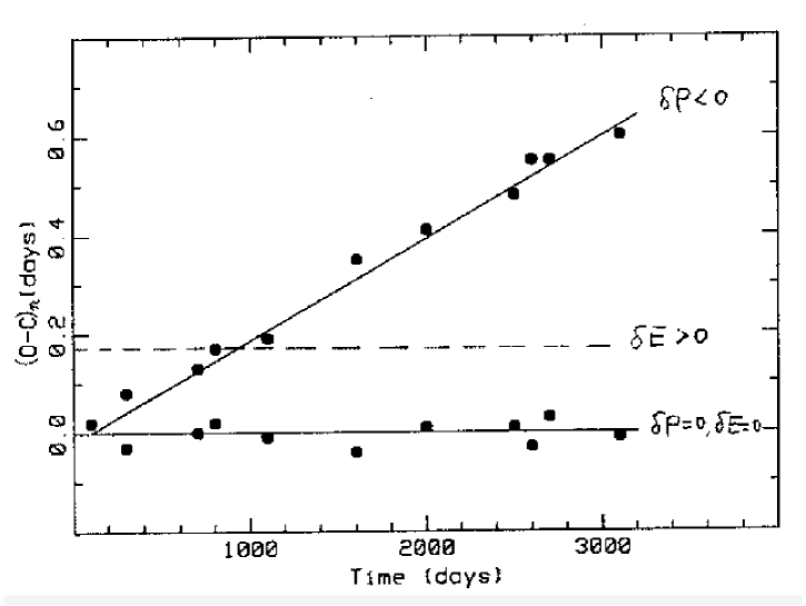
Figure 1: The O–C diagram as a constant period. The slop line, $(O-C)_{n}=n\,\delta P$, refer to the estimated period $P_{\rm est}=P+\delta P$ assuming the intrinsic period P is constant. Here, $\delta$P=O(P)$\ll$ P. Dashed lines, $(O-C)_{n}=-\delta T_{0}$, correspond to the cases in which a correct period value is employed but the initial epoch has an uncertainty of $\delta T_{0}$. Note that the mirror parts are omitted.

2.2 Period Changing with Time

Now, if the period is changing with time, may be increasing or decreasing. Let P(t) stands for a changing period with a slow, constant rate $\beta$ as caused by stellar evolution, we write

$$P(t)=P_{0}+\beta t$$ (8)

The derivative of the equation above gives the rate of period changing $\frac{dP(t)}{dt}=\beta$. The stellar radius or mass changes due to evolutionary effects or mass loss often results in a slowly changing in period. We have

$$\begin{array}[]{l}C_{n}=T_{0}+nP_{0},~{}~{}~{}O_{n}=T_{0}+nP(T_{n})\\ (O-C)_{n}=n[P(T_{n})-P_{0}]=n\beta T_{n},~{}~{}~{}n=0,1,2,\cdots\cdots,N\end{array}$$ (9)

By denoting $\triangle$P as the mean change during one period, when $T_{1}=P,T_{2}=2P,\cdots\cdots,T_{N}=NP$, we obtain

$$P(T_{1})=P_{0}+\triangle P,\cdots\cdots,P(T_{N})=P_{0}+N\triangle P$$ (10)

So during the time span of the observations concerned, the change of the period is

$$(O-C)_{n}=n[P(T_{n})-P_{0}]=\triangle P\,n^{2}$$ (11)

This is a parabola equation (see Fig. 2).

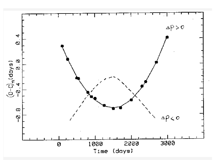
Figure 2: The O–C diagram as the period is changing slowly with time. $(O-C)_{n}=\triangle P\,n^{2}$. The solid curve for $\triangle P>0$, the dashed curve for $\triangle P<0$.

With assumption that

$$C_{n_{0}}=T_{0}+P_{0}\,n_{0},~{}~{}~{}O_{n_{0}}=T_{0}(n_{0})+P_{0}\,n_{0}$$ (12)

we have

$$(O-C)_{n}=(O-C)_{n-n_{0}}+(O-C)_{n_{0}}=\triangle P(n-n_{0})^{2}+(T_{0}(n_{0})-T_{0})$$ (13)

Now the equation demonstrates the information of both the epoch $T_{0}$ and the period change $\triangle$P are included in the O–C diagram. The measured accuracy of period changes increases as $n^{2}$. Hence it is more important to extend the observations for a well-studied variable star.

The predicted evolutionary period changes of variable stars is commonly difficult to be revealed in the O–C diagram because the evolutionary changes may still be too small to be detected after a few tens of years. In that cases, the O–C diagram should be essentially a straight line. In special, in those stars evolving to the red toward the end of their horizontal branch lifetimes, the evolutionary period changes, while still small, ought to be large enough to be detected. In these cases, the O–C diagram should be well represented by a parabolic curve, which should indicate a slow rate of period increase. A few stars might be caught in the interval of core instability, and could show period increases or decreases much larger than $dP/dt$=0.025 days per million years.

Prager (1939) noted that three field RR Lyrae stars’ periods did not change at a constant rate, but were better modeled assuming abrupt period changes. Abruptness, of course, does not accord with a model in which period change results from smooth evolution. Usually, the period changes revealed in the O–C diagram were more abrupt than a perfect parabola would allow. The period changes are small compared to the length of the period itself but because many cycles have passed by, the cumulative effects on the O–C diagram may be large. In some stars, the observations can be well fit by assuming that the period is changing at a constant rate (parabola O–C diagram), but many others follow Prager’s stars seem to have abrupt changes in period. When fit by a parabola, the derived rates of period change are usually in the range of $-$1 to +1 days per million years, or a change of less than 10 seconds during 50–100 years in which the stars have been under observation.

2.3 The Phase-shift Diagram

In addition to the O–C diagram, an analogy, the phase-shift diagram is also applied to interpret period changes in light (e.g. Percy et al. 1980, Breger 1990). Followings show the phase-shift diagram functions exactly the same as the classical O–C diagram. We define quantity $f_{i}$ as below:

$$f_{i}\equiv\frac{t_{i}-t_{0}}{P_{\rm est}}$$ (14)

here $t_{i}$ is the observed times such as times of maximum light of pulsating stars, $t_{0}$ is any arbitrary reference time, $P_{\rm est}$ is an estimated period. The fraction remained of $f_{i}$ constructs the phase $\phi_{i}$, and the integer of $f_{i}$ produces the cycle number N. A plot of the phase against the cycle number is thus called the phase-shift diagram. Under the assumption that the period P is changing uniformly at a rate of $\beta$ described by eq.(8) where $P_{0}$ is the period value at $t_{0}$, t is the time interval passed by from $t_{0}$, hence

$$P_{i}=P_{0}+\beta(t_{i}-t_{0}),~{}~{}~{}~{}i=1,2,3,\cdots\cdots,N$$ (15)

If we take the mean of $P_{0}$ and $P_{i}$, the period at middle point of the two periods is

$$\langle P\rangle=\frac{1}{2}(P_{i}+P_{0})=P_{0}+\frac{1}{2}\beta(t_{i}-t_{0})$$ (16)

we have cycle numbers from $P_{0}$ to $P_{i}$:

$$n=\frac{t_{i}-t_{0}}{\langle P\rangle}=\frac{t_{i}-t_{0}}{P_{0}+\frac{1}{2}\beta(t_{i}-t_{0})},~{}~{}~{}~{}(t_{i}-t_{0})=\frac{n\,P_{0}}{1-\frac{1}{2}\beta n}$$

Such that we find $\phi_{n}$:

$$\phi_{n}=\frac{t_{i}-t_{0}}{P_{\rm est}}-n=\frac{n\,P_{0}}{P_{\rm est}(1-\frac{1}{2}\beta n)}-n$$ (17)

Without loss of generality, $\frac{1}{2}\beta n\ll 1$, we make use of series expansion that

$$\frac{1}{1-\frac{1}{2}\beta n}=\sum_{n=0}^{\infty}(\frac{1}{2}\beta n)^{n}\approx 1+\frac{1}{2}\beta n$$ (18)

therefore,

$$\phi_{n}=\frac{nP_{0}}{P_{\rm est}}(1+\frac{1}{2}\beta n)-n=(P_{0}-P_{\rm est})\frac{n}{P_{est}}+\frac{1}{2P_{\rm est}}P_{0}\beta n^{2}=(P_{0}-P_{\rm est})\frac{n}{P_{\rm est}}+\frac{1}{2}\beta n^{2}$$ (19)

($P_{0}/P_{\rm est}\approx 1,~{}n=1,2,3,\cdots\cdots,N$). The equation presents a parabola about cycle number n. Quantity $\beta$, is generally used to characterize the period change rates of variables. It is the rate of period change determined through fitting a parabola to the O–C diagram, and is normally presented in the unit of days/days or days/year. A unit of days per million years for $\beta$ is chosen by some authors. $\frac{1}{P}\frac{dP}{dt}$ is sometimes presented as the period change rate in unit cycle/year.

3 Analytic O–C Curves

We describe the light brightness of a variable star with a sinusoidal waveform as:

$$L(t)=L_{0}+A\sin(2\pi t/P)$$ (20)

where P is the period of light variation, A is the amplitude of the sinusoidal wave, $L_{0}$ is the zero point. It is well known that the times of maximum light occur at $L^{\prime}(t)=0$, which yields $O_{n}=\{T_{0},T_{1},T_{2},\cdots\cdots,T_{N}\}$. At the same time, $\sin\frac{2\pi C_{n}}{P}\longrightarrow$ 1 and $\cos\frac{2\pi C_{n}}{P}\longrightarrow$ 0, at the times of maximum light. The period changes in the light curves are discussed in several different sources below.

3.1 Frequency Modulation

For frequency or period modulation, theoretical light curve is defined by

$$L_{\rm f}(t)=L_{0}+A\sin(2\pi t/P(t))$$ (21)

$L_{\rm f}^{\prime}(t)$=0 produces $O_{n}$ as

$$O_{n}=\frac{P(t)}{4}(2n+1),~{}~{}n=0,1,2,\cdots\cdots,N$$ (22)

$C_{n}$ are naturally derived from $L(t)=L_{0}+A\sin(2\pi t/P)$, so

$$(O-C)_{n}=\frac{1}{4}(2n+1)(P(t)-P),~{}~{}~{}~{}~{}~{}n=0,1,2,\cdots\cdots,N$$ (23)

Recalling eq.(8): $P(t)=P+\beta t=P+\beta Pn$ which means $\beta$ is the period change over one cycle, thus

$$(O-C)_{n}=\frac{1}{2}\beta Pn^{2}+\frac{1}{4}\beta Pn$$ (24)

this is a parabola with respect to cycle number n.

3.2 Amplitude Modulation

The change in period caused by the variability of amplitude called amplitude modulation is described as:

$$L_{\rm a}(t)=L_{0}+A(t)\sin(2\pi t/P),~{}~{}~{}A(t)\equiv a\sin(2\pi t/P_{\rm A})$$ (25)

A(t) refers to a sinusoidal amplitude modulation which causes a secondary period $P_{\rm A}$ in the light curve. The calculus of $L_{\rm a}$(t), $L_{\rm a}^{\prime}(t)$, gives observed times of maximum light $O_{n}$:

$$\frac{1}{P_{\rm A}}\cos\frac{2\pi O_{n}}{P_{\rm A}}\sin\frac{2\pi O_{n}}{P}+\frac{1}{P}\sin\frac{2\pi O_{n}}{P_{\rm A}}\cos\frac{2\pi O_{n}}{P}=0$$ (26)

By making use of the replacement of $O_{n}=(O-C)_{n}+C_{n}$ just for the triangle functions involving P and expanding them. Without loss of generality we presume

$$(O-C)_{n}\ll P;~{}~{}~{}~{}\sin\frac{2\pi(O-C)_{n}}{P}\approx\frac{2\pi(O-C)_{n}}{P}$$ (27)

and with the help of the features mentioned in the beginning of this section: $\sin\frac{2\pi C_{n}}{P}\longrightarrow 1$, we find

$$\frac{1}{P_{\rm A}}\cos\frac{2\pi O_{n}}{P_{\rm A}}(\frac{2\pi(O-C)_{n}}{P}\cos\frac{2\pi C_{n}}{P}+\cos\frac{2\pi(O-C)_{n}}{P})+$$

$$\frac{1}{P}\sin\frac{2\pi O_{n}}{P_{\rm A}}(\cos\frac{2\pi(O-C)_{n}}{P}\cos\frac{2\pi C_{n}}{P}-\frac{2\pi(O-C)_{n}}{P})=0$$ (28)

Expanding similarly now the two functions including $P_{\rm A}$, and recalling that $\cos\frac{2\pi C_{n}}{P}\longrightarrow$ 0, $\cos\frac{2\pi(O-C)_{n}}{P}\longrightarrow$ 1, $L_{\rm a}^{\prime}(t)=0$ becomes

$$\frac{1}{P_{\rm A}}\cos\frac{2\pi(O-C)_{n}}{P_{\rm A}}\cos\frac{2\pi C_{n}}{P_{\rm A}}-\frac{1}{P_{\rm A}}\frac{2\pi(O-C)_{n}}{P_{\rm A}}-$$

$$\frac{1}{P}\frac{[2\pi(O-C)_{n}]^{2}}{PP_{\rm A}}\cos\frac{2\pi C_{n}}{P_{\rm A}}-\frac{1}{P}\frac{2\pi(O-C)_{n}}{P}\cos\frac{2\pi(O-C)_{n}}{P_{\rm A}}=0$$

Note that the coefficient of the third term of the equation above is infinitely small at higher order of $\frac{(O-C)_{n}}{P}$ which is set to almost zero as our original consideration. This yields

$$2\pi(O-C)_{n}(-\frac{1}{P_{\rm A}^{2}}-\frac{1}{P^{2}}\cos\frac{2\pi(O-C)_{n}}{P_{\rm A}})+\frac{1}{P_{\rm A}}\cos\frac{2\pi(O-C)_{n}}{P_{\rm A}}\cos\frac{2\pi C_{n}}{P_{\rm A}}=0$$ (29)

When $P_{\rm A}$ is so large enough that $\frac{(O-C)_{n}}{P_{\rm A}}\ll$ 1, we can make following simplifications:

$$\cos\frac{2\pi(O-C)_{n}}{P_{\rm A}}\approx 1-\frac{2\pi(O-C)_{n}}{P_{\rm A}},~{}~{}~{}\frac{[2\pi(O-C)_{n}]^{2}}{P_{\rm A}}\approx 0$$ (30)

Consequently, we get

$$(O-C)_{n}=\frac{P_{\rm A}}{2\pi}\frac{\cos\frac{2\pi C_{n}}{P_{\rm A}}}{1+(\frac{P_{\rm A}}{P})^{2}+\cos\frac{2\pi C_{n}}{P_{\rm A}}}$$ (31)

This relation shows the shape of O–C is predominated by the modulation period $P_{\rm A}$. If $P_{\rm A}\approx P$, like cycle-to-cycle modulation,

$$(O-C)_{n}\approx\frac{P_{\rm A}}{2\pi}$$

that indicates a shift of $P_{\rm A}/2\pi$ with respect to the zero line showing constant periodic light. In the case of great difference between $P_{\rm A}$ and P, if $P_{\rm A}\gg P$, the long-term amplitude modulation, stimulation shows only a tiny scatter around the zero of the O–C, while $P_{\rm A}\ll P$, the high frequency amplitude modulation, the feature of the O–C is of the behaviour of periodic amplitude variation, we have after neglecting the term including P in eq.(29),

$$(O-C)_{n}=\frac{P_{\rm A}}{2\pi}\cos\frac{2\pi(O-C)_{n}}{P_{\rm A}}\cos\frac{2\pi C_{n}}{P_{\rm A}}$$ (32)

A sinusoidal light curve with an amplitude modulation may have a significant variation in O–C, while a saw-tooth light curve with the same amplitude modulation will show an absolutely flat O–C.

3.3 Double Mode Case

As for double-mode variables with small amplitudes, we choose:

$$L_{\rm d}(t)=L_{0}+Asin\frac{2\pi t}{P_{1}}+Bsin(\frac{2\pi t}{P_{2}}+\phi)$$

Let $L_{\rm d}^{\prime}(t)$=0 for finding $O_{n}$ and so $(O-C)_{n}$. Replacing $O_{n}$ with $(O_{n}-C_{n})+C_{n}=(O-C)_{n}+C_{n}$. With assumption of $(O-C)_{n}\ll P_{1}$, so $\cos\frac{2\pi(O-C)_{n}}{P_{1}}\longrightarrow 1$, $\sin\frac{2\pi(O-C)_{n}}{P_{1}}\approx\frac{2\pi(O-C)_{n}}{P_{1}}$ and $\sin\frac{2\pi(O-C)_{n}}{P_{2}}\approx\frac{2\pi(O-C)_{n}}{P_{2}}$, and recall that we want to find $P_{2}$ in the O–C diagram. Therefore, the expanding of $L_{d}^{\prime}(t)$=0 is equivalent to

$$\frac{P_{2}}{P_{1}}\cdot\frac{A}{B}\cdot\frac{2\pi(O-C)_{n}}{P_{1}}\sin\frac{2\pi C_{n}}{P_{1}}+\frac{2\pi(O-C)_{n}}{P_{2}}\sin(\frac{2\pi C_{n}}{P_{2}}+\phi)=\frac{P_{2}}{P_{1}}\cdot\frac{A}{B}\cdot\cos\frac{2\pi C_{n}}{P_{1}}+\cos(\frac{2\pi C_{n}}{P_{2}}+\phi)$$

thus we have $(O-C)_{n}$ like

$$(O-C)_{n}=\frac{1}{2\pi}\frac{\frac{P_{2}}{P_{1}}\frac{A}{B}\cos\frac{2\pi C_{n}}{P_{1}}+\cos(\frac{2\pi C_{n}}{P_{2}}+\phi)}{\frac{P_{2}}{P_{1}^{2}}\frac{A}{B}\sin\frac{2\pi C_{n}}{P_{1}}+\frac{1}{P_{2}}\sin(\frac{2\pi C_{n}}{P_{2}}+\phi)}$$ (33)

At the times of maximum light, we know $\cos\frac{2\pi C_{n}}{P_{1}}\longrightarrow 0,~{}\sin\frac{2\pi C_{n}}{P_{1}}\longrightarrow 1.$  Finally, we get

$$(O-C)_{n}=\frac{P_{2}}{2\pi}\frac{\cos(\frac{2\pi C_{n}}{P_{2}}+\phi)}{(\frac{P_{2}}{P_{1}})^{2}\frac{A}{B}+\sin(\frac{2\pi C_{n}}{P_{2}}+\phi)}$$ (34)

For the two different periods, $P_{2}/P_{1}\sim 0.78$ is the normal case for the large-amplitude $\delta$ Sct stars. Taking a common amplitude ratio value of 0.30 and a second period of 0.03 d we may simplify eq.(34) to be

$$(O-C)_{n}\sim\frac{0.005\cos(\frac{2\pi C_{n}}{P_{2}}+\phi)}{0.2+\sin(\frac{2\pi C_{n}}{P_{2}}+\phi)}$$

Beating phenomenon can also be involved in the feature of the O–C curve when the two periods are closely spaced with near amplitudes. Furthermore, the effects of the beating will be particularly obvious in the times of maximum light, giving a large O–C amplitude. An interference of two oscillations with the same amplitude A for a suspect $\beta$ Cep star, 53 Psc (Wolf 1987), leads to the amplitude modulation of the form:

$$A_{\rm b}=A\sqrt{2(1+cos\frac{2\pi t}{P_{\rm b}})},~{}~{}~{}\frac{1}{P_{\rm b}}=\frac{1}{P_{2}}-\frac{1}{P_{1}}$$ (35)

here $P_{b}$ is the beat period. Based on this equation, the time required for the amplitude to reach a certain value $A_{obs}$, counted from the epoch of $A_{\rm b}$=0, can be derived as

$$\triangle t\approx\frac{P_{\rm b}A_{\rm b}}{2\pi A}$$ (36)

One more example is the light-time effect in a binary system if $P_{2}\gg P_{1}$, from which the O–C curve may be interpreted,

$$(O-C)_{n}=\frac{P_{1}^{2}}{2\pi P_{2}}\cdot\frac{B}{A}\cos(\frac{2\pi C_{n}}{P_{2}}+\phi)$$ (37)

The information revealed by the O–C diagram depends on both ‘O’ constructed from maxima (often used for pulsating stars) or minima (as in binary) and the methods used to derive the ‘O’ from the data. Usually four ways to find ‘O’, we take

• the time of maximum brightness for each single observation;

• the time of maximum brightness in a smoothed light curve;

• the phase of the maximum of a representative mean light curve fitted to all or a portion of the observations over that cycle;

• the time of maximum derived from an exact solution for a Fourier series which has been fitted to the data.

4 The Light–Time Effect of A Binary

If a pulsating star is a member of a binary system, an independent estimate of the mass from stellar pulsation theory can be given. This is the intention of the detection of the light-time effect (LTE) of a pulsating star.

4.1 Examples of Three $\beta$ Cep Stars

Pigulski has throughly investigated the nature of the period changes of three large-amplitude $\beta$ Cephei-type stars: $\beta$ Cephei itself (the prototype of this class), $\sigma$ Scorpii and BW Vulpeculae in terms of the combined O–C diagram constructed from both the light and radial velocity data. It was shown that the observed period changes were caused by the superposition of a constant-rate period change originated from normal stellar evolution and of the light-time effect in a binary system.

Pigulski and Boratyn (1992) proposed that the observed changes of $\beta$ Cephei (=HR 8238=HD 205021, V=3.23, B1 IV) can be understood in terms of orbital motion of the variable in a binary system, in which the secondary is the less massive companion resolved by speckle interferometry. In fact, the companion in the system of $\beta$ Cep was found in the speckle interferometric way by Gezari et al. (1972). By assuming that the orbital motion is the unique cause of the observed variation of the pulsation period,

$$P_{\rm puls}=P_{0}(1+\frac{V_{\rm rad}}{c})$$ (38)

$V_{\rm rad}$ is fully described by six elements of the spectroscopic orbit: $\gamma$, radial velocity of the system’s barycentre; $P_{\rm orb}$, orbital period; $K_{1}$, semi-amplitude of the radial velocity curve, due to orbital motion of the variable; $e$, eccentricity of the orbit; $\omega$, longitude of periastron; $T_{0}$, the time of periastron passage. The analyses of a single O–C diagram constructed in terms of both the photometric and radial velocity times of maximum offered by Pigulski and Boratyn (1992) show that the apparent changes of the pulsation period of $\beta$ Cep can be explained by the light-time effect, induced by the orbital motion of the variable around the barycentre of the variable-speckle companion system.

$\sigma$ Scorpii (=HR 6084=HD 147165, B1 III) is a quadruple system. Its light variability can be described as a superposition of four periodic terms( Jerzykiewicz & Sterken 1984), of which the main pulsation period $P_{2}$= $0^{d}$.24684 and $P_{1}$=0^d.23967 are also observed in radial velocity. The combined O–C diagram using the times of maximum radial velocity and light displays both an increase and a decrease of the main pulsation period. The period changes seen in the O–C curves can be explained neither by an evolutionary effect nor by LTE alone.

$$(O-C)_{\rm LT}=(O-C)+0^{d}.000015\,E-1^{d}.29\times 10^{-10}\,E^{2}$$ (39)

In fact, both effects contributed to the observed changes of the main pulsation period of $\sigma$ Sco. And LTE is caused by the speckle tertiary. Due to the observations do not cover the whole orbital period of the tertiary, the $(O-C)_{\rm LT}$ diagram cannot help to give a more accurate value of the orbital period than that provided by Evans et al. (1986), is of the order of 100–350 yr. In this sense, the spectroscopic elements are unavailable from the $(O-C)_{\rm LT}$ diagram. But it is sure that the changes seen in the $(O-C)_{\rm LT}$ diagram can be fully explained by the orbital motion (Pigulski 1992).

BW Vulpeculae (=HR 8007=HD , V=6.55, B2 III) is a monoperiodic large-amplitude $\beta$ Cep star. Odell (1984) and Jiang Shi-Yang (1985) showed that the parabolic fit to the O–C diagram of BW Vul yields periodic residuals. Both authors attributed these residuals to LTE induced by the motion of the star in a binary system with an orbital period of about 25 yr. Pigulski (1993) showed that the combined effect of the increase of period with a rate of +2.34 s/cen and LTE in a binary system ($P_{\rm orb}$=33.5$\pm$0.4 yr) fully accounts for the observed changes of the pulsation period of BW Vul. The light-time effect in the $(O-C)_{\rm LT}$ diagram is, for the time being, the only observational evidence for the presence of a companion to BW Vul (see Fig. 3). For BW Vul, the times of minimum light and of minimum radial velocity were used in the determination of period changes. One ephemeris of minimum radial velocity was adopted so as to produce a single O–C diagram.

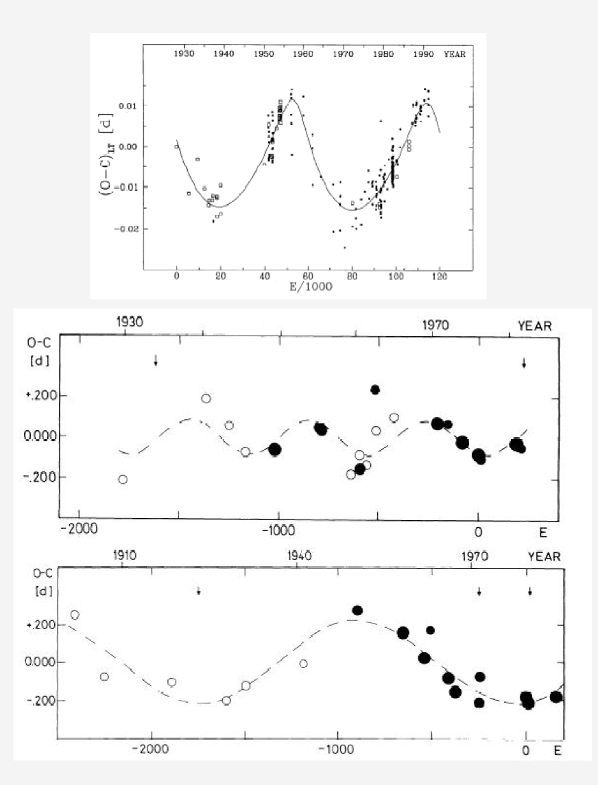
Figure 3: The O–C diagrams showing the light-time effect. Upper panel: $(O-C)_{\rm LT}$ for the $\beta$ Cep star BW Vul, the changes seen in this figure are interpreted as the light-time effect only. Continuous line represents the best fit, from which spectroscopic elements of the orbit are determined. After Pigulski (1993). Lower panels: sinusoidal variations in the O–C curves of the Cepheids FN Aql and RX Aur. Open circles denote the residuals obtained from photographic observations; photoelectric measurements are marked with dots. The size of these symbols refers to the weight assigned. Courtesy of Szabados (1988).

All periodic variables with stable periods such as pulsating stars, eclipsing binaries and pulsars offer the possibility of detecting unseen companion(s) by means of the light-time effect. A pulsating star is a promising candidate for the detection of LTE provided that it belongs to a binary or multiple system. A simplest case is the LTE in a double system with a circular orbit. In the O–C diagram, the changes of the period P of a signal emitted by the visible component (pulsating primary) due to LTE will have the form of a sine curve with semi-amplitude equal to $P_{\rm orb}\,K_{1}/2\pi c$, where $2K_{1}$ is the range of the primary’s radial velocity curve, $P_{\rm orb}$ is the orbital period. The amplitude of LTE depends proportionally on $P_{\rm orb}$ and $K_{1}$ and is equal to the time which light needs for passing the projected orbit. For a given orbital period, short-period variables are more suitable for the study of LTE than the long-period ones because the visibility of LTE depends on the $P_{\rm orb}/P$ ratio. Pigulski (1995) listed 10 objects including eclipsing binaries for which period changes attributable to LTE are observed.

4.2 The Binary Model of The $\delta$ Sct Star CY Aqr

The possibility that CY Aqr is a spectroscopic binary (see Fig. 4) immediately leads to the hope that a mass can be determined. In Figure 5 we show the relationship between the masses of the two companions for assumed values of the orbital inclination. The curve for $i=90^{\circ}$ sets a lower limit to $m_{2}$ at each $m_{1}$. Recent results given by McNamara et al.(1996) indicate: $m_{1}$=1.06 M_⊙, $M_{v}$=2.5. For this mass value of the primary star $m_{2}$ rounds 0.15 M_⊙. The companion must be fainter than CY Aqr by about 8.8 mag. We stress that, the binary model seems to us to be the most plausible interpretation of the variable times of maximum light. It remains only a reasonable hypothesis until new confirming data are available. The simplest and most easily accomplished test is to examine the radial velocity of CY Aqr with a 1.4 km s^-1 amplitude predicted by the model.

Figure 4: The O-C diagram of CY Aqr (cycles) and the curve fitted using both a parabolic curve and a trigonometric function (solid line).

Figure 5: Solutions to the mass function for various choices of $\sin i$ .

5 Period Change Noise

Some stars appear to be unchanged in period over the time span of observations; others have undergone multiple changes in period. Some stars have exhibited both an increase and a decrease in period, as can be seen in the O–C diagram of RR Gem in Fig. 6. Stellar evolution is not expected as we know to act so quickly as to cause period changes in both directions in so short a span. Moreover, the sizes of the observed period changes are often much larger than expected from theory. We call this difference as “period change noise”. In this regard, it is not unquestionable to attribute the period changes observed in any individual star to evolution alone.

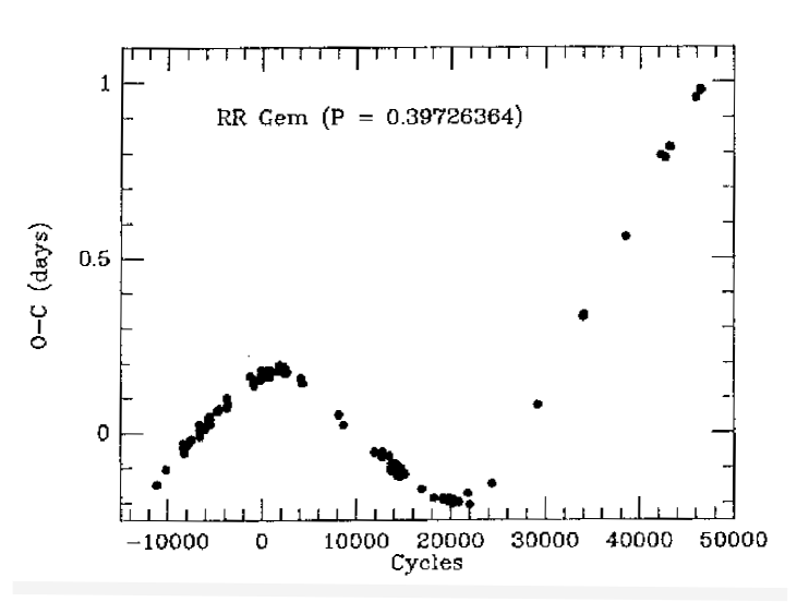
Figure 6: The O–C diagram for the times of maximum light of RR Gem, after Smith (1995).

The period change noise is a result of random mixing events associated with the semiconvective zone of the stellar core (Sweigart and Renzini 1979). The changes in the internal structure of a variable star arise in two ways: through the gradual change in core composition caused by nuclear burning, but also through a composition redistribution in the deep interior caused by convective overshooting and the formation of a semiconvective zone. Whereas this composition redistribution is assumed in standard calculations to proceed smoothly on the same timescales as nuclear burning. The nuclear reaction and convection need not be perfectly coupled at every instant of time. For an actual star, the composition redistribution is a discontinuous process. There might then be many mixing events, each slightly altering the internal of the star, and each leading to a change in period. Furthermore, different types of mixing events can account for both period increasing and decreasing. The observed timescales of period changes are in at least rough agreement with the mixing event hypothesis. Nuclear burning would be expected to produce a slow rate of period change which would be essentially  unvarying over the span of a century. The mixing events, on the other hand, if they took place quickly would produce period changes which would seem abrupt; to the contrary, on a longer timescale they might produce period changes which, for one hundred years, would seem constant in rate. Of course, over a sufficiently long period of time, the period changes due to nuclear burning and discrete mixing events at the semiconvective zone must average to the value predicted by those evolutionary calculations which assume that the composition redistribution takes place  smoothly.

As another  origin for the period change noise, proposed by Stothers (1980), which invoking hydromagnetic effects (such as for RR Lyrae stars). It is a common phenomenon involving stellar magnetism.

Third, Dearborn et al. (1990) suggested that exotic particles, such as weakly interacting massive particles (WIMPS), might produce changes in the pulsation periods (say of RR Lyrae stars). The existence of these particles has been postulated to explain the apparent existence of large amounts of dark matter in galaxies. These particles might become trapped within stars, where they can provide a new mechanism of energy transfer. In the case of horizontal branch stars, WIMPS might cause thermal pulses to occur on the Kelvin-Helmholtz timescale for the stellar core. These thermal pulses would produce period changes. The timescale calculated for these changes, however, on the order of $10^{6}$ yr, is too long to explain the shorter term period noise.

Fourth, the light travel time effect because of orbital motion in a binary stars system may be another possible source for apparent period changes as in RR Lyrae variables identified by Coutts (1971), and in $\beta$ Cephei stars inspected by Pigulski & Boratyn (1992) and Pigulski (1992, 1993). The motion of a star in a binary system could introduce a long term periodic oscillation in the O–C diagram for the time of maximum light, as the star alternately approaches and  recedes from us. It is difficult, however, to build a case for the binary nature of any  variables  from O–C data alone. The examples are comparatively few. Saha and White (1990) have argued on the basis of O–C data and radial velocity observations that TU UMa, a RR Lyrae stars, may be a binary; Barnes III and Moffett(1975) and Moffett et al. (1987, 1988) evidenced the duplicity of SZ Lyncis, a dwarf Cepheid; others as BS Aqr (Fu Jiang-Ning et al. 1997), CY Aqr(Zhou Ai-Ying & Fu Jiang-Ning 1998), BE Lyn (Kiss & Szatmary 1995, Liu et al. 1994, Tang et al. 1992, Liu et al. 1991), BW Vul (Pigulski 1993) and so on (we refer the reader to examples preceded by Pigulski 1993, 1995). However, does the binary hypothesis by itself provide an adequate explanation for the period change behavior?

Finally, mass loss might alter the theoretical period changes. For stars on the horizontal branch lost their masses when they were in the instability strip, that is, when they were RR Lyrae stars. But, the predicted rates of period changes were not significantly changed for mass loss rates as high as $10^{-9}$M_⊙/yr.

6 Period Change to Metallicity

As a variable star evolves through the H–R diagram, crossing its various stages of evolution, the metal abundance or chemical composition changes as well as its period does. In other words, at each given effective temperature periods vary with metallicity. Thus it is natural there is some correlation between the two observable quantities. In real, the period change depends on the change of chemical abundance. We write the relationship of the period change with respect to metallicity, P—[Fe/H], as

$$\frac{dP}{dt}=\frac{dP}{dt}([Fe/H],P)$$

The spectral type determined from the hydrogen Balmer lines (termed Sp(H)) was often later than the spectral type determined from the prominent Ca II K line at 3933Å(termed Sp(K)), which investigated by Preston (1959) under a low resolution spectroscopic survey of RR Lyrae stars in the solar vicinity. On the basis of the difference, Preston then proposed $\triangle S$ index as an indicator of metal abundance (hereafter the $\triangle$S method):

$$\triangle S=10[Sp(H)-Sp(K)]$$ (40)

which was later on confirmed by the analyses of high resolution spectra of RR Lyrae stars (Preston 1961; Butler 1975) and of model stellar spectra (Manduca 1981). Butler(1975) derived

$$[Fe/H]=-0.23-0.16\triangle S$$ (41)

Blanco(1992)  further improved above as

$$[Fe/H]=-(0.34\pm 0.02)-(0.18\pm 0.05)\triangle S$$ (42)

Based on the globular cluster metallicity scale (adopted by Zinn & West 1984, and Zinn 1985), Suntzeff et al. (1991) got following calibration,

$$[Fe/H]=-0.408-0.158\triangle S$$ (43)

is about 0.2 dex more metal-poor than Butler’s scale. In the case of RRab stars, lower $\triangle$S (high metallicity), smaller period changes; higher $\triangle$S (low metallicity), bigger period changes. Iron abundance [Fe/H] is  inferred from the strength of the calcium H-line. Certainly, such a calibration does not require that [Fe/H] = [Ca/H]. Thus, it does require that there exist a one-to-one correlation between iron and  calcium abundances. In fact, [Ca/H] appears to be slightly high compared to [Fe/H] for metal-poor stars in general. Manduca (1981) provided an approximate relation as

$$[Ca/H]=0.8[Fe/H]$$ (44)

for theoretical calibration of the $\triangle$S index.

In addition to the method, other metallicity indicators have also been developed. The photometric indices among which are Sturch’s(1966) broadband ultraviolet blanketing index $\delta$(U-B), the photometric k-line index $(k-b)_{2}$ (Jones 1971, 1973), the Strömgren $m_{1}$ index (Epstein 1969, Epstein and Epstein 1973), and the Walraven system $\delta$[B-L] index (Lub 1977, 1979). In brief, metallicity can be estimated from $\triangle S$(Preston), $(k-b)_{2}$(Jones), $\triangle(B-L)$ (Walraven), $\delta(U-B)$ (Sturch) and $\delta m_{1}$ (Strömgren photometry). For the range 0$\leq\triangle$ S$\leq$12, we have relationships below among the approaches:

$$\begin{array}[]{l}\triangle S=-84\delta(U-B)+14\\ \triangle S=-44(k-b)_{2}+10\\ \triangle S=-99(m_{1})_{0}+16\end{array}$$ (45)

(Butler 1975) and

$$\triangle S=11.9-194\triangle[B-L]+815(\triangle[B-L])^{2}$$ (46)

(Blanco 1992). If metallicity did not change over the pulsation cycle of the star, these indices would remain constant. Rodríguez et al.(1990) failed a test of this internal consistency in the fact of SX Phe and the large amplitude $\delta$ Sct stars. Instead, they concluded that the $m_{1}$ index variation is larger when the metal abundance is smaller.

7 Ending Remarks

The O–C diagram provides us the accurate period and maximum epoch of a variable star, a detector of its period and phase changes, and the information about the spectroscopic orbital elements if it is a binary. Plus, the O–C data provide constraints on stellar evolution theory. For binary systems, O–C analyses of eclipses can reveal very gradual changes due to tidal interactions, or even to gravitational radiation.

The information of period changes is also presented as a phase diagram instead of a classical O–C diagram. Various shapes of the O–C curves correspond to following different cases:

1. The O–C diagram for a star without measurable changes in period is a straight line.

2. If the period of the star is constant, and if the correct period has been adopted, points on the O–C diagram will scatter around a straight horizontal line (see Fig. 1).

3. If the period of the star is constant, but the adopted period is too long or too short, the straight line will slop up or down (see Fig. 1).

4. If the period of the star is changing at a slow, constant rate (i.e. $P(t)=P_{0}+\beta t$ where $\beta$ is small), then a good approximation of the O–C diagram can be represented by a parabola (see Fig. 2).

5. If the period change is caused by the light-time effect in a binary system, the light curve appears to be sinusoidal (see Fig. 3).

6. Broken lines—abrupt or jump changes of period (see Fig. 6).

In order to interpret an O–C diagram correctly, it is necessary to know a number of cycles have elapsed between two observed maxima or since an initial epoch. The determination of elapsed cycles from an epoch is not always easy and reliable especially while the period of the star has been changing significantly.

All common period-finding techniques assume that the periods are constant over the time span of the observations and that the phases are stable. However, these conditions are not always met by variables. Therefore, the O–C method is, in fact, one of the necessities of period analysis. A short review on the O–C method we refer to Willson (1986), a detailed theoretical study may be also referred to the paper series published in MNRAS (Koen &Lombard 1993, 1995; Lombard & Koen 1993; Koen 1996). Koen and Lombard had paid scrupulous attention to the O–C methodology. They pointed out that the problem suffered from within the O–C method that the series of intervals among times is non-stationary so that the applications of this technique may lead to spurious conclusions. As well, they modelled the period changes in variable stars on a quantitative basis, especially supplied tests for the presence of intrinsic scatter in the periods of the long-period pulsating stars.

Acknowledgements
This work was supported by the National Natural Science Foundation of China.

References

Barnes III T. G. and Moffett T. J., 1975, AJ, 80, 48
Blanco V., 1992, AJ, 104, 734
Breger M., 1990, in Confrontation Between Stellar Pulsation and Evolution, eds. C. Cacciari and G. Clementini, ASP Conf. Ser., Vol.11, p.263
Butler D., 1975, ApJ, 200, 68
Coutts C. M., 1971, in New Directions and New Frontiers in Variable Star Research, veroff. der Remeis-Sternwarte Bamberg, IX, Nr. 100, 238
Dearborn D., Raffelt G., Salat P., Silk J., and Bouquet A., 1990, ApJ, 354, 568
Epstein I., 1969, AJ, 74, 1131
Epstein I. and Epstein A. E. A., 1973, AJ, 78, 83
Evans D. S., Mcwilliam A., Sandmann W. H., Frueh M., 1986, AJ, 92, 1210
Fu Jiang-Ning, Jiang Shi-Yang, Gu Sheng-Hong, Qiu Yu-Lei, 1997, IBVS No.4518
Gezari D. Y., Labeyrie A., Stachnik R. V., 1972, ApJ, 173, L1
Jerzykiewicz M. and Sterken C., 1984, MNRAS, 211, 297
Jiang Shi-Yang, 1985, Acta Astrophys. Sinica, 5, 192
Jones D. H. P., 1971, MNRAS, 154, 79
Jones D. H. P., 1973, ApJS, 25, 487
Kiss L.I. and Szatmary K., 1995, IBVS No.4166
Koen C., 1996, MNRAS, 283, 471(IV)
Koen C. and Lombard F., 1993, MNRAS, 263, 287(I)
Koen C. and Lombard F., 1995, MNRAS, 274, 821(III)
Liu Yan-Ying, Jiang Shi-Yang, Cao Ming, 1991, IBVS No.3606
Liu Zong-Li and Jiang Shi-Yang, 1994, IBVS No. 4077
Lombard F. and Koen C., 1993, MNRAS, 263, 309(II)
Lub J., 1977, A&AS, 29, 345
Lub J., 1979, AJ, 84, 383
Manduca A., 1981, ApJ, 245, 248
McNamara, D. H., Powell, J. M., and Joner, M. D. 1996, PASP, 108, 1098
Moffett T.J., Barnes III T.G., Fekel F.C., et al., 1987, Bull. Am. Astron. Soc., 19, 1085
Moffett T.J., Barnes III T.G., Fekel F.C., et al., 1988, AJ, 95, 1534
Odell A. P., 1984, PASP, 96, 657
Percy, J. R., Mattews, J. M., and Wade, J. D. 1980, A&A, 82, 172
Pigulski A., 1992, A&A, 261, 203
Pigulski A., 1993, A&A, 274, 269
Pigulski A. and Boratyn D. A., 1992, A&A, 253, 178
Pigulski A., 1995, in Astronomical and Astrophysical Objectives of Sub-Milliarcsecond Optical Astronomy. eds. E. H$\o$g and P. K. Seidelmann, IAU Symp., Vol.166, p.205
Prager R., 1939, Harv. Bull., No.911, 1
Preston G. W., 1959, ApJ, 130, 507
Preston G. W., 1961, ApJ, 134, 633
Rodríguez E., López de Coca P., Rolland A., Garrido R., 1990 , Rev. Mexican Astron Astrof., 20, 37
Saha A. and White R. E., 1990, PASP, 102, 148(erratum: 102, 495)
Smith H. A., 1995, RR Lyrae Stars, Cambridge University Press, Cambridge
Stothers R., 1980, PASP, 92, 475
Sturch C., 1966, ApJ, 143, 774
Suntzeff N. B., Kinman T. D., and Kraft R. P., 1991, ApJ, 367, 528
Sweigart A. V. and Renzini A., 1979, A&A, 71, 66
Szabados L., 1988, PASP, 100, 589
Tang Qing-Quan, Yang Da-Wei, Jiang Shi-Yang, 1992, IBVS No.3771
Willson L. A., 1986, in The Study of Variable Stars using Small Telescopes, ed. John R. Percy, Cambridge University Press, Cambridge, p.219
Wolf M., 1987, IBVS No.3003
Zhou Ai-Ying and Fu Jiang-Ning, 1998, Delta Scuti Star Newsletter, 12, 28(Vienna)
Zinn R., 1985, ApJ, 293, 424
Zinn R. and West M. J., 1984, ApJS, 55, 45