An I-Band-Selected Sample of Radio-Emitting Quasars: Evidence for a Large Population of Red Quasars

Abstract

We have constructed a sample of quasar candidates by comparing the FIRST radio survey with the 16 deg² Deeprange $I$-band survey carried out by Postman et al. (1998, 2002). Spectroscopic followup of this magnitude-limited sample ($I<20.5$, $F_{\nu}(20{\rm cm})>1$ mJy) has revealed 35 quasars, all but two of which are reported here for the first time. This sample contains some unusual broad absorption line quasars, including the first radio-loud FR II BAL previously reported by Gregg et al. (2000).

Comparison of this sample with the FIRST Bright Quasar survey samples selected in a somewhat bluer band and with brighter magnitude limits reveals that the $I$-band-selected sample is redder by 0.25–0.5 magnitudes in $B-R$, and that the color difference is not explained by the higher mean redshift of this sample but must be intrinsic. Our small sample contains five quasars with unusually red colors, including three that appear very heavily reddened. Our data are fitted well with normal blue quasar spectra attenuated by more than 2.5 magnitudes of extinction in the $I$-band.

These red quasars are only seen at low redshifts ($z<1.3$). Even with a magnitude limit $I<20.5$, our survey is deep enough to detect only the most luminous of these red quasars at $z\lesssim 1$; similar objects at higher redshifts would fall below our in $I$-band limit. Indeed, the five most luminous objects (using dereddened magnitudes) with $z<1.3$ are all red. Our data strongly support the hypothesis that radio quasars are dominated by a previously undetected population of red, heavily obscured objects. Unless highly reddened quasars are preferentially also highly luminous, there must be an even larger, as yet undiscovered, population of red quasars at lower luminosity. We are likely to be finding only the most luminous tip of the red quasar iceberg.

A comparison of the positions of the objects in our sample with the catalog of Deeprange cluster candidates reveals that five of our six $z<1$ quasars are associated with cluster candidates of similar estimated redshifts. This association is very unlikely to be the result of chance. It has some surprising implications, including the possibility that up to half of the Deeprange clusters at $z\sim 1$ have associated quasars.

1 Introduction

While the term quasar was introduced to describe a new population of ‘QUAsi-StellAr Radio’ sources, the distinction between this class and the radio-silent ‘Quasi-Stellar Objects’ (QSOs) with similarly extreme optical luminosities was quickly lost. Over the first 35 years of quasar/QSO surveys, just over 10,000 such objects were cataloged. The majority of these were optically selected, either using objective prism surveys to identify prominent emission lines or color selection based on the typically blue QSO spectra; most of the remainder of the cataloged cohort came from the optical identification of radio sources discovered in surveys with relatively bright flux density limits. A small additional set of objects came from identification of serendipitous X-ray sources in the fields observed by the Einstein (e.g., Stocke et al. 1983) and ROSAT (e.g., Bade et al. 1995; Mason et al. 2000) soft X-ray telescopes. While consensus has been reached on the quasar energy source (accretion), their underlying agents (supermassive black holes), and their evolution (a marked peak in the redshift range $1<z<2$), questions remain about the completeness of the current samples. Does a radio-loud/radio-quiet dichotomy exist, or have existing surveys selected against radio-intermediate objects (cf. Helfand et al. 1999a, White et al. 2000, and Cirasuolo, Magliocchetti, Celotti & Danese 2003 with Ivezić et al. 2002)? Have we missed a large, perhaps dominant segment of the population as a consequence of dust obscuration, or are current samples reasonably complete (Webster et al. 1995; Srianand & Kembhavi 1997; Benn et al. 1998; Kim & Elvis 1999; Corbin et al. 2000)?

By the fortieth anniversary of the identification of 3C273 (Schmidt 1963), the number of known quasars will be rapidly approaching 100,000. This explosion in the discovery rate is driven by two massive optical surveys (2DF – Boyle et al. 2000 and SDSS – Schneider et al. 2002). The additional colors and more sophisticated selection of candidates in these surveys may help mitigate the problem of selection biases that plagued earlier optically selected samples (Meyer et al. 2001). In addition, however, new surveys in other wavelength regimes are extending the range of quasar parameter space explored. Our FIRST Bright Quasar Survey (Gregg et al. 1996; White et al. 2000; Becker et al. 2001; hereafter FBQS1, FBQS2, and FBQS3, respectively) has added over 1000 quasars based on a radio survey with a flux density limit a factor of fifty lower than those used in the past. The 2MASS near-infrared sky survey is beginning to be used as the basis for quasar surveys sensitive to highly reddened objects (Gregg et al. 2002; Cutri et al. 2001; Lacy et al. 2002), and the Chandra and XMM X-ray observatories are providing the first look at the hard X-ray sky with sufficient angular resolution to identify thoroughly buried quasar candidates (e.g., Stern et al. 2002; Norman et al. 2002). While it is improbable that any of these new surveys will alter fundamentally our quasar paradigm, they are likely to have a significant impact on our understanding of the evolutionary history of the population, our detailed models for the quasar engine, and our use of these objects in cosmology and cosmogony.

We present here a modest sample of new quasars discovered in a program to identify 20 cm radio sources in the 16 deg² Deeprange $I$-band survey carried out by Postman et al. (1998, 2002). The primary motivation for examining the Deeprange fields for quasars arises in the quest for previously overlooked quasar populations. Most quasar surveys to date have relied on the relatively blue quasar colors to identify them in optical images of the sky. This reliance on color was a pragmatic decision designed to increase the yield of quasar surveys; i.e., the color cut drastically reduces contamination of the sample by stars. There are other filters that can be used to achieve the same goal, however. In the FBQS, for example, the rationale is that, while 10-20% of quasars are radio emitters at the 1 mJy level, almost no stars are this radio bright. Even so, in carrying out the FBQS, we have found it expedient to impose a weak color cut ($O-E<2$) to eliminate galaxies from the sample. This was necessary because the reliable division of objects into stellar and nonstellar samples is problematic when using photographic plate-based catalogs. The Deeprange survey affords an opportunity to improve on this vital classification owing to the much higher (CCD) image quality. With better classification, we can afford to eliminate all color cuts and hence create a more unbiased sample. Furthermore, since the Deeprange images are taken in $I$ band, the resulting quasar sample is less biased against red objects; even without a color cut, red objects are less likely to show up in a magnitude-limited sample drawn from blue plate material.

In section 2 we describe the radio and optical databases employed and discuss the FIRST Deeprange Quasar (FDQ) sample construction. Section 3 presents the results of a spectroscopic followup program in which thirty-five new quasars and a number of other source types were identified. A comparison of this $I$-band selected sample with the FBQS, its implications for that sample’s completeness, and striking evidence for a large, dust-reddened, and previously overlooked population of quasars is presented in Section 4. A discussion of the correlation between the quasars and Deeprange cluster candidates is found in (§5); a summary of our findings (§6) concludes our report.

2 An I-band-selected Radio Sample of Quasar Candidates

2.1 The Deeprange $I$-Band Survey

As part of a program to measure the galaxy correlation function at high redshift and to detect distant galaxy clusters, Postman et al. (1998, 2002) conducted a deep $I$-band survey of a 16 deg² region at high Galactic latitude, selected to have low Galactic extinction and IRAS cirrus emission, a low H I column density, and an absence of bright stars and nearby rich galaxy clusters. The $4^{\circ}\times 4^{\circ}$ region centered at RA(J2000) $=10^{\rm h}13^{\rm m}28^{\rm s}$ DEC(J2000) $=+51^{\circ}36^{\prime}44^{\prime\prime}$ was observed in 1994–1996 with the prime-focus CCD camera of the KPNO 4-m telescope. Each of the 256 exposures was 900 s in duration and reached a $5\sigma$ limiting magnitude of $I_{AB}=24$; the zero point is constant over the survey area to $\lesssim 0.04$ mag.

The data were reduced in the standard manner, and a catalog of over 700,000 galaxies (and 200,000 stellar objects) was constructed using a modified version of the FOCAS package (see Postman et al. 1998, 2002 for details). The final catalog provides a homogenous, calibrated set of $I$-band source counts over the range $13\leq I\leq 23.5$, which we have used for comparison with our radio catalog.

2.2 The FIRST Survey

We have been constructing Faint Images of the Radio Sky at Twenty-cm since the spring of 1993 using the Very Large Array (VLA) in its B configuration (Becker, White & Helfand 1995). Over 9000 deg² of the North Galactic Cap have now been imaged to a 20 cm flux density limit of 1.0 mJy; the $\sim 810,000$ radio sources detected have positional accuracies of $\leq 1^{\prime\prime}$ (White et al. 1997). In particular, FIRST covers the entire Deeprange survey area; a total of 1206 FIRST catalog sources fall within the area of Deeprange coverage (excluding objects within areas deleted because of bright stars, etc.). A detailed analysis of the radio-optical comparison is in preparation; here we concentrate on the radio sources with stellar counterparts in order to construct a candidate quasar sample.

The FIRST survey sensitivity is quite uniform over the Deeprange survey area. Figure 1 shows the FIRST survey sensitivity as a function of position and the cumulative area covered as a function of the FIRST $5\sigma$ detection limit.

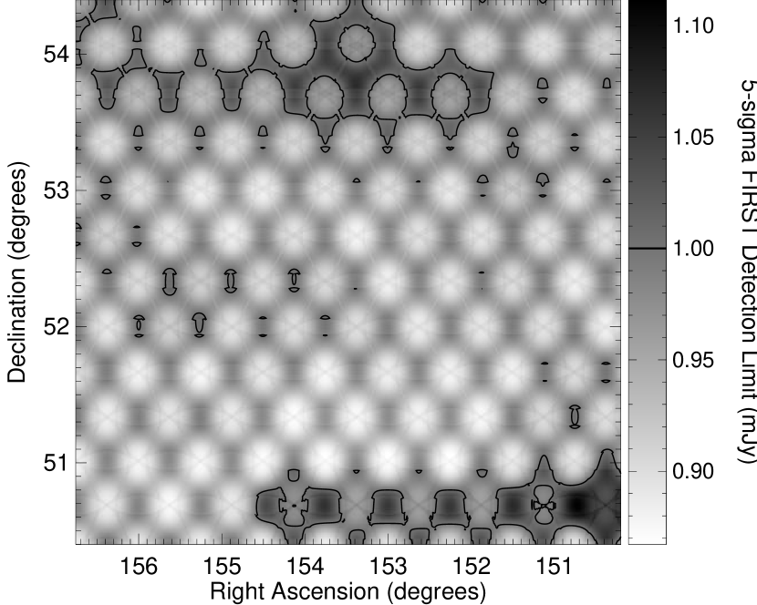
Figure 1: (a) Sensitivity of the FIRST survey as a function of position over the Deeprange area. The sensitivity varies slightly due to the hexagonal pointing pattern of the survey grid and due to the presence of bright sources that raise the noise level in the maps (see Becker, White & Helfand 1995 for more details.) A contour is drawn at 1 mJy, the flux density limit for the FIRST catalog. (b) Area covered by FIRST survey as a function of the $5\sigma$ 1.4 GHz detection limit. More than 90% of the Deeprange survey area is complete to 1 mJy, and 98.9% is complete to 1.05 mJy.

2.3 A Sample of Stellar Counterparts

We began our comparison of the radio and $I$-band data by deriving astrometric offsets between the two databases. Since the FIRST positions are tied to the ICRF (International Celestial Reference Frame; Ma et al. 1998) with an overall systematic bias of $<30$ mas (White et al. 1997), we adopt them as defining the reference frame for the match. A catalog of 978 radio/optical sources was constructed by matching the Deeprange catalog to both the FIRST catalog and a supplemental catalog based on VLA A-configuration observations of the Deeprange area. We corrected zero-point shifts in the astrometry for each CCD and derived a distortion correction for the intra-CCD positions in a manner analogous to our derivation of intraplate corrections for the APM survey (McMahon et al. 2002); these corrections were less than $1^{\prime\prime}$ peak-to-peak. Both stellar and non-stellar optical objects were included in the calibration; non-stellar objects have poorer positions but are much more frequent radio source counterparts, so they improve the overall calibration. The final registration of the two catalogs is accurate to $\sim 0.05^{\prime\prime}$ or better, and the rms scatter for individual sources is $1^{\prime\prime}$.

For the vast majority of the radio sources, we search for $I$-band counterparts by simply matching the positions. However, for multiple-component and extended radio sources, blind matching can lead to missed counterparts. Thus, maps were prepared for all objects by overlaying the radio contours on the $I$-band images; the maps were then examined by eye to select additional counterparts. Examples of these maps for the six classical Fanaroff-Riley Type II radio doubles (FRII – Fanaroff & Riley 1974) are shown in Figure 2. Four of these objects are quasars and two are galaxies. In three of these cases (including one quasar), a blind catalog match would not have found the counterpart to lie within $1.5^{\prime\prime}$ of an $I$-band source owing to the shifting of the centroid of the fitted Gaussian components by emission from along the radio jet, even though an obvious (and now confirmed) counterpart is present. Such cases are a source of modest incompleteness in any radio identification program that does not examine radio source morphology in detail (see, for example, Becker et al. 2001 for a test of the incompleteness of the FBQS arising from extended radio morphologies).

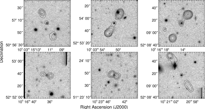
Figure 2: FIRST radio contours overlaid on Deeprange $I$-band images for six multiple component radio sources, including four quasars from Table 1 and two galaxies (bottom left and center panels) from Table 2. The contour levels are 1, 2, 3, 5, 10, 20, 50 and 100 mJy. Three of these objects (including the quasar at top center) would have been missed using a search algorithm that simply compares positions of the FIRST and Deeprange catalog sources.

Of the 617 FIRST radio sources with $I$-band counterparts coincident to within $1.5^{\prime\prime}$, 122 are classified as stellar. We calculate the expected chance coincidence rate using the number of stellar sources in an annulus between $5^{\prime\prime}$ and $12^{\prime\prime}$ around each radio source in the catalog. Among the 49 stellar counterparts brighter than $I=20.5$ we expect between 1 and 2 false matches. Another source of misidentification with stellar counterparts arises from galaxies misclassified as stars in the optical database; Postman et al. (1998) give an estimate of the magnitude-dependent rate at which this occurs. For $I<20.0$, we should expect 3 out of 41 such misclassifications, whereas for $20<I<21$ we estimate that nearly half of the putative stars are misclassified galaxies, and at fainter magnitudes the situation deteriorates rapidly. From these considerations, coupled with limitations imposed by the amount of spectroscopic confirmation time available, we have adopted a magnitude-limited threshold for $I$-band stellar counterparts of $I\leq 20.5$, leaving us 49 candidates of which we expect approximately $15\%$ to be either false or misclassified matches.

3 Spectroscopic Identification of Quasars in the Deeprange Field

Observations of the radio source counterparts were conducted over several observing sessions at the Keck II 10-m telescope using both the LRIS and ESI spectrographs. In general, the observing conditions were not photometric. All of the observations were taken at the parallactic angle to minimize slit losses. The LRIS data were reduced and spectra extracted using standard IRAF procedures. ESI spectra were produced using a combination of IRAF tasks and customized software developed by the authors. More details on the algorithms used in the ESI software are given in White et al. (2003).

We have obtained spectroscopic classifications for all of the 49 stellar radio source counterparts with $I<20.5$; one additional source slightly below this threshold was also observed. We find 35 quasars (see Table 1), one BL Lac object, two narrow-line AGN, six galaxies with H II-like spectra, five absorption-line galaxies, and one star. The definitions of the various classes are taken from FBQS2 and FBQS3: we define anything with broad lines as a quasar, objects with narrow emission lines as H II galaxies or AGN depending on their relative line strengths, and the single object with a featureless continuum as a BL Lac. One or more of the absorption-line galaxies could well contain nonthermal components (e.g., as do BL Lacs), but our discovery spectra are insufficient for quantitative classification.

Since only a tiny fraction of FIRST sources are actually identified with stars (Helfand et al. 1999b), the single stellar match almost certainly represents the expected one false coincidence (although the spectrum is unusually blue for a randomly selected star.) Likewise, the five galaxies along with some of the six H II galaxies comprise the expected number of $I$-band misclassifications, although in this case, they almost certainly do represent the optical counterpart to the radio source. The BL Lac, AGN, and the more luminous H II galaxies have sufficiently bright nuclei that their classification as stellar is to be expected. We summarize the optical and radio properties of the non-quasar sample members in Table 2. The spectra for the quasars and non-quasars are displayed in Figures 3 and 6, respectively.

Figure 3: Spectra of FIRST/Deeprange candidates identified as quasars, sorted by decreasing redshift. The dotted lines show expected positions of prominent emission lines: Ly$\alpha$ 1216, N V 1240, Si IV 1400, C IV 1550, C III] 1909, Mg II 2800, [O II] 3727, H$\delta$ 4102, H$\gamma$ 4341, H$\beta$ 4862, [O III] 4959, [O III] 5007, H$\alpha$ 6563. Note that some of the spectra have atmospheric A and B band absorption at $\sim 6880$ Å and 7620 Å.

Figure 3b: Continued. Spectra of FIRST/Deeprange quasars.

Figure 3c: Continued. Spectra of FIRST/Deeprange quasars.

Figure 6: Spectra of FIRST/Deeprange candidates identified as non-quasars, sorted by Right Ascension. The labelling is the same as Fig. 3.

Table 1 lists the parameters of the Deeprange radio quasar sample. The source coordinates from the Deeprange catalog are given in the first two columns, followed by the offset between the optical and radio positions. The peak 20 cm flux density of the source’s core component from the FIRST catalog and the total source size follow (col. 4 and 5). Major and minor axes derived from elliptical Gaussian fits are quoted if one component was sufficient to describe the source morphology; sources with major axes smaller than $2.5^{\prime\prime}$ are unresolved in the FIRST survey and their sizes are listed as upper limits. For multiple component sources, the full source extents were measured from the radio maps and are listed with a $``\sim``$ sign; classical FR II sources are marked with a T (for triple) or D (for double). The next column lists the FIRST catalog integrated flux densities for resolved single-component sources, and the sum of the flux densities for all multiple-component sources. (For unresolved sources, the peak and integrated flux densities are approximately equal, although noise can produce derived integrated flux densities somewhat below the peak values for weak sources; in these cases, the peak values are more reliable estimators.)

Column 7 lists the 20 cm flux density reported in the NRAO VLA Sky Survey (NVSS – Condon et al. 1998). The $45^{\prime\prime}$ beam of this survey is sensitive to low surface brightness emission that could be resolved out in the FIRST survey. Twenty-seven of the 35 quasars are detected in the NVSS; of the eight that lie below that survey’s threshold of 2.5 mJy, we examined the contour maps at the source locations and found four present at flux density levels between 1 and 2 mJy (indicated as, e.g., $\sim 1.4$). Comparing (as appropriate) the peak or integrated flux densities from FIRST with the NVSS values shows most sources agree to well within their combined uncertainties (systematic flux density uncertainties for the two surveys are $\sim 5\%$ in addition to the quoted statistical errors). Three of the point sources (FDQ J101308.8+505017, FDQ J102050.6+515719, and FDQ J102101.4+523956) could be variable by from 50% to a factor of two over the one- to three-year interval separating the two sets of observations although, given that the NVSS flux densities are higher in the first two cases, faint diffuse emission associated with the quasar could explain the discrepancies.

Column 8 lists the $I$-band magnitude for each quasar. These are followed by the magnitudes in the $F$ (red) and $J$ (blue) bands derived from the Guide Star Catalog (version 2.2.1) database. If the object is not present in this catalog, we record the APM POSS I $E$ (red) and $O$ (blue) magnitudes from the McMahon et al. (2002) FIRST optical identification catalog; three objects fall below the thresholds of both sets of plate scans and so are excluded from the color plots discussed below. Note that the POSS and $I$-band data are far from contemporaneous, and substantial source variability is possible, suggesting that the $I-$POSS colors are not highly reliable.

Columns 11 and 12 give $E(B-V)$, the reddening in the quasar rest frame, and $A(I)$, the extinction in the observed frame for the $I$-band, as determined from a fit to each spectrum. They are discussed in more detail below (§4.3).

The quasar redshift, plus comments on the source’s spectrum and its properties in other wavelength bands, complete the Table. Only one of the quasars (the optically brightest member of the sample, FDQ J101916.3+504557) has been reported prior to its FIRST detection (Stepanian et al. 1999); Gregg et al. (2000) earlier reported the discovery of the FR II BAL quasar FIRST J101614.2+520915. Three of these quasars are coincident with X-ray sources detected by ROSAT (but see below).

Most of the quasar spectra are unremarkable, although a few deserve comment:

FDQ J100353.6+515457 ($z=1.63$) — This object has an unusual spectrum with very broad Mg II emission and very strong Fe II emission.

FDQ J101204.0+531331 ($z=2.911$) — This quasar’s emission lines have substantially lower equivalent widths than the FBQS composite spectrum (Brotherton et al. 2001).

FIRST J101614.2+520915 ($z=2.43$) — As was discussed in Gregg et al. (2000), this object is a high ionization broad absorption line quasar (HiBAL) with an FRII radio morphology, conclusively demonstrating that BALs can be radio loud.

FDQ J101735.0+533535 ($z=3.27$) — This is a low ionization broad absorption line quasar (LoBAL) based on the presence of broad absorption by both C IV and Al III.

FDQ J101742.7+535635 ($z=1.40$) — This quasar has very strong absorption lines due to Mg II and Fe at a redshift of $z=1.305$, indicative of an intervening damped Lyman alpha line system (Rao & Turnshek 2000).

FDQ J101939.9+514924 ($z=1.502$) — This quasar’s emission lines are unusually strong (or its continuum weak) compared with the FBQS composite spectrum.

FDQ J102223.9+523842 ($z=1.857$) — This appears to be a HiBAL as well, albeit a marginal example of one.

FDQ J100632.3+534852 ($z=1.040$),

FDQ J101119.2+520536 ($z=0.901$),

FDQ J101316.8+511118 ($z=1.16$),

FDQ J102007.2+522445 ($z=1.225$),

FDQ J102132.2+511433 ($z=0.944$) — These quasars all have red spectra. They are discussed further below (§4.3).

4 Discussion

Our spectroscopic campaign has resulted in the discovery of 35 quasars. One might wonder whether it is worthwhile to create a new, small sample of quasars even as large quasar surveys from the Sloan Digital Sky Survey and 2dF are producing samples with thousands or tens of thousands of objects. We believe that this and similar focused studies continue to be interesting because they explore new parts of parameter space. The SDSS/FIRST sample (Ivezić et al. 2002) currently includes 441 spectroscopically confirmed quasars with $i^{*}<18.5$ over 1030 deg² of sky. It is therefore 2 magnitudes brighter than this paper’s sample. As a result it is less dense on the sky by a factor of 5, and it includes only the bright end of the quasar luminosity distribution (as does the FBQS2 sample). Consequently the SDSS/FIRST redshift distribution is much more heavily dominated by low-redshift objects.

On the other hand, the 2dF QSO Redshift Survey (Croom et al. 2001) is deep ($18.25<b_{J}<20.85$), and includes $\sim 11000$ quasars spread over 289.6 deg². Presumably about 10% of these would be detected by a 1 mJy radio survey like FIRST (although only the northern equatorial strip is actually covered by FIRST); the 2dF sample thus includes about 3.8 FIRST quasars deg^-2, a slightly higher density than the sample reported here. But the 2dF survey is expected to be complete only for $0.3<z<2.2$ and detects no quasars with $z>3$. In contrast, in our 35 object sample we detect two $z>3$ quasars. Since it is a survey defined from a blue magnitude, the 2dF catalog is also biased against the inclusion of red objects. As we show below, 2dF, and most previous quasar surveys, have missed a large population of red objects.

4.1 Redshift Distribution

The limiting $I$ magnitude of 20.5 for this sample is nearly 3 magnitudes fainter than the limit in the FBQS1&2, and 1.5 magnitudes deeper than the limit in FBQS3. The samples do show some distinct differences, perhaps the most pronounced being in the redshift distribution. Continuing a trend discernible in comparisons between FBQS2 and FBQS3, as one goes to fainter magnitudes a significant deficit of low redshift quasars develops, to the extent that, in the Deeprange sample, there are very few quasars below a redshift of 1 (see Fig. 7). The lack of low-redshift quasars results mainly from the small volume being sampled (Fig. 8) combined with the excellent sensitivity of the survey, which is capable of detecting even low-luminosity quasars for $1<z<2$ where there are far more quasars than at lower redshifts.

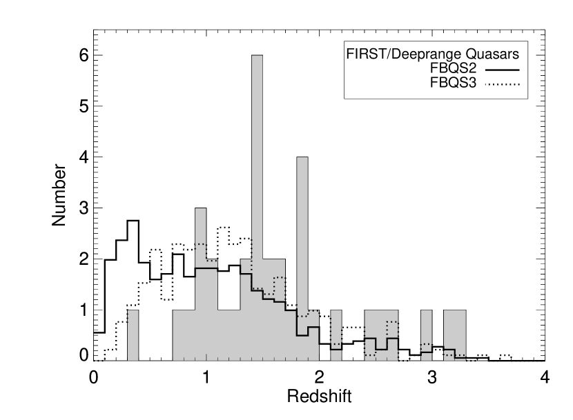
Figure 7: Redshift distribution for FIRST/Deeprange quasars (shaded) compared with distributions for the FBQS2 (solid; White et al. 2000) and FBQS3 (dotted; Becker et al. 2001) samples normalized to the same total counts. The FDQ sample contains many fewer low redshift quasars. The narrow peaks at $z=1.45$ and 1.85 are also striking.

Figure 8: Distribution of FDQ quasars in comoving spatial coordinates. Distances were calculated using a cosmological model with $H_{0}=70$, $\Omega_{M}=0.3$, and $\Omega_{\Lambda}=0.7$. The tangential distance is measured in the RA direction (so declination is normal to the page.) The paucity of quasars at redshifts less than 0.8 is due both to the limited volume covered by the survey and to the rapid increase in the quasar number density at $z\sim 1$.

It is possible the requirement that the $I$-band images to appear point-like causes us to miss some lower luminosity AGN at low redshifts because their host galaxies are also detected. However, the number of such objects is not expected to be very large. From the FBQS catalog, we expect to find $\sim 1.4$ quasars with $F\leq 17.8$ and $z<0.7$ in the FDQ survey area; the FBQS3 catalog predicts $\sim 1.7$ quasars with $F<18.9$. The single $z<0.7$ quasar we detect is not much below expectations given the slowly rising counts for low redshift AGN.

The narrow peaks at $z\sim 1.5$ and 1.9 in the redshift distribution are notable. They are created by groups of a few objects (also visible in Fig. 8) with characteristic pair separations of $\sim 60h^{-1}$ Mpc. Possible quasar clustering on similarly large scales has been reported before (e.g., Graham, Clowes & Campusano 1995; Komberg, Kravtsov, & Lukash 1996). The statistical evidence for clustering in this small sample is fairly weak using conventional measures of clustering; we defer the complete analysis of the clustering properties of this and other radio quasar samples to another paper.

4.2 Broad Absorption Line Quasars

One of the more interesting results to come out of the FBQS was the large number of BALQSOs in the radio-selected sample. While traditional blue-selected samples contain 10% BALQSOs, the FBQS contains 18%. It is unsurprising, then, that this radio-selected Deeprange sample also contains a relatively high fraction of BALQSOs. Out of nine quasars at a sufficiently high redshift to allow a C IV BAL to be seen, three are BALQSOs (33%). Although this is a small sample, it does add weight to the conclusion that, contrary to some earlier work, radio-intermediate quasars are more likely to be BALQSOs than radio quiet quasars; equally important, this sample of 35 quasars includes the first example of a radio-loud FR II BAL quasar (Gregg et al. 2000).

4.3 Colors for Faint $I$-band Selected Quasars

The median $O-E$ colors (roughly equivalent to $B-R$) for FBQS2 and FBQS3 quasars with $z>0.4$ are 0.52 and 0.63, respectively, for survey limits of $E=17.8$ and $E=19.0$. For the current survey limit of $I=20.5$ we might expect the median to be another $\sim 0.1$ magnitude redder, but the observed median for the 27 $z>0.4$ Deeprange quasars with both colors shows an increase more than three times this large: $J-F=0.84$. The comparison is displayed graphically in Figures 9 and 10. A two-sided Kolmogorov-Smirnov test indicates that the FDQ and FBQS2 distributions are different with 99.94% confidence, while the FDQ and FBQS3 distributions differ with 97.8% confidence.

The mean and median $J-F$ colors are identical for the $z<2$ FDQ quasars and for the entire FDQ sample. The redder colors are therefore not a consequence of the higher mean redshift of the $I$-band sample (Fig. 11). The color difference is also not the result of the various red and blue bands employed in the different surveys. The $J$ and $F$ bands are slightly redder than the $O$ and $E$ bands, extending about 30 nm farther to the red in each case. Consequently $J-F<O-E$ for the reddest objects. Thus by comparing the $J-F$ colors for the FDQ sample directly with $O-E$ for the FBQS samples, we get a conservative estimate of the color difference between the samples; the actual color difference will be larger (by up to 0.5 mag) for the reddest objects.

It appears that the quasars are redder both because of the fainter optical magnitude limit and as a result of being selected in a redder band. This is consistent with the result expected if dust extinction is relevant: a quasar of a given intrinsic luminosity with extra dust will be both fainter and redder. Ignoring such effects can lead to a serious underestimate of the size of the red quasar population.

Figure 9: Cumulative color distributions for FIRST/Deeprange quasars (solid), FBQS2 (dashed) and FBQS3 (dotted). The FDQ sample is noticeably redder than the other samples (which were selected using $R$ magnitudes instead of $I$ as in the FDQ sample.)

Figure 10: Colors of FDQ quasars (large symbols) and FBQS2/FBQS3 quasars (small symbols) as a function of red magnitude. The error bars for the four brighter bins show the mean and error in the mean for the FBQS quasars over the magnitude range. The faintest bin shows the mean for the FDQ quasars. There is a slight trend toward redder colors at fainter magnitudes in the FBQS samples, but the FDQ sample is significantly redder than the extrapolation of that trend. Note that this diagram omits seven FDQ sources that are undetected in one or both optical colors; the spectra show six of them to be quite red.

Figure 11: Colors of FDQ quasars (large symbols) and FBQS2/FBQS3 quasars (small symbols) as a function of redshift. The error bars show the mean and rms for the FBQS quasars in redshift bins. The FDQ sample is somewhat redder than the FBQS, but the difference does not depend strongly on redshift.

In addition to the redder mean color of the sample, the removal of the color cut (at $O-E<2.0$) has allowed us to identify three objects too red to be included in the FBQS. One of these is a low-ionization BAL (FDQ J101735.0+533535, $z=3.270$), but the other two simply have red spectra (in Fig. 3, see FDQ J102007.2+522446, $z=1.225$, and FDQ J101119.3+520537, $z=0.901$.) The $J-F$ colors for these three objects, estimated from the spectra using synthetic photometry, are 2.3, 2.6 and $>3$ respectively. A fourth object with a similarly red spectrum, FDQ J100632.4+534852 ($z=1.040$), formally fails to exceed the color cut, but lacks simultaneous red and blue magnitudes which would probably show that it too would have failed to be included in the FBQS sample; its synthetic $J-F$ is 2.5. Thus, $\sim 10\%$ of the quasars confirmed here would have been missed in a radio-selected sample even when the color cut is more than a magnitude redder than the sample mean.

Are these red spectra the result of extinction by dust? To estimate the reddening for our quasars, we have fitted the spectra using the FBQS composite spectrum (Brotherton et al. 2001) with a Small Magellanic Cloud (SMC) dust reddening law from Gordon & Clayton (1998). The SMC extinction rises steeply into the ultraviolet (making it possible to produce red spectra with less visual extinction) and lacks the 2175 Å bump seen in Galactic dust. The SMC law is similar to dust observed in energetic extragalactic sources such as quasars and starbursts; no quasar has been seen to have a 2175 Å absorption bump (Pitman, Clayton, & Gordon 2000). We have not attempted to fit the spectra for the two quasars that have strong broad absorption line systems, since those objects are heavily reddened by the BALs themselves. Table 1 gives the results determined from these fits: $E(B-V)$, the reddening in the quasar rest frame, and $A(I)$, the $I$-band extinction in the observed frame.

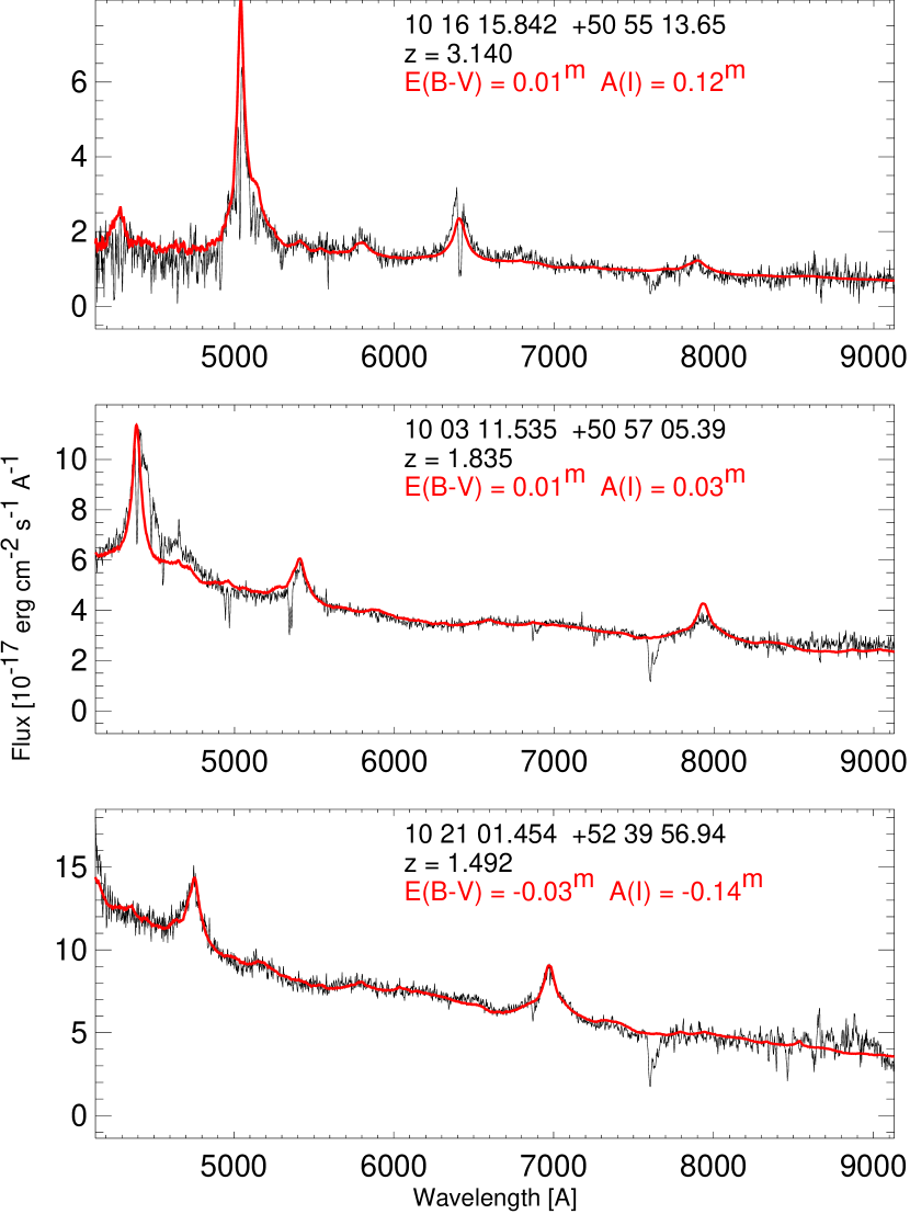
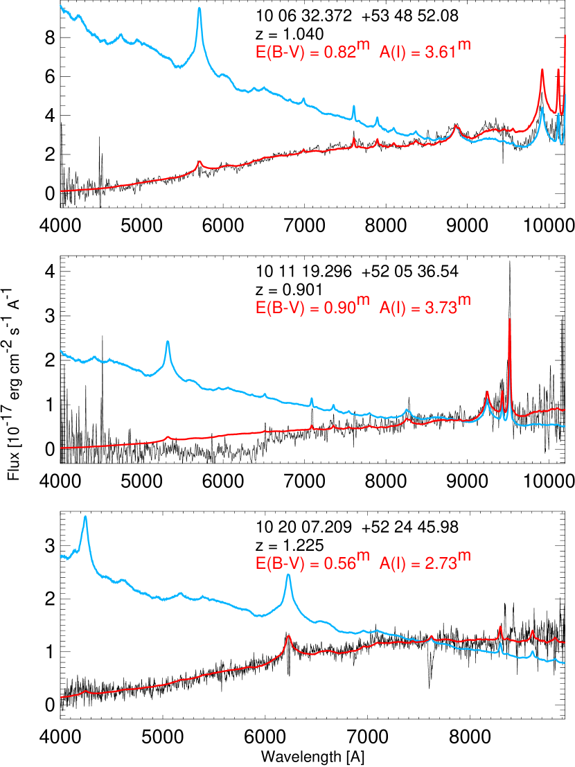
(a)	(b)

Figure 12: Results of fitting the FBQS composite spectrum (Brotherton et al. 2001) reddened with an SMC extinction law (Gordon & Clayton 1998) to the FDQ spectra. (a) Fits to three selected quasars with typical spectra having little reddening. The $E(B-V)$ and $I$-band extinction $A(I)$ are given. The reddening is allowed to be negative in the fit since the FBQS composite itself could include a small amount of extinction. (b) Fits to the three very red quasars. The unreddened composite spectrum, matched to the red half of the data, is also shown. The fits to FDQ J100632.3+534852 (top) and J102007.2+522445 (bottom) are excellent; the fit to J101119.2+520536 is good, but the observed spectrum has an unexplained break at 6500 Å. The extinction for these quasars is large.

Figure 13: Distribution of fitted values for $E(B-V)$ dust reddening. Quasars with red colors due to broad absorption lines rather than dust have been omitted. All other red quasars are seen only at relatively low redshifts, $z<1.3$. The lack of blue light in their spectra makes more distant examples too faint to detect in the $I$-band.

As can be seen from the examples in Figure 12(a), most of the quasars are excellent fits to the template spectrum with little or no reddening, but a minority show evidence for quite large extinction values (Fig. 12b). The reddened models fit the observed spectra well; note that both the continuum and broad emission lines are well matched by the model.

One might be tempted to assume that because the red quasars represent only a small fraction of the sample, they are also a small fraction of the quasar population. However, Figure 13 shows a very interesting correlation: all of the red quasars are found at relatively low redshifts. Five of the ten quasars with $z<1.3$ have very red colors. A two-sided Kolmogorov-Smirnov test indicates that the redshift distributions of red quasars (with $E(B-V)>0.5$) and non-red quasars differ at the 96.5% confidence level.

Figure 14: Dereddened $I$-band absolute magnitudes as a function of redshift. The five red quasars with observed $E(B-V)>0.2$ are indicated by filled symbols. The dashed lines show our $I<20.5$ detection limit as a function of the amount of reddening, $E(B-V)$. Even the most luminous quasars are undetectable in the $I$-band at redshifts $z>1.5$ in the presence of $E(B-V)=0.75$ magnitudes of reddening. We are likely to be detecting only the most luminous tip of the red quasar iceberg.

Red quasars are not seen at higher redshifts because their red colors make them very difficult to detect there. As the redshift increases and bluer rest wavelengths shift into the $I$-band, such objects quickly fade to the point of invisibility. We have computed synthetic $I$ magnitudes as a function of redshift for our sample spectra to determine the limit of visibility ($I<20.5$) for each source. Distances were computed using a $\Lambda$-cosmology with $H_{0}=70$, $\Omega_{m}=0.3$, and $\Omega_{\Lambda}=0.7$. The results for the ten $z<1.3$ quasars are given in Table 3. If the red quasars that we observe were moved to $z=1.5$, none of them would have been detectable above the $I<20.5$ limit of our survey. In contrast, the low-redshift blue quasars detected in our sample are visible to much greater redshifts, typically $z=1.7$–2.1. Unless red quasars are preferentially found only at low redshifts — and it is just a matter of luck that our detection limit forbids us from detecting more distant objects — there must be many more red quasars associated with the quasar population peak at $1<z<2$.

The excellent fits to the spectra in Figure 12(b) argue strongly in favor of dust as the source of the reddening for at least some of our red quasars. In that case the implied dereddened luminosities are large. Even with a magnitude limit $I<20.5$, our survey is deep enough to detect only the most luminous of these reddened quasars. Figure 14 shows the dereddened $I$-band absolute magnitudes as a function of redshift along with the effect of reddening on our detection limit. For higher redshift objects where bluer rest wavelengths move into the $I$-band, even a small amount of dust absorption has a dramatic effect on detectability. The only objects detectable at a reddening as large as $E(B-V)=0.7$ are the three quasars that are actually seen to be very red (Fig. 12b), and it would be impossible to detect similar objects in the $I$-band at redshifts greater than $\sim 1.5$. The five most luminous objects with $z<1.3$ are all red.

Unless highly reddened quasars are also preferentially highly luminous, there must be an even larger, as yet undiscovered, population of quasars at lower luminosity. Such a correlation is not completely implausible; perhaps quasars that are heavily reddened have just accreted a new source of fuel that guarantees they will also be relatively luminous. Since the luminosity cannot exceed the Eddington limit, however, we still expect to find lower luminosity reddened quasars associated with lower black hole masses.

This conclusion appears difficult to escape. For some quasars, an optical synchroton emission component or contaminating light from a host galaxy can produce a redder spectrum (Benn et al. 1998; Whiting, Webster & Francis 2001). Our red quasars with lower $E(B-V)$ values might be fitted with a red synchrotron continuum. However, any explanation of the reddest quasars based on an additional emission mechanism is strongly ruled out by our observations. Not only are the reddened quasar template spectra generally a good fit to our data, but the quasar light must be strongly suppressed in the ultraviolet to explain the absence of red quasars at higher redshifts from our sample.

Our data strongly support the hypothesis, originally raised by Webster et al. (1995) based on a radio sample with a much higher ($\sim 100$ mJy) flux density threshold, that radio quasars are dominated by a previously undetected population of red, heavily obscured objects (see also Srianand & Kembhavi 1997; Benn et al. 1998; Kim & Elvis 1999). The red objects we detect represent fully half the population of the $z<1.3$ quasars in our sample; unless their underlying luminosity and redshift distributions are very different than those of blue quasars, there must be many more such objects at higher redshifts and lower luminosities comparable to our blue quasars. We are likely to be detecting only the most luminous tip of the red quasar iceberg.

5 Associations Between Quasars and Clusters

We have compared the positions of the objects in our sample to the catalog of cluster candidates in Postman et al. (2002). Eight sources lie within $2.5^{\prime}$ of a cluster centroid, with an expected chance coincidence rate of five matches (ignoring the small overlap of cluster candidates). Five of the cluster/radio-source coincidences are matches between rarer high-redshift cluster candidates and confirmed quasars. A $2.5^{\prime}$ radius around the $z\geq 0.8$ clusters covers only 3.7% of the survey area, so that only 1.3 chance coincidences with quasars would be expected. In addition, three of the matching quasars have redshifts similar to the estimated cluster redshifts: cluster #243 ($z\sim 1.1$) with FDQ J101510.6+523643 ($z=0.960$), cluster #304 ($z\sim 0.8$) with FDQ J101119.2+520536 ($z=0.901$), and cluster #382 ($z\sim 0.8$) with FDQ J101002.1+512700 ($z=0.787$). It is likely that all three are real associations that confirm the cluster redshift estimates.

Two of the three quasars coincident with X-ray sources are also close to cluster candidates, and it is possible that a hot intracluster medium is responsible for the X-ray emission; in the case of cluster #34 ($z\sim 0.3$) and FDQ J102256.6+540717 ($z=0.340$), the cluster and quasar redshifts match, and a physical association is quite probable.

There are only two other FDQ quasars with redshifts less than unity, and one of them also has a cluster match, albeit at a slightly greater separation. Cluster #303 ($z\sim 0.7$) is $3.0^{\prime}$ from FDQ J102059.8+520917 ($z=0.813$). The close agreement in the redshifts makes this another likely physical association.

This is a remarkable result: five of the six $z<1$ quasars in the FDQ are associated with Deeprange cluster candidates of similar estimated redshifts. Despite the large number of candidates (444) in the cluster catalog, this is highly statistically significant. Using a radius of $3^{\prime}$, the cluster candidates cover 22% of the survey area, so the probability that five of six $z<1$ quasars lie within $3^{\prime}$ of a cluster of any redshift is only $2\times 10^{-3}$. The probability that five randomly selected clusters will all have redshifts within $\pm 0.15$ of the five $z<1$ quasar redshifts is even smaller, only $\sim 5\times 10^{-4}$. The joint probability of both happening by chance is very small, even considering the a posteriori nature of this argument.

The only $z<1$ quasar without an associated cluster is FDQ J102132.2+511433 ($z=0.944$). The Deeprange cluster selection efficiency is expected to decline at such high redshifts (Postman et al. 2002), so we would not expect all $z\sim 0.95$ clusters to be included in the Deeprange catalog. Our results are therefore consistent with the possibility that all of our $z<1$ quasars are associated with clusters.

This has some surprising implications. Recall that only 10% of quasars are radio-loud (RLQs); there must be $\sim 300$ additional radio-quiet QSOs (RQQs) with $I<20.5$ in the Deeprange area. Since 3 of the 109 $z\geq 0.8$ Deeprange cluster candidates have associated RLQs, one can project that $\sim 30$ such clusters will have an associated quasar when the RQQs are included. Since 30–40% of the $z\geq 0.7$ cluster candidates are expected to be spurious (Postman et al. 2002), that would lead to half of the real high-redshift cluster candidates having associated quasars.

Another possibility, however, is that the RLQs are preferentially found in clusters and that the (as yet undiscovered) RQQs in this field will not be associated with Deeprange clusters. Many studies have concluded that RLQs are more likely to be found in high-density cluster environments than are RQQs (e.g., Yee & Green 1984; Ellingson, Yee & Green 1991) although others have concluded that RQQs and RLQs are both found in clusters (e.g., Hutchings, Crampton & Johnson 1995; Wold et al. 2001). Recently Söchting, Clowes, & Campusano (2002) explored the correlation between clusters and RQQs at $z\sim 0.3$ and found that the RQQs do associate with clusters but that they tend to occupy the cluster periphery rather than the cluster core. Note that some of the five FDQ quasars are also relatively far from the cluster centers, with projected local distances of 0.4–1.5 Mpc.

Quasar/cluster associations have generally not been analyzed at $z\sim 1$ because it is difficult to identify clusters at such high redshifts. Since quasars were far more common at $z\sim 1$ than at $z\sim 0.3$, it is expected that more clusters will have quasars at high redshifts. Whether as many as half the $z\sim 1$ clusters have associated quasars, as we suggest, can be confirmed by future studies. The Deeprange field would be a fruitful target for searches for radio-quiet quasars in order to quantify this association. Spectroscopic redshifts for the associated cluster candidates will also help confirm their association with FDQ quasars.

6 Summary and Conclusions

A complete, magnitude-limited sample of radio-emitting quasars in the Deeprange I-band survey has been constructed by obtaining optical spectra for 50 stellar counterparts to FIRST radio sources in the 16 deg² survey region. Thirty-five quasars were detected. In addition to the first radio-loud FRII BAL quasar, two additional BAL quasars were discovered, representing fully one-third of objects with a high enough redshift for the BAL signature to be seen. A probable damped-Lyman-alpha absorber was identified in another source. Most intriguing, however, is the discovery of five very red quasars with $0.7<z<1.3$ that represent half of all objects in this redshift range. Indeed, if we use dereddened magnitudes, the five most luminous quasars with $z<1.3$ are all red, and three of the six most luminous objects in the entire 35-member sample are red. Fits of the FBQS composite quasar spectrum with an SMC reddening law yield $I$-band extinctions of $1.2<A(I)<3.7$ magnitudes for the five reddest quasars.

We show that with reddenings this large, even the most luminous quasars ($M_{B}<-27$) are not detectable beyond $z=1.5$ at our $I$-band magnitude limit of 20.5. Indeed, the combination of the good fits of the reddened composite spectrum to our spectra and the absence of any red quasars at higher redshift (naturally attributable to extinction) strongly suggest that 1) the quasars are red because of dust, and 2) the detected objects represent only a small fraction of the total population.

This striking support for the Webster et al. (1995) results on the missing red quasar population, using the much larger population of objects with radio fluxes several hundred times fainter, is cause for reflection. Are the most luminous quasars red because they are both magnified and reddened by an intervening galaxy? Gregg et al. (2002) argued that this could explain the red quasars found in a survey of FIRST-2MASS counterparts, and several other examples are known of very red quasars that are lensed (Hewitt et al. 1992, Courbin et al. 1998). An argument that weighs heavily against this hypothesis is that the lensing fraction would be absurdly high. If most lensed quasars are missed because they are reddened, it is in principle possible that we have the lensing fraction wrong; however, cosmological constraints strongly reject the possibility that the lensing fraction is as high as 10%. A high lensing fraction in objects selected to be very red is allowed since that sample could be strongly biased, but the sample presented in this paper has no color bias (for either red or blue objects) so it should not have any particular bias toward lensed objects.

Could the dust fraction increase with cosmic time (along with metallicity) so that moving out beyond $z=1.3$ will not yield a significant additional population of reddened quasars? Possibly, although there is little evidence from quasar spectra for metallicity evolution out to $z>6$; it is more likely that dust gets destroyed and/or blown away as a quasar ages and undergoes repeated high luminosity intervals, so that there might well be fewer reddened objects at low redshift.

It remains unknown whether or not the large number of hidden quasars adduced from first the radio-loud and now the radio-intermediate segments of the population extends to radio-quiet objects. We note that the radio flux distribution for the red quasars is indistinguishable from that for the other quasars in our sample, and that two of the red quasars have flux densities close to the FIRST detection limit. It is therefore unlikely that such objects are found only in radio sources with $F_{\nu}>1$ mJy. Addressing the question of whether red quasars are common in the radio-quiet population is clearly of considerable importance for assessing the true accretion luminosity of the Universe and its evolution with cosmic time.

Finally, we have found that five of the six quasars in our sample with $z<1$ are associated with Deeprange cluster candidates with concordant redshift estimates. Extrapolating these results to the radio-quiet portion of the population suggests that up to half of the $0.3<z<1$ clusters have associated quasars. Spectroscopic redshifts for the cluster galaxies and a search for radio-quiet quasars in this field are required to confirm this suggestion.

Table 1: Spectroscopically Confirmed Quasars in the Deeprange Field

RA	Dec	Offset	$F_{pcore}$	Size	$F_{int}$	NVSS	$I$	$F$	$J$	$E(B{-}V)$	$A(I)$	$z$	Comments
(2000)	(2000)	(′′)	(mJy)	(′′)	(mJy)	(mJy)	(mag)	(mag)	(mag)	(mag)	(mag)
(1)	(2)	(3)	(4)	(5)	(6)	(7)	(8)	(9)	(10)	(11)	(12)	(13)	(14)
10 01 30.555	+53 31 51.02	0.49	4.0	$3.1\times 2.5$	5.1	$4.2\pm 0.4$	19.74	$>20.4$	20.84	$-0.04$	$-0.29$	2.192
10 01 32.427	+51 29 54.52	2.06	1.4	$4.4\times 0.0$	1.8	$<1.4$	19.06	19.84	20.54	$-0.05$	$-0.24$	1.094
10 02 40.947	+51 12 45.36	0.83	3.8	$<2.5$	$\cdots$	$4.0\pm 0.4$	20.34	$>20.4$	21.44	$-0.04$	$-0.24$	1.80	close pair; poss. damped Ly$\alpha$, $z=0.99$ Mg II
10 03 11.535	+50 57 05.39	1.44	1.6	$\sim 55T$	24.3	$24.2\pm 1.2$	19.33	18.98	19.93	$0.01$	$0.03$	1.835	close pair; poss. damped Ly$\alpha$, $z=0.91$ Mg II
10 03 50.707	+52 53 52.41	13.08	6.9	$\sim 55T$	113.0	$114.8\pm 3.8$	18.52	18.58	19.59	$-0.02$	$-0.09$	1.33
10 03 53.654	+51 54 57.29	0.50	1.1	$6.3\times 0.0$	1.5	$<1.4$	18.26	18.85	19.88	$0.12$	$0.70$	1.63	v. broad Mg II; strong Fe II
10 04 00.401	+54 16 16.96	0.83	9.0	$<2.5$	$\cdots$	$7.1\pm 0.5$	18.84	19.17	20.52	$0.06$	$0.31$	1.48
10 06 32.372	+53 48 52.08	0.34	1.3	$3.0\times 0.0$	1.4	$4.8\pm 0.5$	19.22	20.40	22.15	$0.82$	$3.61$	1.040	very red; confused &/or extended ($F_{int}=3.9$ mJy)
10 08 08.472	+50 43 21.36	0.17	17.0	$<2.5$	$\cdots$	$17.3\pm 0.6$	19.57	19.50	20.06	$0.03$	$0.14$	1.43
10 09 04.530	+52 44 17.37	2.03	1.9	$13.8\times 4.3$	8.7	$7.6\pm 0.5$	19.79	19.58	20.70	$-0.02$	$-0.10$	1.45
10 10 02.117	+51 27 00.20	1.21	1.4	$3.7\times 1.1$	1.8	$\sim 2.0$	18.01	18.38	18.44	$-0.07$	$-0.29$	0.787
10 10 39.305	+51 31 09.04	0.64	11.3	$<2.5$	$\cdots$	$12.3\pm 0.5$	20.00	19.81	20.82	$-0.03$	$-0.24$	2.562
10 11 19.296	+52 05 36.54	0.72	1.2	$<2.5$	$\cdots$	$3.1\pm 0.5$	20.00	$>20.4$	$>22.4$	$0.90$	$3.73$	0.901	very red
10 12 04.077	+53 13 31.91	0.36	3.5	$<2.5$	$\cdots$	$7.0\pm 1.4$	18.54	18.88	19.57	$0.02$	$0.15$	2.911	$\sim 100^{\prime\prime}$ extent in NVSS; very weak lines
10 13 08.804	+50 50 17.68	0.45	9.0	$<2.5$	$\cdots$	$13.4\pm 0.9$	19.34	19.78	20.15	$-0.03$	$-0.21$	1.817	$\sim 26^{\prime\prime}$ extent in NVSS; Mg II abs
10 13 16.827	+51 11 18.06	0.77	18.4	$<2.5$	$\cdots$	$16.0\pm 0.6$	19.87	$>20.4$	$>22.4$	$0.26$	$1.20$	1.16	red; low S/N spectrum
10 14 09.896	+51 52 28.67	1.20	3.1	$<2.5$	$\cdots$	$\sim 2.0$	19.54	19.79	20.36	$0.01$	$0.06$	1.775
10 15 10.623	+52 36 43.22	0.20	4.7	$3.7\times 1.2$	5.8	$6.8\pm 0.5$	20.15	20.45	22.04	$0.10$	$0.44$	0.960
10 16 14.223	+52 09 15.68	0.30	5.2	$\sim 62T$	176.9	$185.2\pm 6.0$	18.68	19.19	20.92	$\cdots$	$\cdots$	2.43	FRII HiBAL; weak emission lines
10 16 15.842	+50 55 13.65	0.29	27.8	$<2.5$	$\cdots$	$26.8\pm 0.9$	20.25	20.39	21.07	$0.01$	$0.12$	3.14	strong rest C IV abs
10 17 35.005	+53 35 35.49	0.44	1.8	$2.8\times 0.0$	1.9	$\sim 2.0$	19.39	$>20.4$	$>22.4$	$\cdots$	$\cdots$	3.27	bright foreground cluster; spectacular LoBAL
10 17 42.660	+53 56 35.50	0.76	67.8	$3.8\times 1.2$	85.2	$92.9\pm 2.8$	18.43	18.67	19.72	$0.05$	$0.29$	1.40	poss. damped Ly$\alpha$, $z=1.305$ Mg II
10 18 57.724	+53 34 13.49	0.32	8.9	$<2.5$	$\cdots$	$7.9\pm 0.5$	19.59	19.83	20.78	$-0.03$	$-0.16$	1.495
10 19 16.385	+50 45 57.50	0.30	1.9	$4.8\times 3.2$	2.9	$4.5\pm 0.5$	17.37	17.29	18.07	$0.00$	$0.01$	1.311
10 19 39.990	+51 49 24.04	0.51	3.6	$<2.5$	$\cdots$	$3.8\pm 0.4$	20.54	19.93	20.19	$0.07$	$0.38$	1.502	note $I>20.5$; faint continuum
10 20 07.209	+52 24 45.98	0.96	6.5	$2.7\times 1.3$	7.5	$6.8\pm 0.5$	19.74	19.89	$>22.4$	$0.56$	$2.73$	1.225	very red
10 20 50.635	+51 57 19.01	0.52	1.9	$<2.5$	$\cdots$	$4.4\pm 0.5$	19.41	19.65	20.49	$0.06$	$0.34$	1.63	unrelated source $12^{\prime\prime}$ away
10 20 59.887	+52 09 17.87	0.60	1.4	$\sim 120T$	35.1	$34.0\pm 1.5$	18.67	18.88	19.63	$0.01$	$0.02$	0.813
10 21 01.454	+52 39 56.94	0.22	3.8	$<2.5$	$\cdots$	$<1.4$	18.65	18.58	19.39	$-0.03$	$-0.14$	1.492	PSPC=0.010
10 21 32.233	+51 14 33.80	0.24	63.7	$3.2\times 1.0$	75.1	87.0	19.91	$>20.4$	21.44	$0.40$	$1.60$	0.944	red; core-jet source; PSPC = 0.008
10 22 23.869	+52 38 42.50	0.60	6.3	$<2.5$	$\cdots$	$7.2\pm 0.4$	18.83	19.48	20.71	$0.01$	$0.05$	1.857	HiBAL
10 22 56.641	+54 07 17.95	0.41	1.2	$<2.5$	$\cdots$	$\sim 1.4$	18.09	17.97	19.25	$0.04$	$0.11$	0.340	RASS=0.024
10 23 52.706	+54 06 49.63	0.77	1.6	$<2.5$	$\cdots$	$<1.4$	19.96	20.30	21.22	$-0.04$	$-0.24$	1.95
10 24 22.390	+51 38 38.77	0.78	2.2	$6.6\times 3.5$	4.1	$5.1\pm 0.4$	19.42	20.24	20.80	$-0.04$	$-0.24$	1.518	6.15mJy with 2nd source $25^{\prime\prime}$ away
10 26 27.697	+51 41 14.49	0.53	5.5	$<2.5$	$\cdots$	$6.6\pm 0.4$	18.54	19.23	19.71	$-0.01$	$-0.10$	2.63	27mJy @6cm $\rightarrow$ inverted spectrum

Table 2: FIRST Deeprange Sample Non-Quasars

RA	Dec	Offset	$F_{\rm pcore}$	Size	$F_{\rm int}$	NVSS	$I$	$z$	Comments
(2000)	(2000)	(′′)	(mJy)	(′′)	(mJy)	(mJy)	(mag)
(1)	(2)	(3)	(4)	(5)	(6)	(7)	(8)	(9)	(10)
10 00 40.735	+53 19 11.69	0.27	2.7	$<2.5$	$\cdots$	3.0	18.77	$\cdots$	BL Lac object
10 01 34.174	+50 43 37.98	1.46	2.6	$4.4\times 0.0$	3.0	3.8	18.61	0.39	Galaxy
10 01 52.743	+52 46 13.43	0.48	1.1	$<2.5$	$\cdots$	$<1$	20.09	0.56	H II Galaxy
10 02 53.517	+51 37 08.56	1.20	1.4	$<2.5$	$\cdots$	$\sim 1$	17.08	0.25	H II Galaxy
10 03 25.102	+51 01 18.76	0.37	1.6	$<2.5$	$\cdots$	$\sim 1$	20.26	0.66	H II Galaxy (surrounding cluster)
10 04 27.868	+54 11 55.93	1.07	1.8	$6.6\times 4.2$	3.7	2.3	19.55	0.45	H II Galaxy
10 05 12.387	+54 32 40.99	0.32	1.4	$>400$	40.2	121-177	19.27	0.49	H II Galaxy
10 11 45.770	+51 28 49.82	1.07	1.2	$7.3\times 1.4$	2.2	$\sim 1$	19.77	0.69	Galaxy
10 12 33.446	+53 07 02.08	0.53	1.7	$<2.5$	$\cdots$	4.2	19.35	0.00	Star
10 14 43.644	+51 23 44.34	0.10	2.6	$<2.5$	$\cdots$	2.5	17.08	0.30	Galaxy
10 16 36.503	+52 52 37.76	5.94	$\cdots$	$\sim 15$	10.0D	10.1	19.99	$\sim 0.90$	Galaxy
10 23 08.712	+52 47 40.18	0.64	1.6	$4.5\times 0.0$	2.0	$\sim 1$	20.36	0.93	H II Galaxy
10 23 43.782	+51 23 46.90	3.85	$\cdots$	$\sim 10$	21.3	21.9	19.56	0.51	Galaxy
10 25 39.038	+51 30 25.15	1.05	1.1	$<2.5$	$\cdots$	$<1$	19.97	0.75	AGN
10 26 07.741	+52 20 39.65	1.49	2.2	$5.3\times 2.2$	3.4	$\sim 1$	19.43	0.44	AGN

Table 3: Redshift Detection Limits for $z<1.3$ FDQ Quasars

RA	Dec	$I$	$E(B{-}V)$	$z$	$z_{max}$
(2000)	(2000)	(mag)	(mag)
(1)	(2)	(3)	(4)	(5)	(6)
10 22 56.641	+54 07 17.95	18.09	+0.04	0.340	0.85
10 10 02.117	+51 27 00.20	18.01	$-$0.07	0.787	2.12
10 20 59.887	+52 09 17.87	18.67	+0.01	0.813	1.70
10 11 19.296	+52 05 36.54	20.00	+0.90	0.901	1.01
10 21 32.233	+51 14 33.80	19.91	+0.40	0.944	1.09
10 15 10.623	+52 36 43.22	20.15	+0.10	0.960	1.06
10 06 32.372	+53 48 52.08	19.22	+0.82	1.040	1.43
10 01 32.427	+51 29 54.52	19.06	$-$0.05	1.094	2.12
10 13 16.827	+51 11 18.06	19.87	+0.26	1.160	1.42
10 20 07.209	+52 24 45.98	19.74	+0.56	1.225	1.51

References

- Bade et al. (1995) Bade, N., Fink, H. H., Engels, D., Voges, W., Hagen, H.-J., Wisotzki, L., & Reimers, D. 1995, A&AS, 110, 469
- Becker, White, & Helfand (1995) Becker, R. H., White, R. L., & Helfand, D. J. 1995, ApJ, 450, 559
- Becker et al. (2001) Becker, R. H. et al. 2001, ApJS, 135, 227 (FBQS3)
- Benn et al. (1998) Benn, C. R., Vigotti, M., Carballo, R., Gonzalez-Serrano, J. I., & Sánchez, S. F. 1998, MNRAS, 295, 451
- Boyle et al. (2000) Boyle, B. J., Shanks, T., Croom, S. M., Smith, R. J., Miller, L., Loaring, N., & Heymans, C. 2000, MNRAS, 317, 1014
- Brotherton et al. (2001) Brotherton, M. S., Tran, H. D., Becker, R. H., Gregg, M. D., Laurent-Muehleisen, S. A., & White, R. L. 2001, ApJ, 546, 775
- Cirasuolo, Magliocchetti, Celotti, & Danese (2003) Cirasuolo, M., Magliocchetti, M., Celotti, A., & Danese, L. 2003, MNRAS, in press (astro-ph/0301526)
- Corbin et al. (2000) Corbin, M. R., O’Neil, E., Thompson, R. I., Rieke, M. J., & Schneider, G. 2000, AJ, 120, 1209
- Courbin et al. (1998) Courbin, F., Lidman, C., Frye, B. L., Magain, P., Broadhurst, T. J., Pahre, M. A., & Djorgovski, S. G. 1998, ApJ, 499, L119
- Croom et al. (2001) Croom, S. M., Smith, R. J., Boyle, B. J., Shanks, T., Loaring, N. S., Miller, L., & Lewis, I. J. 2001, MNRAS, 322, L29
- Condon et al. (1998) Condon, J. J., Cotton, W. D., Greisen, E. W., Yin, Q. F., Perley, R. A., Taylor, G. B., & Broderick, J. J. 1998, AJ, 115, 1693
- Cutri et al. (2001) Cutri, R. M., Nelson, B. O., Kirkpatrick, J. D., Huchra, J. P., & Smith, P. S. 2001, American Astronomical Society Meeting, 198
- Ellingson, Yee, & Green (1991) Ellingson, E., Yee, H. K. C., & Green, R. F. 1991, ApJ, 371, 49
- Fanaroff & Riley (1974) Fanaroff, B. L. & Riley, J. M. 1974, MNRAS, 167, 31P
- Gordon & Clayton (1998) Gordon, K. D. & Clayton, G. C. 1998, ApJ, 500, 816
- Graham, Clowes, & Campusano (1995) Graham, M. J., Clowes, R. G., & Campusano, L. E. 1995, MNRAS, 275, 790
- Gregg et al. (1996) Gregg, M. D., Becker, R. H., White, R. L., Helfand, D. J., McMahon, R. G., & Hook, I. M. 1996, AJ, 112, 407 (FBQS1)
- Gregg et al. (2000) Gregg, M. D., Becker, R. H., Brotherton, M. S., Laurent-Muehleisen, S. A., Lacy, M., & White, R. L. 2000, ApJ, 544, 142
- Gregg et al. (2002) Gregg, M. D., Lacy, M., White, R. L., Glikman, E., Helfand, D., Becker, R. H., & Brotherton, M. S. 2002, ApJ, 564, 133
- Helfand et al. (1999a) Helfand, D. J., Becker, R. H., Gregg, M. D., Laurent-Muehleisen, S., Brotherton, M., & White, R. L. 1999a, American Astronomical Society Meeting, 31, 1398
- Helfand et al. (1999b) Helfand, D. J., Schnee, S., Becker, R. H., White, R. L., & McMahon, R. G. 1999b, AJ, 117, 1568
- Hewitt et al. (1992) Hewitt, J. N., Turner, E. L., Lawrence, C. R., Schneider, D. P., & Brody, J. P. 1992, AJ, 104, 968
- Hutchings, Crampton, & Johnson (1995) Hutchings, J. B., Crampton, D., & Johnson, A. 1995, AJ, 109, 73
- Ivezic et al. (2002) Ivezić, Z. et al. 2002, AJ, 124, 2364
- Kim & Elvis (1999) Kim, D. & Elvis, M. 1999, ApJ, 516, 9
- Komberg, Kravtsov, & Lukash (1996) Komberg, B. V., Kravtsov, A. V., & Lukash, V. N. 1996, MNRAS, 282, 713
- Lacy et al. (2002) Lacy, M., Gregg, M., Becker, R. H., White, R. L., Glikman, E., Helfand, D., & Winn, J. N. 2002, AJ, 123, 2925
- Ma et al. (1998) Ma, C., Arias, E. F., Eubanks, T. M., Fey, A. L., Gontier, A.-M., Jacobs, C. S., Sovers, O. J., Archinal, B. A., Charlot, P. 1998, AJ, 116, 516
- Mason et al. (2000) Mason, K. O., et al. 2000, MNRAS, 311, 456
- McMahon, White, Helfand, & Becker (2002) McMahon, R. G., White, R. L., Helfand, D. J., & Becker, R. H. 2002, ApJS, 143, 1
- Meyer, Drinkwater, Phillipps, & Couch (2001) Meyer, M. J., Drinkwater, M. J., Phillipps, S., & Couch, W. J. 2001, MNRAS, 324, 343
- Norman et al. (2002) Norman, C., et al. 2002, ApJ, 571, 218
- Pitman, Clayton, & Gordon (2000) Pitman, K. M., Clayton, G. C., & Gordon, K. D. 2000, PASP, 112, 537
- Postman, Lauer, Szapudi, & Oegerle (1998) Postman, M., Lauer, T. R., Szapudi, I., & Oegerle, W. 1998, ApJ, 506, 33
- Postman, Lauer, Oegerle, & Donahue (2002) Postman, M., Lauer, T. R., Oegerle, W., & Donahue, M. 2002, ApJ, 579, 93
- Rao & Turnshek (2000) Rao, S. M. & Turnshek, D. A. 2000, ApJS, 130, 1
- Schmidt (1963) Schmidt, M. 1963, Nature, 197, 1040
- Schneider et al. (2002) Schneider, D. P. et al. 2002, AJ, 123, 567
- Söchting, Clowes, & Campusano (2002) Söchting, I. K., Clowes, R. G., & Campusano, L. E. 2002, MNRAS, 331, 569
- Srianand & Kembhavi (1997) Srianand, R. & Kembhavi, A. 1997, ApJ, 478, 70
- Stepanian et al. (1999) Stepanian, J. A., Chavushyan, V. H., Carrasco, L., Tovmassian, H. M., & Erastova, L. K. 1999, PASP, 111, 1099
- Stern et al. (2002) Stern, D., et al. 2002, ApJ, 568, 71
- (43) Stocke, J. T., Liebert, J., Gioia, I. M., Maccacaro, T., Griffiths, R. E., Danziger, I. J., Kunth, D., & Lub, J. 1983, ApJ, 273, 458
- Voges et al. (1999) Voges, W. et al. 1999, A&A, 349, 389
- Webster et al. (1995) Webster, R. L., Francis, P. J., Peterson, B. A., Drinkwater, M. J., & Masci, F. J. 1995, Nature, 375, 469
- White, Becker, Helfand, & Gregg (1997) White, R. L., Becker, R. H., Helfand, D. J., & Gregg, M. D. 1997, ApJ, 475, 479
- White et al. (2000) White, R. L. et al. 2000, ApJS, 126, 133 (FBQS2)
- White, Becker, Fan, & Strauss (2003) White, R. L., Becker, R. H., Fan, X., & Strauss, M. A. 2003, AJ, submitted (astro-ph/0303476)
- Whiting, Webster, & Francis (2001) Whiting, M. T., Webster, R. L., & Francis, P. J. 2001, MNRAS, 323, 718
- Wold, Lacy, Lilje, & Serjeant (2001) Wold, M., Lacy, M., Lilje, P. B., & Serjeant, S. 2001, MNRAS, 323, 231
- Yee & Green (1984) Yee, H. K. C. & Green, R. F. 1984, ApJ, 280, 79