Dynamic cores in hydrostatic disguise

Abstract

We discuss the column density profiles of “cores” in three-dimensional SPH numerical simulations of turbulent molecular clouds. The SPH scheme allows us to perform a high spatial resolution analysis of the density maxima (cores) at scales between $\sim$ 0.003 and 0.3 pc. We analyze simulations in three different physical conditions: large scale driving (LSD), small scale driving (SSD), and random Gaussian initial conditions without driving (GC); each one at two different timesteps: just before self-gravity is turned-on ($t_{0}$), and when gravity has been operating such that 5% of the total mass in the box has been accretted into cores ($t_{1}$). For this dataset, we perform Bonnor-Ebert fits to the column density profiles of cores found by a clump-finding algorithm. We find that, for the particular fitting procedure we use, 65% of the cores can be matched to Bonnor-Ebert (BE) profiles, and of these, 47% correspond to stable equilibrium configurations with $\xi_{\rm max}$$<6.5$, even though the cores analyzed in the simulations are not in equilibrium, but instead are dynamically evolving. The temperatures obtained with the fitting procedure vary between 5 and 60 K (in spite of the simulations being isothermal, with $T=$ 11.3 K), with the peak of the distribution being at $T=$ 11 K, and most clumps having fitted temperatures between 5 and 30 K. Central densities obtained with the BE fit tend to be smaller than the actual central densities of the cores. We also find that for the LSD and GC cases, there are more BE-like cores at $t_{0}$ than at $t_{1}$ with $\xi_{\rm max}\leq 20$, while in the case of SSD, there are more such cores at $t_{1}$ than at $t_{0}$. We interpret this as a consequence of the stronger turbulence present in the cores of run SSD, which prevents good BE fits in the absence of gravity, and delays collapse in its presence. Finally, in some cases we find substantial superposition effects when we analyze the projection of the density structures, even though the scales over which we project are small ($\lesssim 0.18$ pc). As a consequence, different projections of the same core may give very different values of the BE fits. Finally, we briefly discuss recent results claiming that Bok globule B68 is in hydrostatic equilibrium, stressing that they imply that this core is unstable by a wide margin. We conclude that fitting BE profiles to observed cores is not an unambiguous test of hydrostatic equilibrium, and that fit-estimated parameters like mass, central density, density contrast, temperature, or radial profile of the BE sphere may differ significantly from the actual values in the cores.

1 Introduction

Stars and planets form in dense cores within molecular clouds. In the case of low-mass star forming regions, it has traditionally been thought that these cores are quasi-static equilibrium configurations supported against gravitational collapse by a combination of magnetic and thermal pressures (see, e.g. Shu, Adams & Lizano 1987). When considering purely thermal support, stable hydrostatic solutions of the self-gravitating fluid equations with finite central densities and sizes exist, provided the sphere is confined by an external pressure $P_{\rm ext}$ acting on the surface. These solutions are known as Bonnor-Ebert (BE) spheres (Ebert, 1955; Bonnor, 1956). Recently, Alves, Lada & Lada(2001) have determined with small error bars the column density profile of B68, a core embedded in an HII region. They have also successfully fitted a BE profile. Similar studies (Johnstone et al., 2000; Harvey et al., 2001; Evans et al., 2001) have attempted to fit BE profiles to the column density profiles of selected molecular cloud cores.

However, the picture of isothermal cores in hydrostatic equilibrium may be in conflict with the fact that molecular clouds are turbulent. It appears difficult that quasistatic equilibrium structures may appear and survive in isothermal, supersonic, highly compressible turbulent flows, where density fluctuations are in general transient, and have further substructure in a self-similar hierarchy (Scalo, 1985; Houlahan & Scalo, 1990; Falgarone, Phillips & Walker, 1991; Houlahan & Scalo, 1992; Vázquez-Semadeni, 1994; Vázquez-Semadeni et al., 2000; Williams, Blitz & McKee, 2000; Chappell & Scalo, 2001; Klessen, 2001; Mac Low & Klessen, 2003), which may possibly end at small enough scales that the turbulent velocity fluctuations are no longer supersonic, and cannot produce further turbulent fragmentation (Vázquez-Semadeni, Ballesteros-Paredes & Klessen 2003a). Nevertheless, in the turbulent case, there is no reason why these structureless density fluctuations should be hydrostatic, as they have formed from larger-scale turbulent compressions within a uniform-temperature medium. It is more likely that they should either re-expand or proceed to gravitational fragmentation and collapse, since the probability of them reaching precise balance between self-gravity and their internal pressure is vanishingly small (Tohline, Bodenheimer & Christodoulou 1987; Taylor, Morata & Williams 1996; Ballesteros-Paredes, Vázquez-Semadeni & Scalo 1999; Vázquez-Semadeni, Shadmehri & Ballesteros-Paredes 2003b). Note that the condition for constructing a BE sphere, namely the availability of a hotter, more tenuous confining medium is in general not realized between molecular clouds and their embedded cores, as they are both at roughly the same temperature.

The transient character of most turbulent fluctuations and the eventual induction of collapse on one of them in a gravitationally unbound medium was shown by Vázquez-Semadeni, Passot & Pouquet (1996). Moreover, simulations of turbulent, globally gravitationally bound clouds consistently show the collapse of local peaks, but never the formation of hydrostatic cores, either in the purely hydrodynamic case (Léorat, Passot & Pouquet 1990; Klessen, Heitsch & Mac Low 2000) or in the magneto-hydrodynamic (MHD) case (Heitsch, Mac Low & Klessen, 2001). One exception is the case of MHD simulations in boxes with subcritical mass-to-magnetic flux ratios (Ostriker, Stone & Gammie 1999), which evolve towards flattened sheets that cannot collapse in the direction perpendicular to the field. However, being performed in closed boxes, these simulations cannot represent the fact that more mass can continue to accrete along field lines until a core becomes supercritical (Hartmann, Ballesteros-Paredes & Bergin 2001). There also exist both observational evidence (Crutcher, 1999; Andre, Ward-Thompson & Barsony, 2000; Bourke et al., 2001; Hartmann et al., 2001) and theoretical arguments (Nakano 1998; Hartmann et al. 2001; as summarized by Mac Low & Klessen 2003) showing that the overwhelming majority of cores must be supercritical. Moreover, the long lifetimes that quasi-static cores would have are difficult to reconcile with observational statistics of cloud cores (Taylor et al., 1996; Lee & Myers, 1999; Visser, Richer & Chandler, 2002), and with the suggestion of short molecular cloud formation time scales ($\sim$ a few Myr), based on the observed lack of post-T-Tauri stars in Taurus (Herbig, 1978; Ballesteros-Paredes, Hartmann & Vázquez-Semadeni 1999; Hartmann 2002).

It is important to mention that the preceding discussion is not in contradiction with the fact that stars are objects in hydrostatic equilibrium within a turbulent medium, since they do not correspond to quasi-isothermal flows. In stars, energy is trapped since the opacity has increased, and the cooling time is about 10¹⁰ times the free-fall time. This is also consistent with the fact that the formation of a stable hydrostatic structure requires a polytropic exponent $\gamma>4/3$, where $P\propto\rho^{\gamma}$ (Chandrasekhar, 1939). On the other hand, molecular clouds and their cores are not able to trap energy effectively because they are approximately isothermal (Goldsmith & Langer, 1978; Goldsmith, 1988; Scalo et al., 1998; Ballesteros-Paredes et al., 1999b; Spaans & Silk, 2000). Thus, they are not expected to be able to reach a hydrostatic configuration if they are formed by a turbulent compression (Ballesteros-Paredes, Hartmann & Vázquez-Semadeni 1999; Vázquez-Semadeni, et. al 2003b). This conclusion may hold even when magnetic fields are considered because, as mentioned above, the existence of subcritical cores is being questioned, and supercritical configurations are qualitatively equivalent to non-magnetic ones. Finally, even is magnetically subcritical cores do exist in clouds, their flattened configurations are very different from those of the BE sphere, and no reason exists for them to be well fitted by a BE profile.

In view of the above, it is clear that the recent attempts to fit hydrostatic BE profiles to observed molecular cloud cores appear to be in serious contradiction with the theoretical results suggesting that non-magnetic hydrostatic structures are unlikely to form in a turbulent medium and that the only hydrostatic magnetic configurations ought to be flattened. In this paper, we show that the apparent discrepancy can be resolved because fitting a BE-type profile to an observed cloud core is not an unambiguous test of it being in hydrostatic equilibrium. To show this, we take some of the cores (which are not in hydrostatic equilibrium) in the numerical simulations of Klessen, Burkert & Bate (1998), Klessen & Burkert (2000), Klessen & Burkert (2001), and Klessen et al. (2000), and apply to them a fitting procedure similar to that used by Alves et al. (2001), showing that reasonable BE column-density profile fits can be made on these non hydrostatic structures as well.

The plan of the paper is as follows. In §2 we summarize the main characteristics of the simulations analyzed. In §3 we explain the numerical technique in fitting BE column density profiles, and in §4 we present the results of the fits. In §5 we discuss the results, and present the main conclusions.

2 Numerical Simulations

A prerequisite for adequately describing the inner structure of cores in models of turbulent molecular clouds is to use a numerical technique that is able to resolve high density contrasts, at arbitrary locations within the cloud. The method of choice is smoothed particle hydrodynamics (SPH), which is a particle-based Lagrangian scheme to solve the equations of hydrodynamics. Flow properties are obtained by averaging over an appropriate subset of SPH particles, and high resolution is achieved where needed by increasing the particle concentration and reducing the averaging volume (Benz, 1990; Monaghan, 1992).

For the current investigation we re-analyze numerical models of turbulent molecular cloud evolution first presented by Klessen et al. (1998); Klessen & Burkert (2000, 2001) and Klessen et al. (2000) using 205,379 particles. These calculations solve the equations for a self-gravitating isothermal ideal gas in cubic volumes with periodic boundary conditions, and are imagined to be located within larger, roughly self-similar clouds. For the density range of interest ($10^{2}\,{\rm cm}^{-3}\leq n({\rm H}_{2})\leq 10^{7}\,{\rm cm}^{-3}$) interstellar molecular gas is seen at temperatures close to $10\,$K and the isothermal equation of state is approximately valid (Goldsmith & Langer, 1978; Goldsmith, 1988; Scalo et al., 1998; Ballesteros-Paredes et al., 1999b; Spaans & Silk, 2000). Under these conditions the dynamical behavior of the gas is scale-free and depends only on the ratio of internal and turbulent kinetic energy to gravitational energy. The numerical simulations are thus performed in dimensionless units and need to be rescaled to obtain physical quantities. In the simulations, once the density in a region exceeds a density contrast of $\sim 10^{4}$, a sink particle is created, with the same mass of the region where it formed, but with a fixed radius of the order of the Jeans length at the threshold density (Bate, Bonnell & Price, 1995). The internal structure of sink particles is not resolved.

To facilitate a direct comparison with the observations we decompose the gas distribution in each numerical model into individual clumps using a 3-dimensional clump-finding algorithm (see Appendix A in Klessen & Burkert 2000) and select the first 21 gas clumps without sink particles (as their analysis would be meaningless) determined by the clump-finding algorithm.

Once we have the individual clumps, we define the centers of control subregions (with volume $(1/10)^{3}$ of the full simulation cube) as the location of the density peak. The SPH density distribution within a control subregion is assigned onto a $128^{3}$ grid, and integration along the principal axes produces three column-density maps – one for each direction of projection. Note that the location of the density peak needs not correspond to the maximum of the projected column density.

To compare our maps with observed stellar extinction maps of dark globules, we adopt a physical scaling such that, for a typical protostellar core in the simulation, the resulting column density map and pixel sizes roughly correspond to the observations of the Bok globule B68 by Alves et al. (2001). Our maps then have a physical size of $0.18\,$pc$\times 0.18\,$pc and column densities $N({\rm H}_{2})$ ranging from about $10^{20}\,$cm^-2 for the background value to a few times $10^{22}\,$cm^-2 at the core centers. For details on the scaling procedure the reader is referred to Klessen & Burkert (2000) and Klessen et al. (2000).

We analyze three different numerical models. These constitute the extreme ends of the possible range of molecular cloud dynamics. In the first two models, the molecular gas is subject to strong supersonic turbulence. In the first (hereafter LSD), turbulence is driven on large scales, with wavelength $\lambda\approx 1/2$ of the computational box. In the second model (denoted SSD), energy is injected on small scales, with $\lambda\approx 1/8$ of the computational box. With a box size of 1.54 pc per side, these correspond to driving scales of $\sim 0.77\,$pc and $0.19\,$pc, respectively. For each model we consider two different evolutionary stages. First, a stage ($=t_{0}$) of fully developed supersonic turbulence without self-gravity, and second, one snapshot after self-gravity has been switched on and gravitational contraction has led to the formation of collapsed cores accumulating roughly 5% of the total mass ($=t_{1}$). These two models are complemented by one simulation without driving, and where the gas is allowed to collapse freely from a field of random Gaussian density fluctuations (hereafter GC) under the influence of self-gravity. Again, two times are considered, $t=t_{0}$, now corresponding to the evolutionary phase just before the first collapsed core occurs, and $t=t_{1}$, when $\sim 5$% of the mass is in collapsed objects. For a more detailed discussion of the dynamical evolution the models and the implications for star formation, see Klessen (2001). The properties relevant for the current investigation are summarized in Table 1.

3 Analysis of the Simulations

3.1 Bonnor-Ebert Models

In the classical analysis of Ebert (1955) and Bonnor (1956), the equation that describes a self-gravitating isothermal sphere in hydrostatic equilibrium is the modified Lane-Emden equation:

$${d\over d\xi}\biggl{(}\xi^{2}{d\Psi\over d\xi}\biggr{)}=\xi^{2}\ e^{-\Psi}$$ (1)

where $\xi=(r/c_{s})\sqrt{4\pi G\rho_{\rm 0core}}$ is a non-dimensional radial variable, $r$ is the radial coordinate, $c_{s}=\sqrt{kT_{\rm core}/m}$ is the thermal velocity at temperature $T_{\rm core}$, $k$ is the Boltzmann constant, $G$ is the gravitational constant, $\rho_{\rm 0core}=m_{p}n_{\rm 0core}$ is the central mass density, $m_{p}$ is the mean mass per particle, $n_{\rm 0core}$ is the central number density of particles, and $\Psi=-\ln{(\rho/\rho_{\rm 0core})}$. The solutions of eq. (1) are required to be finite at the center of the core, which implies that they must satisfy the boundary conditions $\Psi(0)=0$ and ${d\Psi/d\xi}(0)=0.$

Equation (1) can be solved by the change of variables $y_{0}=\xi^{2}\eta$, $y_{1}=\Psi$ (with $\eta=d\Psi/d\xi$), which splits up the equation into two first-order equations:

$${dy_{1}\over d\xi} = {y_{0}\over\xi^{2}}$$ (2)

$${dy_{0}\over d\xi} = \xi^{2}\exp{(-y_{1})},$$ (3)

with the initial conditions $y_{0}(0)=0$, and $y_{1}(0)=0$. This system has a unique solution out to the nondimensional parameter

$$\xi_{\rm max}={R_{\rm core}\over c_{s}}\sqrt{4\pi G\rho_{\rm 0core}},$$ (4)

where $\xi_{\rm max}$ is the value of $\xi$ at the outer boundary $R_{\rm core}$, beyond which the density is negligible, but the temperature is assumed to be sufficiently high as to maintain pressure equilibrium at the boundary.

Here we stress two points. First, a particular solution is defined by the radius, temperature and central density of the core, $R_{\rm core}$, $T_{\rm core}$, and $\rho_{\rm 0core}$; and second, if the solution has $\xi_{\rm max}>$ 6.5 (i.e., if the density contrast between the center and the edge of the BE sphere is larger than 14.3), the configuration is in an unstable equilibrium. We will get back to these points in next section.

3.2 Numerical Technique

3.2.1 Construction of column density maps and radial profiles

In order to mimic the observational procedure, we assume that the center of the BE sphere is located at the position of the column density maximum, $(x_{0},y_{0})$. Then, we slice the column density map into 36 angular sectors of width 10^∘, centered on $(x_{0},y_{0})$. For each sector we construct the radial column density profile. If in a particular sector more than one measurement falls into the same radial bin, we take the arithmetic average. This procedure gives a column density profile in which the values of the abscissas (the radii) are unevenly spaced. We thus redefine the profile as an interpolation of the latter at homogeneously distributed radii. Finally, we define the angle-averaged radial column density as the average profile over the 36 slices. We also define “dispersion” profiles as the mean profile $\pm$ the standard deviation of the 36 profiles. We generically refer to both of them as the “dispersion profile”.

Our cubic subregions typically contain several thousand particles. For the inner parts (i.e. the central regions of the considered clumps), the subregion resolution of $128^{3}$ cells roughly reflects the effective spatial resolution of the SPH method in these high-density regions. Towards the outer parts, where the density is lower, the smoothing volume of an SPH particle may exceed the cell size which we adopt, so that in the outer low-density wings of the cores we do not fully resolve the small-scale structure. However, this does not influence the BE fitting procedure significantly, because we use logarithmic bins in the radial direction for constructing the radial profiles, implying that we have larger stepsizes in the low density regions corresponding to the lower spatial resolution there. We expect that the additional smoothing in the wings leads to a slight overestimate of the “true” density (i.e. if we had infinite mass and spatial resolution), because we have a positive gradient inwards. However, there being one or more decades in column density below the peak, we expect the effect on the overall result of the BE fit to be negligible.

3.2.2 Fitting procedure

We calculate the solutions of the modified Lane-Emden equation by solving equations (2) and (3) using an ordinary fourth order Runge-Kutta method. Similarly to the criterion used by Alves et al. (2001), who fitted the observational data only out to the radius where the column density profile started to deviate significantly from a BE-like profile (roughly 100 arcsec in their fig. 2; J. Alves, private communication), in this paper we choose the value of outer radius of the core ($R_{\rm core}$) by inspection of the column density maps, selecting either the radius at which noticeable kinks start to appear in the average column density profile, or else that at which the profile begins to clearly deviate from a BE one. Subsequently, we calculate a set of BE spheres by varying both the central density and the temperature (see below), and we define the BE profile that “best matches” the core as the one that minimizes the function:

$$\langle\chi^{2}\rangle={1\over m}\sum_{i}{\biggl{[}\log{(N_{i,{\rm BE}})}-\log{(N_{i,{\rm core}})}\biggr{]}^{2}},$$ (5)

where $N_{{\rm BE},i}$ and $N_{{\rm core},i}$ are, respectively, the column density of the fitted Bonnor-Ebert sphere, and of the actual column density of the core at the $i$-th radius, and $m$ is the number of points used to construct the radial profile. The sum extends over all points at which $N_{{\rm BE}}$ and $N_{{\rm core}}$ are evaluated (i.e., $i=1,\dots,m$). We have chosen to minimize the difference of the logarithms in order to give the same weight to the central and outer parts of the cores, even though they have very disparate typical column densities.

The ranges of central density and temperature values used to find the best BE fit are, for $\rho_{\rm 0core}$ in eq (4), from 0.1 to 10 times the actual value of the central density, with linear increments of size 0.1 below this density, and of size 1 above it. For the temperature, we actually vary the value of $\xi_{\rm max}$, from 1 to 20 with increments of 0.1, which is equivalent to varying the sound speed, and thus the temperature (see eq. [4]).

A few comments regarding the choice of method are in order. Our method follows as closely as possible those used in recent observational works (e.g., Johnstone et al. 2000; Evans et al. 2001; Alves et al. 2001; Harvey et al. 2001), although in general not much detail is given in those papers. Other choices for the fitting procedure are clearly possible. In fact, when analyzing the simulations there is more freedom in choosing the procedure, because we have much more information about the physical fields than is available observationally. Observational data generally cover only the core itself, and extend only out to where the data become noisy. In the simulations, one has information on the density field out to distances up to two orders of magnitude larger than the core, and moreover, there is no instrument noise. This means that there is no clear boundary to the cores. Thus, the choice of the truncation radius becomes more arbitrary. Our criterion, based mostly on the shapes of the profiles, is probably as arbitrary as one based on where the data become too noisy. We could have instead chosen to truncate our fits where the column density contrast reaches a certain threshold, but this would probably bias our results towards BE fits with a certain $\xi_{\rm max}$ (as is probably the case in some of the observational papers). Alternatively, one could fix the central density and temperature, and then use $R_{\rm core}$ and the external pressure as the fitting parameters, but this is not what is done observationally. Keeping in mind our goal of showing that those works do not provide unambiguous evidence of the hydrostaticity of the cores, we consider that our conventions are adequate.

4 Results

4.1 Statistical Analysis

We have analyzed the first 21 cores found by the clump finding algorithm, at two different timesteps of each one of the three simulations. Since we have projected each core on its 3 directions, we have analyzed a total of 378 column density profiles. We stress again that none of these cores are in hydrostatic equilibrium. Instead, they either get dispersed or collapse (see §4.3).

Table 2 lists the results of the analysis for one core in each physical situation, chosen to illustrate the variety of situations that can occur. Column 1 gives the name of the run (see §2 for its physical parameters.) Columns 2, 3 and 4 denote the time at which the run was analyzed, the order number of the core, and the projection plane, respectively. Columns 5 and 6 denote the central density of the core ($n_{0\ {\rm core}}$) and the central density of the fitted BE sphere ($n_{0\ {\rm fit}}$), respectively. Columns 7 and 8 respectively give the temperature ($T_{\rm fit}$) and the value of the nondimensional radius $\xi_{\rm max}$ for the best core fit. These values have been obtained using a radius ($R_{\rm core}$) listed in column 9. Column 10 gives the value of the rms error, given by eq. (5), between the fit and the actual angle-averaged column density profile, $\langle\chi_{1}^{2}\rangle^{1/2}$. Similarly, in column 11 we give the rms separation between the “dispersion” profile and the angle-averaged one, $\langle\chi_{2}^{2}\rangle^{1/2}$.

From the 378 projections, we reject those that have fits whose rms distance to the column density profile ($N_{\rm 0,core}$) is larger than the rms distance of the dispersion curves to $N_{\rm 0,core}$, i.e., if $\langle\chi_{1}^{2}\rangle^{1/2}>\langle\chi_{2}^{2}\rangle^{1/2}$. Thus, only 65.08% of the 378 projections are well described by a BE profile, for which the values of the ratio $\langle\chi_{1}^{2}\rangle^{1/2}/\langle\chi_{2}^{2}\rangle^{1/2}$ are plotted against $\langle\chi_{1}^{2}\rangle^{1/2}$ in Fig. 1. From this figure, we note that the bulk of the fitted profiles are roughly a factor of 2 or 3 closer to the mean column density profile than the dispersion curves.

In Fig. 2 we show the number of projections that have good BE fits, for all run types and times considered. We note that, for runs GC and LSD, there are fewer cores with BE-like fits at $t_{1}$ than at $t_{0}$. In contrast, for run SSD, there are substantially more BE-like cores at $t_{1}$ than at $t_{0}$. These results suggest that the structure of the cores depends sensitively on the global parameters and initial conditions of the flow. Indeed, at $t=$$t_{0}$  the cores in runs LSD and SSD are due exclusively to advection, the ones in run SSD having more substructure (Mac Low & Ossenkopf, 2000; Ballesteros-Paredes & Mac Low, 2002), because the smaller-scale driving implies that there is more turbulent energy at small scales in this run than in LSD. Run GC, on the other hand, was started with an already relatively smooth initial density distribution and furthermore has been subject to the action of self-gravity from the start, so it too, as run LSD, has little substructure within the cores. Thus, a BE profile (with $\xi_{\rm max}\leq 20$) is a better fit for the smoother cores of runs GC and LSD than for the more irregular cores in run SSD at $t=$$t_{0}$.

At $t_{1}$, instead, gravity has already been acting for some time on all runs, and has produced both smoothing and collapse of the cores. In this case, the originally smoother cores in runs LSD and GC have already reached advanced stages of collapse, and fitting them would require larger values of $\xi_{\rm max}$ than we have considered here, while the cores in run SSD, which started out more turbulent, had to first overcome that turbulence (either by dissipating it or by accreting more mass) and only then could start collapsing. Thus, they appear to be in an earlier collapse phase with more of them in the range $1\leq\xi_{\rm max}\leq 20$. Note that, however, the above results do not imply that less mass has been accreted into collapsed objects in run SSD compared to the other two, since $t_{1}$ is defined as the time at which this mass is 5% of the total. Instead, it is simply a reflection of the fact that collapse proceeds at a higher rate in runs LSD and GC (Klessen et al., 2000).

We now turn to the analysis of the physical parameters as obtained from the fitting procedure. Fig. 3 shows the ratio of fitted-to-actual central density, $n_{0\ {\rm fit}}$/$n_{0\ {\rm core}}$, as a function of $n_{0\ {\rm core}}$ at times $t_{0}$ (left panel) and $t_{1}$ (right panel). We find that the central density obtained with the BE fit tends to be smaller than the actual density of the core.

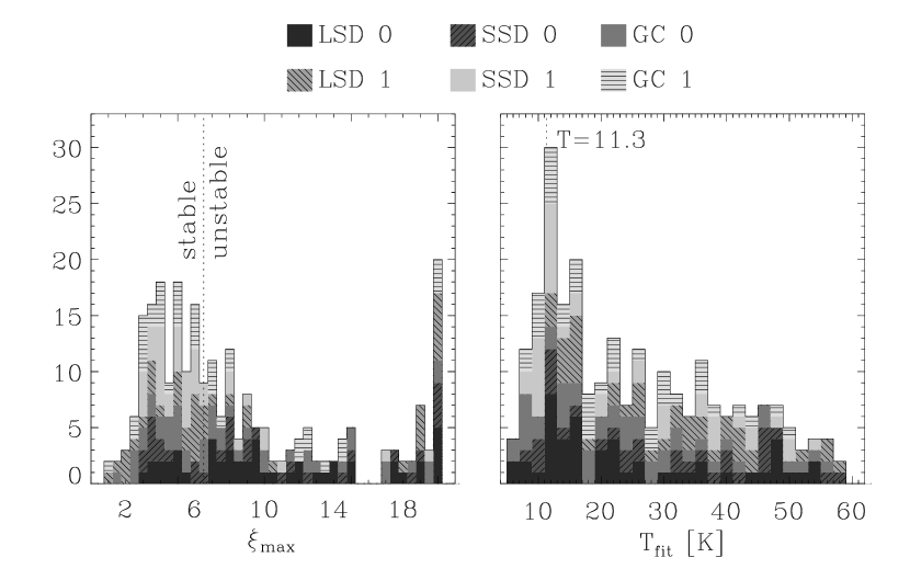
Figure 4: Histograms of (a) $\xi_{\rm max}$, and (b) $T_{\rm fit}$. The contribution of the different models are denoted by the different grayscale tone. Regarding $\xi_{\rm max}$, note that approximately 1/2 of the cores exhibit a stable BE profile (47.15%). Regarding the temperature, the distribution is broad, ranging from 5 to 60. Note also that the simulations are isothermal, implying that the fitted temperature can not correspond to the actual temperature of the core.

In Fig.’s 4a and b, we show the distribution of the fit parameters $\xi_{\rm max}$, and $T_{\rm fit}$. The contribution of each one of the six physical situations is represented with a different gray-scale tone. In the first histogram, the vertical dotted line at $\xi_{\rm max}$ $=$ 6.5 denotes the critical value above which a BE density profile corresponds to an unstable equilibrium. We note that roughly half (47.2%) of the fits have $\xi_{\rm max}$$\leq 6.5$, making the cores to appear as stable configurations. In Fig. 4b the histogram exhibits a broad distribution of fit temperatures, ranging between 5 K and 60 K, although most of them have temperatures between 5 and 30 K. Recall that the numerical simulations are isothermal, with the scaling taken such that $T=11.3$ K. Thus, we see that the temperature derived from the BE fit procedure does not recover the actual temperature of the core very well. Finally, in Fig. 4c (right), we show that most of the fits extend to radii $R_{\rm core}$ between 0.04 and 0.1 pc, but there are several cores whose BE density distributions extend up to $\sim 0.13$ pc. These values are similar to the values of the BE fits shown in the literature (Shirley et al., 2000; Johnstone et al., 2000; Alves et al., 2001; Evans et al., 2001; Langer & Willacy, 2001; Harvey et al., 2001).

An important remark is that, amongst the 248 accepted fits, 195 come from 65 cores that can be fit in all three directions ($x$-$y$, $x$-$z$, and $y$-$z$) simultaneously. Out of the remaining fits, 40 come from 20 cores that are fitted in only two of their three projections, and 11 cores resemble BE spheres in only one projection. Furthermore, cores that are accepted in more than one projection do not generally yield the same values for $T_{\rm fit}$, and/or $\xi_{\rm max}$. This fact is shown in Fig. 5, where we give the values obtained for the temperatures (upper 3 panels) and dimensionless radii of the BE sphere, $\xi_{\rm max}$ (lower 3 panels). Under the light of these results, the usefulness of BE-type fits to molecular cloud cores is seen to be suspect. We discuss this issue further in §5.

4.2 Column density profiles and projection effects

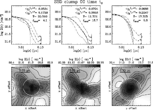
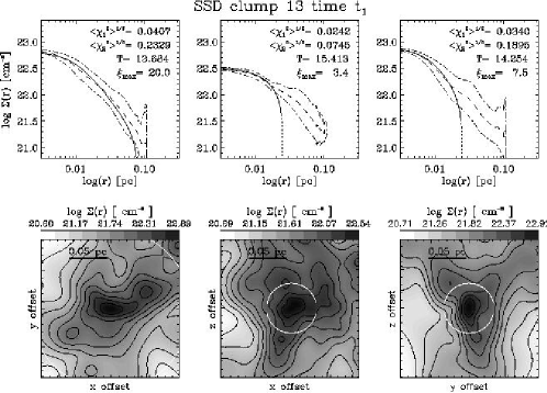
Figure 6: Column density maps and radial profiles for SSD at $t_{0}$ (a) and SSD at $t_{1}$(b). The white circles show in each case the size of $R_{\rm core}$, the radius used in the BE fit. Note the different morphologies that the same core shows in each projection.

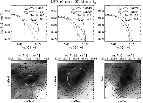
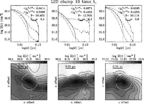
Figure 7: Similar to Fig. 6, but for LSD at $t_{0}$ (a) and $t_{1}$ (b).

We now turn to the column density structure of the cores and to the confusion that may arise due to projection effects. In Figures 6 – 8 we show column density maps and radial profiles of the six cores listed in Table 2. Upper panels show the logarithmic column density profiles, and lower panels show the column density maps in logarithmic gray-scale. In the first, the dashed line corresponds to the actual averaged density profile, dotted lines are the average $\pm$ the standard deviation column density profiles (the “dispersion” profiles), and the solid line denotes the column density of the fitted BE profile. The left, middle, and right panels respectively depict the $x$-$y$, $x$-$z$, and $y$-$z$ projections respectively. The white circle in the lower panels shows the size of the BE sphere fitted. The first point to notice is that the column density distribution within these circles is far from circularly symmetric. Instead, it is highly irregular, often elongated, and sometimes contains more than one local maximum. Nevertheless, radial profiles frequently appear soft and monotonically decreasing.

In Figs. 6a and 6b we show the maps and profiles for clump 0 in SSD at $t_{0}$ and clump 13 in SSD at $t_{1}$, respectively. For each of the three projections of the first case we fit a BE sphere with relatively good confidence at $R_{\rm core}$$=$ 0.03, 0.08 and 0.04 pc. We notice that this core has very different values of $\xi_{\rm max}$($=$ 4.1, 18.7, and 9), and of the estimated temperature $T_{\rm core}$($=$ 20.59, 11.73, and 17.73 K) for each of the projections. In the case of SSD at $t_{1}$, the values obtained using $R_{\rm core}$$=0.08$, 0.025, and 0.025 pc are $\xi_{\rm max}$$=$ 20, 3.4, and 7.5; and $T=$ 13.68, 15.41, and 14.25 K. In particular, note that in the case of SSD at $t_{1}$, the three values for $\xi_{\rm max}$ are such that the BE fit will imply unstable, stable, and unstable (but closer to critical) configurations for the $x$-$y$, $x$-$z$, and $y$-$z$ projections, respectively.

Regarding run LSD, we analyze clump 5 at $t=t_{0}$, and clump 19 at $t=t_{1}$. For the former (Fig. 7a), we find again different BE configurations for each projection; in the $x$-$y$ and $x$-$z$ projections we obtain very small values of $\xi_{\rm max}$(3.3 and 4.1 respectively, implying a core in stable equilibrium), and the core is fitted up to only 0.02 and 0.04 pc respectively, while in the $y$-$z$ projection we find $\xi_{\rm max}$ = 8.4, and the fit can be made out to 0.08 pc. The fitted temperatures for this core are 24.47, 21.13, and 25.17 K. The profiles and the maps for clump 19 in LSD at $t_{1}$ are shown in Fig. 7b. This core exhibits an elongated structure in each projection. The fitted values of $\xi_{\rm max}$  are 8.4, 15.1, and 9.6, respectively. The temperatures in each projection are more scattered than in the previous examples, being $T=25.95$, 10.71, and 33.12. It is convenient to mention that this core appears in this figure not because of the great quality of its fit, but to stress the problem of column density maps. For instance, while the maximum of the column density is located close to the maximum of the volumetric density for the $x$-$y$ and $y$-$z$ projections, the maximum column density of the $x$-$z$ projection is located almost at the edge of the box. In fact, we have found that frequently, the position of the maximum column density is shifted by several pixels from the position of the maximum volumetric density (1 pixel $=$ 0.0012 pc for LSD and SSD, and 0.0014 pc for GC), the $x$-$z$ projection being the most critical case.

Finally, we show cores 4 and 26 for run GC at $t_{0}$ and $t_{1}$ respectively. In this run, cores tend in general to be more roundish than in the other cases and thus have smaller error. Figure 8a illustrates the effects of projection. The $x$-$z$ projection (middle panel) shows a well-defined, round core, and is very well fitted by a BE sphere with $\xi_{\rm max}$ $=$ 5.1. Nevertheless, this core is just the overlap of two cores seen in projection, as shown by the $x$-$y$ and $y$-$z$ projections. A similar case is presented for GC at $t=t_{1}$ in Fig. 8b, where the $x$-$y$ projection gives an unstable fit ($\xi_{\rm max}$=8.6), while the other two projections give stable configurations (5.7 and 2.7 for the $x$-$z$ and $y$-$z$, respectively).

Before ending this section, there are some points worth noting. First of all, our criterion for a “good” fit is that $\langle\chi_{2}^{2}\rangle^{1/2}>\langle\chi_{1}^{2}\rangle^{1/2}$ (see §4.1). The algorithm was constructed to find the maximum column density in the box, which some times is shifted from the center of the box. This is because, even if the maximum volumetric density is well-centered, there is no guarantee that the column density may will be located at the same place. In particular, there are some cores that fall at the edge of the box (as mentioned before, Fig. 7b, projection $x$-$z$), and others for which $R_{\rm core}$ goes out of the box boundaries (Fig.’s 6a projection $x$-$z$, 6b projection $x$-$y$, and 7a projection $y$-$z$). In these cases, the radial profile was computed by considering only the density structure inside the box.

4.3 The physical conditions in the clumps

Throughout this paper, we have repeatedly stated that the cores and clumps in the simulations are not hydrostatic, but are instead dynamic, transient entities. This is obviously the case of the cores selected at $t_{0}$ in runs LSD and SSD, since self gravity has not been turned on at this stage yet. So, the fact that we have many acceptable fits at this time is a clear proof that BE fits to the cores’ column density profiles do not provide unambiguous evidence of the cores being in hydrostatic equilibrium.

It is moreover instructive to analyze the cores’ physical structure, and compare it to the observational data. A detailed study of the clump evolution and a comparison between the kinematics and line profiles of the simulations and the observations will be presented in a future contribution. Nevertheless, here we wish to give just a brief discussion of the the density and velocity profiles along the three coordinate axes for each one of the six cores presented in the previous section, in order to show their similarity with observed cores, and further justify our claim of non-hydrostatic conditions within them.

Figure 9 shows density (solid lines) and velocity (dotted lines) cuts for the clumps presented in Fig. 6 (clumps 0 at $t_{0}$ and 13 at $t_{1}$); Fig. 10 shows similar cuts for the clumps presented in Fig. 7 (clumps 5 at $t_{0}$ and 19 at $t_{1}$); and Fig. 11 shows cuts for clumps 4 at $t_{0}$ and 26 at $t_{1}$, presented in Fig. 8. Thin lines denote $x$ axis cuts of the density (solid) and the $x$-component of the velocity field ($v_{x}$, dotted). Similarly, intermediate bold lines denote cuts along the $y$ axis of the density and $v_{y}$, while thick lines denote $z$-axis cuts of the density and $v_{z}$. From these figures, various points are worth noting. First, the density profiles are asymmetrical at least in one of the projections. Second, the velocity profile across the clump exhibits, at least in one of the three cuts, a difference larger than the sound speed (=0.1, in code units). Third, the velocity gradients exhibited by the cores show that, (a) in the SSD cores (Fig. 9), there are some directions of contraction (negative gradients of the velocity), and some directions of expansion (positive gradients). (b) The same occurs for clump 19 at $t_{1}$ in LSD, but in the case of clump 5 at $t_{0}$ for LSD, the three directions show positive gradients of the velocity field, suggesting that this clump is actually re-expanding. (c) The cores in GC always show negative gradients, a natural result because these runs are not turbulent, and gravitational contraction is the only possible mechanism to form condensations.

The shapes and amplitudes of the velocity profiles across the clumps show that they are qualitatively similar to observed cores, in the following senses: a) The simulated clumps are transonic, exhibiting both sub- and super-sonic velocity differences across them, similarly to the reported velocity dispersions for observed cores (see, e.g., Jijina, Myers, & Adams, 1999). b) The velocity patterns include both inflow and outflow, which also occurs in real cores when observed at high enough resolution (Myers, Evans & Ohashi 2000, and references therein). Thus, our dynamic cores are not dissimilar to observed molecular cloud cores. Nevertheless, observation of the evolution of the simulations clearly shows that the cores are not hydrostatic structures, having typical lifetimes of the order of their crossing times (Kleesen & Lin 2003; see also Vázquez-Semadeni et al. 1996).

5 Summary and Discussion

5.1 Bonnor-Ebert fits

We have analyzed cores in SPH simulations of molecular clouds from Klessen et al. (1998), Klessen & Burkert (2000, 2001) and Klessen et al. (2000). The advantage of using SPH simulations over, for example, a regular fixed-grid Eulerian code, is that in the SPH case, density enhancements are better resolved spatially, allowing us to make a detailed study of cores at scales between 3$\times$10^-3 pc and 0.3 pc, the relevant scales for molecular cloud cores.

We have found cores whose angle-averaged column density profiles are well fitted by BE profiles in a variety of physical situations: with and without self-gravity (respectively, times $t_{1}$ and $t_{0}$), with turbulent driving at large and small scales (respectively LSD and SSD), and even cases with merely random, Gaussian initial density fluctuations (case GC). Several results are found. First, we have shown that 65% of the column density profiles studied may resemble BE profiles, in spite of the fact that the cores are not in hydrostatic equilibrium, and the fact that at $t=t_{0}$ the self-gravity has not been included yet for the turbulent runs LSD and SSD.

Second, we have found that BE fits give temperature values in a range between 5 and 60 K, with most of them being between 5 and 30 K. The fitted central densities range between $\sim$ 10⁴ cm^-3 and $\sim$ 10⁷ cm^-3, with most of them between 2$\times$10⁵ cm^-3 and 10⁶ cm^-3. These values are similar to the values found in the literature (Shirley et al., 2000; Johnstone et al., 2000; Alves et al., 2001; Evans et al., 2001; Langer & Willacy, 2001; Harvey et al., 2001). Nevertheless, the fitted values of the temperature and density in general do not represent the values for the actual cores. Specifically, the actual temperature of the cores is always 11.3 K, while the fitted value of the density is typically smaller than the actual density. The values of the non-dimensional radius $\xi_{\rm max}$ range between 2 and 20, with 47% of them below 6.5, and would seem to suggest that an important fraction of the fitted cores are in hydrostatic equilibrium, while in reality they are transient objects.

5.2 Goodness of fit, and the stability of B68

A natural question refers to the goodness of our fits. We have proposed that two conditions must be satisfied in order for us to accept a fit. First, the core under consideration should not contain a collapsed object, i.e. it should not yet have formed a sink particle in our numerical scheme, as we are not able to resolve such object. Second, the rms separation between the fitted and the angle-averaged (“mean”) column density profiles must be smaller than the rms separation between the dispersion profile and the mean profile. These two conditions are met in about 1/2 of the analyzed cores. The typical dispersion curves of the fits for the accepted cores are not significantly different from the error bars of several observational studies (Shirley et al., 2000; Johnstone et al., 2000; Alves et al., 2001; Evans et al., 2001; Langer & Willacy, 2001; Harvey et al., 2001) and, like in those studies, our fits generally span one to two orders of magnitude in column density. One notable exception is the fit of Bok globule B68 by Alves et al. (2001), which has remarkably small error bars. In that work, the column density map is defined over $\sim 1000$ positions (the positions of the background stars), which corresponds to an equivalent resolution of $\sqrt{1000}\sim 30$ pixels per dimension on the plane of the sky. The reported error bar at each radius in that paper is calculated as the standard deviation of the observational uncertainties of all positions at such radius (J. Alves, private communication). In fact, those authors comment that their column density profile is the highest signal-to-noise radial column density profile ever obtained for Barnard 68. For comparison, in our simulations we know the value of the column density without uncertainty over more than $128^{2}=16,384$ positions on the projection plane, but our rms errors are nevertheless larger, except for some cases in the GC runs. This appears to suggest that B68 may actually be an especially smooth and roundish structure, at least as seen from Earth. Although this is consistent with the fact that B68 is actually located within an H II region, and so the BE paradigm of thermal pressure confinement by a hotter, more tenuous medium, is applicable in this case, there are still some pieces of inconsistency concerning this core: First, the core is not round, or elliptical. This makes it implausible that it can be in precise hydrostatic equilibrium. Second, their recently reported observations show motions of 0.25$-$0.5 the sound speed, suggesting that the cloud is near but not precisely in hydrostatic equilibrium. And third, the fitted Bonnor-Ebert profile by Alves et al. (2001) implies a temperature of 16 K, and, even at this temperature, marginal instability. The actual temperature is $\sim 10$ K, i.e., a factor of 30-50% lower that that (Hotzel, Harju, & Juvela, 2002), and thus the thermal support is even lower. Thus, even within the context of BE spheres, this core is unstable by a wide margin, and therefore the hydrostatic model does not appear to provide a satisfactory explanation of its physical state. In the next section we suggest a possible alternative for B68.

5.3 Projection effects

We have shown that the cores in the simulations are in general far from spherical, similarly to the situation for actual molecular cloud cores, and that they may exhibit substantially different column density profiles, depending on the projection direction. Cores often exhibit different morphologies in different directions, and the radius at which they seem to merge with their surroundings is not unique, also depending on the direction of the projection. The projection effects play an important role here, and a core apparently well-defined in one projection may appear as a highly structured column density profile in the others. An extreme case is presented by Boss & Hartmann (2001), who show that a reasonable Bonnor-Ebert fit can be obtained even to a disk-like structure seen edge-on.

In this regard it is important to mention that, in order to minimize confusion of cores that are in the same line of sight (LOS) but whose separation is large enough to be considered dynamically disconnected from each other (as was often the case in the structures analyzed by Ballesteros-Paredes et al. 1999; Ballesteros-Paredes & Mac Low 2002), we have chosen sub-boxes of size one-tenth of the full computational domain. Thus, the sub-boxes have sizes of 0.154 pc in the SSD and LSD cases, and of 0.18 pc in the GC case, around the center of the three-dimensional core, and the LOS integration for producing the column density maps was performed only over the length of these sub-boxes. Since, even within these small length scales there is substantial substructure in the simulations, it is reasonable to expect that observed regions of comparable size in molecular clouds should also contain significant amounts of substructure, the apparent observational smoothness of some cores possibly being the result of LOS crowding, as occurs for example in Fig. 8.

The possibility that there is substructure at such small scales is consistent with the fact that most newborn stars belong to multiple systems and thus they must be born in structured, non-uniform cores. Observational evidence that molecular cores at these scales can have substantial clumpy structure is given by Velusamy, Kuiper & Langer (1995) and Wilner et al. (2000), who show that B335, recognized earlier as one of the best candidates of an isolated, round globule in a collapsing phase (see Myers, et al. 2000, and references therein), exhibits a complex, asymmetrical structure, and where the physical conditions of the infalling gas suggest that the standard model of protostellar collapse fails.

This possibility, together with inspection of Fig. 8, suggests an interesting alternative for the nature of B68. In this figure, we show one sub-box that has an exceptionally good BE fit on the $x$-$z$ projection plane, while on the other two projection planes it is seen to consist of two density peaks. Thus, the goodness of the BE fit to B68 by Alves et al. (2001) is not an unambiguous proof of the core’s BE-like nature, even though, for this particular core, this is not unlikely either.

We conclude that the evidence based on the BE fitting procedure that cores in molecular clouds are in hydrostatic equilibrium is inconclusive. In order to discriminate between the standard picture of low-mass star formation that proposes that cores are quiescent and the turbulent picture that states that they are dynamical, transient entities, we need more detailed observations and theoretical work, although we emphasize that, to date, there is no numerical model which allows for a turbulent molecular cloud that has produced quiescent cores, while the cores analyzed here do show similar physical conditions to those typically reported for real cores.

Figure 1: Ratio of $\langle\chi_{1}^{2}\rangle^{1/2}/\langle\chi_{2}^{2}\rangle^{1/2}$ vs. $\langle\chi_{1}^{2}\rangle^{1/2}$ for the cores with good BE fit. Since the rms distance between a good fit and the actual profile must be smaller than the rms distance between the dispersion curve and the actual profile, the points fall below the dotted line.

Figure 2: Number of cores with good BE fit. LSD is represented by the first two columns. SSD is represented by the middle two, and GC is represented by the last two columns. Dotted lines at 45 degrees represent cores at $t=t_{0}$, and solid lines at -45 degrees represent cores evaluated at $t=t_{1}$.

Figure 3: Ratio $n_{\rm 0\ core}$/$n_{\rm 0\ fit}$ as a function of $n_{\rm 0\ core}$. Note that there is a tendency of $n_{\rm 0\ fit}$to be smaller than $n_{\rm 0\ core}$, but no a clear trend is found regarding the time under analysis.

Figure 5: Scatter plots of temperature (upper panels), and $\xi_{\rm max}$(lower panels). Left column shows $x$-$z$ against $x$-$y$ projections. Middle column shows $y$-$z$ against $x$-$z$ projections, and right column shows $y$-$z$ against $x$-$y$ projections. Note that if all the projections had consistent BE profiles, the points should fall along the identity line in each plot. The square areas in the lower left corner of lower panels indicate the regime of nominally stable cores.

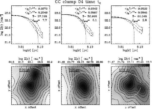
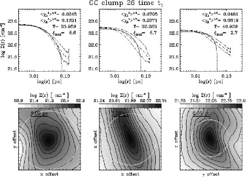
Figure 8: Similar to Fig. 6, but for GC at $t_{0}$ (a) and $t_{1}$ (b).

Figure 9: Density (solid lines, left $y$ axis) and velocity (dotted lines, right $y$ axis) cuts for clumps in Fig. 6 (SSD), in physical units (sound speed $c=0.2$ km s^-1). Left panel shows the profiles for clump 0 at $t_{0}$, and right panel shows the profiles for clump 13 at $t_{1}$. Thin lines represent cuts along the $x$ axis, intermediate bold lines represent cuts along the $y$ axis, and thick lines represent cuts along the $z$ axis. See §4.3. Note that the profiles go through the position of the volumetric density maximum, which does not necessarily correspond to the position of the column density maximum (center of the white circle in Fig. 6).

Figure 10: Similar to Fig. 9, but for clumps in Fig. 7 (LSD).

Figure 11: Similar to Fig. 9, but for clumps in Fig. 8 (GC).

Table 1: Model properties.

Run	Timea	Turbulence	$\ell_{\rm drv}^{b}$	$M_{\rm rms}^{c}$	$L_{\rm box}^{d}$	$\langle n({\rm H}_{2})\rangle^{e}$	$c_{\rm s}^{f}$	Referenceg
	[$10^{5}\,$y]		[pc]		[pc]	[cm-3]	[km s-1]
SSD	0	small-scale driven	0.19	10	1.54	$3.3\times 10^{3}$	0.2	${\cal B}3h$ in KHM00h
SSD	30.6	small-scale driven	0.19	10	1.54	$3.3\times 10^{3}$	0.2	${\cal B}3h$ in KHM00g
LSD	0	large-scale driven	0.77	10	1.54	$3.3\times 10^{3}$	0.2	${\cal B}1h$ in KHM00
LSD	2.3	large-scale driven	0.77	10	1.54	$3.3\times 10^{3}$	0.2	${\cal B}1h$ in KHM00
GC	3.1	none	—	—	1.8	$3.3\times 10^{3}$	0.2	${\cal I}1h$ in KB00
GC	6.5	none	—	—	1.8	$3.3\times 10^{3}$	0.2	${\cal I}1h$ in KB00

Table 2: Properties of cores.

Run	Time	Core #	Projection	$n_{core}$	$n_{\rm fit}$	$T_{\rm fit}$	$\xi_{\rm max}$	$R_{\rm core}$	$\chi_{1}^{2}$	$\chi_{2}^{2}$
				[cm-3]	[cm-3]	K		[pc]
SSD	$t_{0}$	00	x-y	4.24$\times$105	7.07$\times$105	20.59	4.1	0.03	0.053	0.174
			x-z	6.36$\times$105	7.07$\times$105	11.73	18.7	0.08	0.070	0.385
			y-z	7.07$\times$105	7.07$\times$105	17.73	9.0	0.04	0.069	0.225
SSD	$t_{1}$	13	x-y	9.43$\times$105	7.86$\times$105	13.68	20.0	0.08	0.041	0.233
			x-z	3.14$\times$105	7.86$\times$105	15.41	3.4	0.025	0.024	0.07
			y-z	1.49$\times$106	7.86$\times$105	14.25	7.5	0.025	0.035	0.190
LSD	$t_{0}$	05	x-y	6.73$\times$105	6.12$\times$105	24.47	3.3	0.02	0.020	0.109
			x-z	1.84$\times$105	6.12$\times$105	21.13	4.1	0.04	0.055	0.270
			y-z	3.06$\times$105	6.12$\times$105	25.17	8.4	0.08	0.027	0.300
LSD	$t_{1}$	19	x-y	2.24$\times$106	3.74$\times$106	25.95	8.4	0.03	0.041	0.339
			x-z	2.99$\times$106	3.74$\times$106	10.71	15.1	0.03	0.087	0.423
			y-z	3.74$\times$106	3.74$\times$106	33.12	9.6	0.03	0.030	0.421
GC	$t_{0}$	04	x-y	3.77$\times$105	4.19$\times$105	37.20	7.7	0.08	0.027	0.205
			x-z	4.19$\times$105	4.19$\times$105	53.0	5.1	0.06	0.034	0.099
			y-z	2.10$\times$105	4.19$\times$105	61.05	2.8	0.05	0.052	0.085
GC	$t_{1}$	26	x-y	4.30$\times$105	3.91$\times$105	33.96	8.6	0.08	0.025	0.133
			x-z	2.34$\times$105	3.91$\times$105	32.28	5.7	0.07	0.071	0.207
			y-z	1.56$\times$105	3.91$\times$105	48.94	2.7	0.05	0.048	0.082

References

- Alves et al. (2001) Alves, J., Lada, C. J., & Lada, E. A. 2001, Nature, 409, 159
- Andre, Ward-Thompson & Barsony (2000) Andre, P., Ward-Thompson, D., & Barsony, M. 2000. Protostars and Planets IV, ed, V. Mannings, A. Boss, & S. Russell (Tucson:Univ. Arizona Press), 59
- Ballesteros-Paredes & Mac Low (2002) Ballesteros-Paredes, J. & Mac Low, M.-M. 2002, ApJ, 570, 734
- Ballesteros-Paredes et al. (1999a) Ballesteros-Paredes, J., Hartmann, L., & Vázquez-Semadeni, E. 1999a, ApJ, 527, 285
- Ballesteros-Paredes et al. (1999b) Ballesteros-Paredes, J., Vázquez-Semadeni, E., & Scalo, J. 1999b, ApJ, 515, 286
- Bate, Bonnell & Price (1995) Bate, M. R., Bonell, I. ., & Price, N. M. 1995. MNRAS, 277, 362
- Benz (1990) Benz, W. 1990, in The Numerical Modelling of Nonlinear Stellar Pulsations, ed. J. R. Buchler, p. 269, Kluwer Academic Publishers, The Netherlands
- Bonnor (1956) Bonnor, W. B. 1956, MNRAS, 116, 351
- Boss & Hartmann (2001) Boss, A. P. & Hartmann, L. W. 2001, ApJ, 562, 842
- Bourke et al. (2001) Bourke, T. L., Myers, P. C., Robinson, G., & Hyland, A. R. 2001, ApJ, 554, 916
- Chandrasekhar (1939) Chandrasekhar, S. 1939. An introduction to the study of stellar structure. The University of Chicago press
- Chappell & Scalo (2001) Chappell, D. & Scalo, J. 2001, ApJ, 551, 712
- Crutcher (1999) Crutcher, R. M. 1999, ApJ, 520, 706
- Ebert (1955) Ebert, R. 1955, Zeitschrift für Astrophysik, 36, 222
- Evans et al. (2001) Evans, N. J., Rawlings, J. M. C., Shirley, Y. L., & Mundy, L. G. 2001, ApJ, 557, 193
- Falgarone, Phillips & Walker (1991) Falgarone, E., Phillips, T. G., & Walker, C. K. 1991, ApJ, 378, 186
- Goldsmith & Langer (1978) Goldsmith, P. F. & Langer, W. D. 1978, ApJ, 222, 881
- Goldsmith (1988) Goldsmith, P. F. 1988, Molecular Clouds, MilkY-Way and External Galaxies, 1
- Hartmann et al. (2001) Hartmann, L., Ballesteros-Paredes, J., & Bergin, E. A. 2001, ApJ, 562, 852
- Harvey et al. (2001) Harvey, D. W. A., Wilner, D. J., Lada, C. J., Myers, P. C., Alves, J. ;., & Chen, H. 2001, ApJ, 563, 903
- Heitsch, Mac Low & Klessen (2001) Heitsch, F., Mac Low, M.-M., & Klessen, R. S. 2001, ApJ, 547, 280
- Hotzel, Harju, & Juvela (2002) Hotzel, S., Harju, J., & Juvela, M. 2002, A&A, 395, L5
- Houlahan & Scalo (1990) Houlahan, P. & Scalo, J. 1990, ApJS, 72, 133
- Houlahan & Scalo (1992) Houlahan, P. & Scalo, J. 1992, ApJ, 393, 172
- Jijina, Myers, & Adams (1999) Jijina, J., Myers, P. C., & Adams, F. C. 1999, ApJS 125, 161
- Johnstone et al. (2000) Johnstone, D., Wilson, C. D., Moriarty-Schieven, G., Joncas, G., Smith, G., Gregersen, E., & Fich, M. 2000, ApJ, 545, 327
- Klessen (2001) Klessen, R. S. 2001, ApJ, 556, 837
- Klessen & Burkert (2000) Klessen, R. S. & Burkert, A. 2000, ApJS, 128, 287
- Klessen & Burkert (2001) Klessen, R. S. & Burkert, A. 2001, ApJ, 549, 386
- Klessen et al. (1998) Klessen, R. S., Burkert, A., Bate, M. R. 1998, ApJ, 501, L205
- Klessen et al. (2000) Klessen, R. S., Heitsch, F., & Mac Low, M.-M., 2000, ApJ, 535, 887
- Klessen & Lin (2003) Kleesen, R. S. & Lin, D.N.C. 2003. Physical Review E, in press
- Langer & Willacy (2001) Langer, W. D. & Willacy, K. 2001, ApJ, 557, 714
- Lee & Myers (1999) Lee, C. W. & Myers, P. C. 1999, ApJS, 123, 233
- Léorat, Passot & Pouquet (1990) Léorat, J., Passot, T., & Pouquet, A. 1990, MNRAS, 243, 293
- Mac Low & Klessen (2003) Mac Low, M.-M. & Klessen, R. S. 2003, Rev. Mod. Phys., submitted (Astro-ph/0301093)
- Mac Low & Ossenkopf (2000) Mac Low, M.-M. & Ossenkopf, V. 2000, A&A, 353, 339
- Mac Low et al. (1998) Mac Low, M.-M., Klessen, R. S., Burkert, A., & Smith, M. D. 1998, Phys. Rev. Lett., 80, 275
- Monaghan (1992) Monaghan, J. J. 1992, ARA&A, 30, 543
- Myers, Evans & Ohashi (2000) Myers, P. C., Evans, N. J., & Ohashi, N. 2000, Protostars and Planets IV, 217
- Nakano (1998) Nakano, T. 1998, ApJ, 494, 587
- Ostriker et al. (1999) Ostriker, E. C., Gammie, C. F., & Stone, J. M. 1999, ApJ, 513, 259
- Padoan & Nordlund (1999) Padoan, P. & Nordlund, Åke 1999, ApJ, 526, 279
- Scalo (1985) Scalo, J. M. 1985, Protostars and Planets II, ed. D.C. Black & M.S. Mattheus (Tucson:Univ. Arizona Press), 201
- Shirley et al. (2000) Shirley, Y. L., Evans, N. J., Rawlings, J. M. C., & Gregersen, E. M. 2000, ApJS, 131, 249
- Shu et al. (1987) Shu, F. H., Adams, F. C., & Lizano, S. 1987, ARA&A, 25, 23
- Scalo et al. (1998) Scalo, J., Vázquez-Semadeni, E., Chappell, D., & Passot, T., 1998, ApJ, 504, 835
- Spaans & Silk (2000) Spaans, M. & Silk, J., 2000, ApJ, 538, 115
- Stone, Ostriker & Gammie (1998) Stone, J. M., Ostriker, E. C., & Gammie, C. F. 1998, ApJ, 508, L99
- Tafalla et al. (2002) Tafalla, M.; Myers, P.C.; Caselli, P., & Walmsley, C.M. 2002. ApJ in press.
- Taylor et al. (1996) Taylor, S. D., Morata, O., & Williams, D. A. 1996, A&A, 313, 269
- Tohline, Bodenheimer & Christodoulou (1987) Tohline, J. E., Bodenheimer, P. H., & Christodoulou, D. M. 1987, ApJ, 322, 787
- Vázquez-Semadeni (1994) Vázquez-Semadeni, E. 1994, ApJ, 423, 681
- Vázquez-Semadeni et al. (2003a) Vázquez-Semadeni, Ballesteros-Paredes & Klessen, 2003. ApJ, in press
- Vázquez-Semadeni et al. (2000) Vázquez-Semadeni, E., Ostriker, E. C., Passot, T., Gammie, C. F., & Stone, J. M. 2000, Protostars and Planets IV, ed. V. Mannings, A. Boss & S. Russell (Tucson:Univ. Arizona Press), 3
- Vázquez-Semadeni et al. (1996) Vázquez-Semadeni, E., Passot, T., & Pouquet, A. 1996, ApJ, 473, 881
- Vázquez-Semadeni et al. (2003b) Vázquez-Semadeni, E., Shadmeri, M., & Ballesteros-Paredes, J. 2002b. ApJ, submitted
- Velusamy, Kuiper & Langer (1995) Velusamy, T., Kuiper, T. B. H., & Langer, W. D. 1995, ApJ, 451, L75
- Visser, Richer & Chandler (2002) Visser, A. E., Richer, J. S., & Chandler, C. J. 2002. AJ, in press
- Williams, Blitz & McKee (2000) Williams, J. P., Blitz, L., & McKee, C. F. 2000, Protostars and Planets IV, ed. V. Mannings, A. Boss & S. Russell (Tucson:Univ. Arizona Press), 97
- Wilner et al. (2000) Wilner, D. J., Myers, P. C., Mardones, D., & Tafalla, M. 2000, ApJ, 544, L69