The Galaxy Angular Correlation Functions and Power Spectrum from the Two Micron All Sky Survey

Abstract

We calculate the angular correlation function of galaxies in the Two Micron All Sky Survey. We minimize the possible contamination by stars, dust, seeing and sky brightness by studying their cross correlation with galaxy density, and limiting the galaxy sample accordingly. We measure the correlation function at scales between $1\arcmin<\theta<18\arcdeg$ using a half million galaxies. We find a best fit power law to the correlation function has a slope of $-0.79\pm 0.02$ and an amplitude at $1\arcdeg$ of $0.10\pm 0.01$ in the range $1\arcmin-2.5\arcdeg$. However, there are statistically significant oscillations around this power law. The largest oscillation occurs at about 0.8 degrees, corresponding to $700h^{-1}$ kpc at the median redshift of our survey, as expected in halo occupation distribution descriptions of galaxy clustering. In addition, there is a break in the power-law shape of the correlation function at $\theta>2.5\arcdeg$. Our results are in good agreement with other measurements of the angular correlation function.

We invert the angular correlation function using Singular Value Decomposition to measure the three-dimensional power spectrum and find that it too is in good agreement with previous measurements. A dip seen in the power spectrum at small wavenumber $k$ is statistically consistent with CDM-type power spectra. A fit of CDM-type power spectra in the linear regime ($k<0.15h$ Mpc^-1) give constraints of $\Omega_{m}h=0.13\pm 0.07$ and $\sigma_{8}=1.0\pm 0.09$ for a spectral index of $1.0$. This suggest a $K_{s}$-band linear bias of $1.1\pm 0.2$. These measurements are in good agreement with other measurements of the power spectrum on linear scales. On small scales the power-law shape of our power spectrum is shallower than that derived for the Sloan Digital Sky Survey. This may imply a biasing for these different galaxies that could be either waveband or luminosity dependent. The power spectrum derived here in combination with the results from other surveys can be used to constrain models of galaxy formation.

1. Introduction

Correlation statistics are an important method for relating galaxies to the underlying mass distribution. The angular correlation function, $w(\theta)$, measures the projected clustering of galaxies by comparing the distribution of galaxy pairs relative to that of a random distribution. While a less direct probe than the three-dimensional correlation function $\xi(r)$, the angular correlation function can be a powerful approach owing to the larger sizes of two-dimensional surveys. The angular correlation function for bright galaxies has been measured for the Lick Survey (Groth & Peebles, 1977), the Automated Plate Measuring (APM) Galaxy Survey (Maddox et al., 1990, 1996), the Edinburgh Durham Southern (EDS) Galaxy Catalog (Collins et al., 1992), and the Muenster Red Sky Survey (Boschán, 2002). Most recently the Sloan Digital Sky Survey (SDSS; York et al., 2000) has performed a very detailed analysis of the angular correlation function (Connolly et al., 2002; Scranton et al., 2002) from their Early Data Release (EDR; Stoughton et al., 2002).

Additionally, numerous papers have been written on techniques for inverting the angular correlation function to determine the full three-dimensional power spectrum, $P(k)$ (Limber, 1953; Lucy, 1974; Baugh & Efstathiou, 1993; Dodelson & Gaztañaga, 2000; Efstathiou & Moody, 2001; Eisenstein & Zaldarriaga, 2001; Padilla & Baugh, 2003).

In this paper we calculate the angular correlation function for galaxies selected from the Two Micron All Sky Survey (2MASS; Skrutskie et al., 1997). We then invert $w(\theta)$ using Singular Value Decomposition, as suggested by Eisenstein & Zaldarriaga (2001), to measure the three-dimensional power spectrum. A preliminary analysis of $w(\theta)$ and $P(k)$ for the Second Incremental Data Release of the 2MASS catalog was performed by Allgood et al. (2001). Here we use the complete and final 2MASS catalog, which provides a more than two-fold increase in the number of sources owing to the nearly full sky ($>98\%$, Jarrett et al., 2000b) coverage, and removes the significant complication of coverage masking suffered by Allgood et al. (2001). In addition, the final 2MASS pipeline processing has improvements in the flux measurements that affect the catalog completeness.

The angular correlation function of the 2MASS galaxies is interesting for a number of reasons. First, with 2MASS we can characterize the large-scale clustering of galaxies in the near-infrared (NIR) using the $K_{s}$ (2.15µm) passband. Galaxy $K_{s}$ light is 5-10 times less sensitive to dust and stellar populations than $B$-band light, providing a more uniform survey of the galaxy population. Because the $K_{s}$-band most closely measures stellar mass, it is possible that the $K_{s}$ selected correlation function is a better probe of the dark matter power spectrum than $B$ and $R$-band selected measurements. The variations of correlation functions in different bands contain information about how galaxy properties are related to the underlying dark matter distribution and, therefore, to their formation and evolution.

Secondly, 2MASS has full sky coverage extending out to a median redshift of $z=0.07$ and, hence, measures the power spectrum of our local Universe. Knowledge of our local “cosmography”, and how it may differ from other regions of the Universe, is relevant for many cosmological tests. Thus the angular correlation function and power spectrum from 2MASS are valuable tools for understanding galaxy formation and cosmology especially when used in comparison with measurements from other surveys.

Our paper largely follows the treatment of the Sloan EDR performed by Scranton et al. (2002), Connolly et al. (2002) and Dodelson et al. (2002) and is outlined as follows: In §2 we describe our galaxy sample selection from 2MASS. In §3 we analyze the importance of systematic errors by studying their cross correlation with galaxy density. In §4 we calculate the correlation function and discuss its errors, and in §5 we invert $w(\theta)$ to measure the three-dimensional power spectrum, $P(k)$. We conclude in §6.

2. 2MASS Selected Galaxies

To measure the angular correlation function accurately, it is critically important to fully understand the reliability and completeness of the galaxy sample. We select galaxies from the 2MASS extended source catalog (XSC; Jarrett et al., 2000b), which contains over 1.1 million extended objects brighter than $K_{s}=14$ mag. The detection of galaxies is limited predominantly by confusion noise from stars, whose number density increases exponentially towards $|b|=0\arcdeg$. The XSC is mostly galaxies at $|b|>20\arcdeg$ ($>98\%$), with an increasing stellar mixture ($\sim 10\%$) at lower latitudes of $5\arcdeg<|b|<20\arcdeg$. Within the Galactic plane, i.e. $|b|<5\arcdeg$, there is an additional contamination by artifacts ($10-20\%$) and a variety of Milky Way extended sources ($\sim 40\%$) including globular and open clusters, planetary nebulae, H II regions, young stellar objects, nebulae, and giant molecular clouds (Jarrett et al., 2000a). For our final analysis, we employ a latitude cut of $|b|>20\arcdeg$ to remove the strong contamination of $w(\theta)$ from stars at lower latitudes (see §3.1). Our cut reduces the Galactic contaminant sources to $\sim 2\%$ for our galaxy sample.

The XSC also contains a fraction of spurious sources comprised of multiple star systems. Multiple star systems become an increasingly important source of contamination as the stellar density, $n_{\rm star}$ rises, where $n_{\rm star}$ is the number of $K_{s}<14$ mag stars per sq. degree calculated in a co-add which is $8.5\arcmin\times 16\arcmin$. Specifically, the reliability of separating stars from extended sources drops rapidly from $95\%$ at $|b|=10\arcdeg$ ($n_{\rm star}\approx 5,000\,{\rm deg}^{-2}$), to $<65\%$ at $|b|<5\arcdeg$ ($n_{\rm star}>10^{4}\,{\rm deg}^{-2}$) (Jarrett et al., 2000a). To remove sources that are certainly unreliable, we use a cut at $n_{\rm star}<10^{4}\,{\rm deg}^{-2}$ during our initial galaxy selection from the XSC. The stellar density is this high over $5.5\%$ of the sky so our galaxy catalog only covers $94.5\%$ of the sky. At high latitudes ($|b|>20\arcdeg$, $n_{\rm star}\lesssim 1,250\,{\rm deg}^{-2}$) the catalog is $>98\%$ reliable for sources with $K_{s}<13.5$ (Jarrett et al., 2000b). The XSC contains a small fraction of artifacts, e.g. diffraction spikes, meteor streaks, infrared airglow, at all latitudes. The XSC processing removes and/or flags most artificial sources, as described fully in Jarrett et al. (2000b). We use the XSC confusion flag (cc_flag) to remove sources identified as artifacts. We also remove a small number of bright ($K_{s}<12$ mag) sources ($\sim 2000$) with dust corrected $J-K_{s}$ colors less than $0.7$ and greater than $1.4$, which were determined to be non-extragalactic extended sources (see Maller et al., 2003). Finally, selecting in the $K_{s}$-band minimizes the inclusion of false sources caused by infrared airglow.

The XSC meets the original 2MASS science requirements: greater than 90% completeness for extended sources (extragalactic and Galactic) with $K_{s}<13.5$, and free from stellar confusion for $|b|>20\arcdeg$ (Jarrett et al., 2000b). In practice, the 2MASS completeness is a measure of the fraction of extended sources of a given magnitude that are actually detected. Huchra & Mader (2000, private communication) show that the XSC is $99\%$ complete for $|b|>30\arcdeg$ sources in the range $12.0\lesssim K_{s}\lesssim 13.7$ mag, using $\log{N}$–$\log{S}$ and $V/V_{\rm max}$ tests. At magnitudes brighter than $K_{s}=11.5$, they determine that greater than $95\%$ of the known galaxies in Zwicky & Kowal (1968) are found in the XSC. Jarrett et al. (2000a) find the XSC completeness remains at $95\%$ for $K_{s}\leq 13.0$ sources well into the Galactic plane ($|b|>5\arcdeg$). Additionally, Bell et al. (2003) cross correlate the XSC with the complete ($>99\%$ Strauss et al., 2002), spectroscopic galaxy sample drawn from the SDSS EDR. Bell et al. (2003) find that in the large (414 square degree), high latitude ($|b|>30\arcdeg$) region of the EDR, the XSC misses only 2.5% of the known galaxy population down to $K_{s}<13.57$ in dust corrected Kron magnitudes.

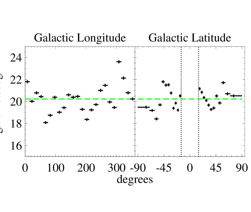
Figure 1.— The density of 2MASS galaxies on the sky in bins of Galactic longitude ($l$), and latitude ($b$). The horizontal error bars represent the width of each bin, while the Poisson uncertainties are given by vertical error bars. The dotted lines in the right-hand panel delineate the $|b|<15\arcdeg$ region corresponding to the Galactic plane. The dashed line shows the average galaxy density of $20.2$ deg^-2. There is a significant variation between regions but there is no trend with longitude or latitude.

2MASS employs Kron (1980) magnitudes to obtain the total flux of each galaxy. The 2MASS-defined Kron magnitudes (k_m_fe in the XSC) are elliptical aperture magnitudes with semi-major axes equal to 2.5 times the first moment of the brightness distributions for each source. The first moment calculation, the Kron radius, is computed to a radius that is five times the 20 mag arcsec^-2 isophote. 2MASS limits the Kron radius to a $5\arcsec$ minimum (owing to the PSF; see the 2MASS Explanatory Supplement for details). Because of the short exposure times (7.8 seconds with a 1.3-m telescope, Skrutskie et al., 1997) of 2MASS, the Kron magnitudes underestimate the true total flux systematically by approximately $0.1$ magnitudes (Bell et al., 2003). At a magnitude limit slightly fainter than the 2MASS science requirement, $K_{s}\sim 13.57$, the XSC galaxy completeness is quite good, primarily missing only low surface brightness ($1.5\%$) and distant ($1.0\%$) galaxies both of which are near the Kron $K_{s}=13.57$ limit (Bell et al., 2003). We adopt Kron magnitudes for this paper and henceforth all cited magnitudes will be Kron magnitudes. The small fraction of low surface brightness galaxies missed in the XSC confirms the expectation of Jarrett et al. (2000b). Moreover, the automated processing of the XSC produces systematically incomplete photometry for galaxies larger than $50\arcsec$ due to the typical 2MASS scan width of $8.5\arcmin$ (Jarrett et al., 2000b). We include the 2MASS Large Galaxy Atlas sample (540 galaxies identified in the XSC database with cc_flag=‘Z’) from (Jarrett et al., 2003), which has been assembled to account for most of the scan size photometric incompleteness.

We select initially all $K_{s}<14$ mag objects from the XSC with $n_{\rm star}<10^{4}\,{\rm deg}^{-2}$. We apply Galactic foreground dust corrections from Schlegel et al. (1998) to each galaxy in the $K_{s}<14$ catalog and cut at $K_{s}=13.57$ mag, resulting in $775,562$ galaxies. The dust correction increases the number of galaxies brighter than $K_{s}=13.57$ by 10%. We plot the galaxy density as a function of longitude and latitude in Figure 1, illustrating that the dust-corrected number densities are fairly uniform for $|b|>15$. Ultimately, our final sample selection includes $501,578$ galaxies with $K_{s}<13.57$ mag, $|b|>20\arcdeg$, and Galactic dust corrections less than $0.05$ magnitudes in $K_{s}$-band (as described in §3.2). We summarize these sample cuts leading to our final selection in Table 1.

$N$	$K_{s}$	$|b|(\arcdeg)$
1,295,895	$<14.0$	$>0$
775,562	$<13.57$	$>0$
688,464	$<13.57$	$>10$
618,333	$<13.57$	$>15$
548,353	$<13.57$	$>20$
480,794	$<13.57$	$>25$
501,578	$<13.57$	$>20$

Table 1Galaxy Sample Selection. The number of galaxies in our 2MASS catalog is given as a function of $K_{s}$ magnitude cut and Galactic latitude cut. See §3.

The redshifts of many 2MASS galaxies have been measured as part of other redshift surveys. Large redshift samples provide the redshift distribution $dN/dz$ of 2MASS galaxies, and allow calculations of the NIR luminosity function (Kochanek et al., 2001; Cole et al., 2001; Bell et al., 2003). For computing the three-dimensional power spectrum (see §5), we will use redshifts from the SDSS EDR (Stoughton et al., 2002) and the 2dF Galaxy Redshift Survey (2dFGRS) 100k Data Release (Colless et al., 2001).

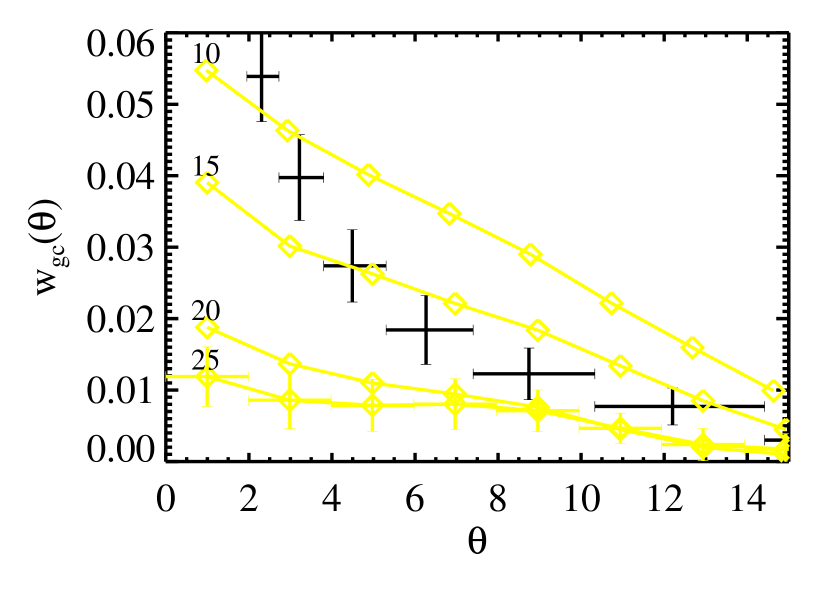
Figure 2.— Galaxy-star cross-correlations (open diamonds) for cuts in Galactic latitude of $|b|>10\arcdeg,15\arcdeg,20\arcdeg$ and $25\arcdeg$. Error bars displayed for the $25\arcdeg$ cut are representative of the other cuts. The auto-correlation is shown as naked error bars for comparison. We require a latitude cut of $|b|>20\arcdeg$ to be free of stellar contaminants out to separation angles of $\theta<15\arcdeg$.

3. Cross-Correlation Functions

Following Scranton et al. (2002, hereafter Sc02) we analyze the cross correlation between the galaxy number counts and possible sources of systematic error. This is an effective method for identifying errors, quantifying their magnitude, and determining the selection limits required to reduce them to manageable levels. Below we analyze the cross-correlation signal for four possible contaminants: stars, dust, seeing, and sky brightness.

To perform the cross correlation, we pixelize the galaxy sample on a regular grid to determine local galaxy densities. We use the HEALPix software package (G rski et al., 1999) to create equal area pixels on the sky. We use a Nside parameter of $64$ generating $N_{c}=49,152$ cells each with an area of $0.84{\rm deg}^{2}$. This yields an average of $15.6$ galaxies per cell so very few cells contain no galaxies. We calculate the average value of each contaminant for a cell using the individual measurements for each galaxy within the cell. When making a latitude cut, we include all cells whose centers are above the given latitude including galaxies that might be below the cut. To calculate errors, we subsample the data, dividing the sky into $48$ tiles, with each tile containing $1024$ cells, making them roughly $29.3\arcdeg$ on a side. Because we will perform a latitude cut and $8$ of the tiles lie along the galactic plane we will end up only using $40$ tiles for our analysis. For each tile we calculate the fractional galaxy and contaminant over density in a cell $i$ by

$$\delta^{g}_{i} = \frac{n^{g}_{i}-\bar{n}^{g}}{\bar{n}^{g}}$$ (1)

$$\delta^{c}_{i} = \frac{x^{c}_{i}-\bar{x}^{c}}{\bar{x}^{c}},$$

where the averages are calculated for each tile. The cross-correlation function, $w_{gc}(\theta)$, is then

$$w_{gc}(\theta_{\alpha})=\frac{\sum_{i,j=1}^{N_{c}}\delta^{g}_{i}\delta^{c}_{j}\Theta^{\alpha}_{ij}}{\sum_{i^{*},j^{*}=1}^{N_{c}}\Theta^{\alpha}_{i^{*}j^{*}}},$$ (2)

where $\Theta^{\alpha}_{ij}$ is unity if the separation between cells $i$ and $j$ is within angular bin $\theta_{\alpha}$ and zero otherwise. The error on the mean can be computed by

$$\left[\Delta\bar{w}_{gc}(\theta)\right]^{2}=\frac{1}{N_{t}^{2}}\sum^{N_{t}}_{i=1}\left[\bar{w}_{gc}(\theta)-w_{gc,i}(\theta)\right]^{2},$$ (3)

where $N_{t}=40$ is the total number of tiles. We use this cross-correlation function to quantify the systematic contributions of contaminants in the subsections below.

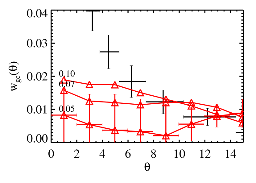
Figure 3.— Galaxy-extinction cross-correlations (open triangles) for three cuts in the maximum allowed value for the extinction given by $A(K_{s})=0.367\times E(B-V)$, with $E(B-V)$ from Schlegel et al. (1998). Error bars are shown only for the lowest cut and are representative. The auto-correlation is shown as naked error bars for comparison. A cut of $A(K_{s})\leq 0.05$ mag reduces the cross-correlation signal to less then the auto-correlation for $\theta<10\arcdeg$.

3.1. Stars

During the 2MASS pipeline processing, the stellar density $n_{\rm star}$—the number of $K_{s}<14$ mag stars per square degree—is determined for each extended source on a co-add which is $8.5\arcmin\times 16\arcmin$ in size. In regions of high stellar density, stars may be mistakenly identified as extended sources. For $95\%$ of the sky, $n_{\rm star}$ provides an excellent measure of confusion noise in the XSC. The stellar density saturates in 2MASS at values of $n_{\rm star}>3\times 10^{4}\,{\rm deg}^{-2}$ (Jarrett et al., 2000a), occurring near the Galactic center ($|b|<5\arcdeg$, $350\arcdeg<l<10\arcdeg$). Recall that for our galaxy sample we make a more conservative stellar density cut of $n_{\rm star}<10^{4}\,{\rm deg}^{-2}$.

To examine the importance of this contaminant we look at the cross-correlation of the galaxy density and the stellar density. Because $n_{\rm star}$ is a strong function of Galactic latitude we measure the cross-correlation for different Galactic latitude cuts and present the results in Figure 2. Including XSC objects with low latitudes ($|b|<15\arcdeg$) results in a higher amplitude galaxy-star cross-correlation at all angular scales than the galaxy auto-correlation. That this cross-correlation has a different slope than the galaxy auto-correlation suggests that the signal is coming from the stellar auto-correlation as multiple star systems are mistakenly identified as galaxies. However, if the latitude cut is increased to $|b|>20\arcdeg$, then the auto-correlation signal is not contaminated significantly by stars at angular separations of $\theta<15\arcdeg$. Thus, we adopt a $|b|>20\arcdeg$ cut throughout this paper. Making this cut reduces the area of the survey to $67\%$ of the sky or $28,960$ square degrees. $548,353$ galaxies survive this latitude cut.

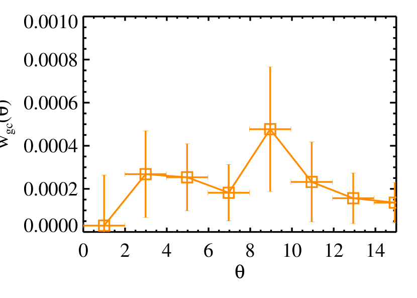
Figure 4.— The galaxy-seeing cross-correlation (open squares) as a function of angle. The auto-correlation can not be plotted because it is $>30$ times larger. Seeing variations are not a source of systematic error.

3.2. Dust

Though we have attempted to correct our galaxy sample for the effects of foreground extinction using Schlegel et al. (1998), dust may remain an important contaminant. There is a strong correlation between stellar density and dust extinction, both of which increase substantially towards the Galactic plane. Here we look at the cross-correlation between dust extinction and galaxy density only at $|b|>20\arcdeg$, owing to the stellar contamination at lower latitudes. In Figure 3, we show the galaxy-extinction cross-correlation for three cuts in magnitudes of $K_{s}$-band dust extinction. To bring the galaxy-extinction cross-correlation below the auto-correlation we mask out those cells with $K_{s}$-band extinction of $A(K_{s})=0.367\times E(B-V)>0.05$, which amounts to $2,602$ cells. This leaves and area of $23,345$ sq. degrees and $501,578$ galaxies.

Our use of a dust correction to galaxy magnitudes does increase the dust cross-correlation. For example, the amplitude of the galaxy-extinction cross-correlation is reduced by about a third for a catalog without a dust correction. However, the dust correction increases the number of galaxies by 10%, and therefore the error introduced by the correction is a minor contribution to the systematic error budget.

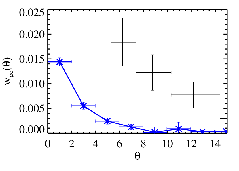
Figure 5.— The galaxy-background (Xs) cross-correlation function as a function of angle. The background error correlates with galaxy density as expected, yet it is always significantly less than the auto-correlation (naked error bars). Sky background fluctuations are a negligible source of systematic error.

3.3. Seeing

Great care has gone into ensuring that the final 2MASS release has a highly uniform seeing over the entire survey area. The pipeline processing allowed tracking of the point-spread function (PSF) as a function of time. The mean radial size of the 2MASS PSF over a scan could vary over periods as short as a few minutes. Depending on the local density of stars, the seeing was tracked on time-scales ranging from 2—30 seconds. Scans with poor seeing were reobserved under better conditions to maintain the seeing uniformity. For each source in the XSC, the pipeline measured the average radial extent of the PSF in each passband (called “ridge shape” and denoted k_sh0 in the XSC for the $K_{s}$-band), analogous to a full width at half maximum (FWHM) measurement of the varying PSF. The full details of the PSF characterization and seeing tracking are given in (Jarrett et al., 2000b).

We use k_sh0 to test for systematic errors in the angular correlation of galaxies caused by spatial variations in seeing. One might expect that observations made under poor seeing conditions would lead to more spurious galaxy detections, causing a correlation between seeing and galaxy density. For our sample the mean seeing is k_sh0 = 0.992 with 0.049 rms scatter, corresponding to a typical survey seeing of $2.1\arcsec$ FWHM with 5% uncertainty. Given this uniformity, we do not expect the seeing to be a major source of systematic errors. One might want to check for seeing variations over the scan width of $8.5\arcmin$. However, even in the densest regions there are only a few 2MASS galaxies in such a small area so a cross-correlation cannot be performed. In Figure 4 we plot the galaxy-seeing cross-correlation, whose amplitude is more than $30$ times less than the auto-correlation amplitude. Hence, seeing variations are a negligible source of systematic error.

3.4. Sky Background

In $K_{s}$-band, the dominant source of background flux is thermal continuum emission from the atmosphere. While the $K_{s}$ background is less severe and variable than the airglow induced $J$ and $H$-band backgrounds, the sky brightness at $K_{s}$ is still quite high at $13.3\pm 0.3$ mag arcsec^-2. This is orders of magnitude brighter than the typical outer isophotes of 2MASS galaxies, which have $\mu_{K}>19$ mag arcsec^-2. Furthermore, the $K_{s}$ background can be variable and may still produce high-frequency features extending to tens of arcseconds. To mitigate these features, the 2MASS processing includes a sophisticated background fitting and removal scheme that is described fully in Jarrett et al. (2000b).

The rms background error caused by Poisson noise, which depends on the variable sky brightness, might also produce sources of systematic error in calculating the angular correlation of 2MASS galaxies. The median background local to each source is determined in each passband and given in the XSC database (k_back for $K_{s}$). For each source in our sample, we estimate the background error from co-added and resampled images

$$\sigma_{\rm bkg}^{2}=\frac{k_{\rm f}^{2}}{6n_{\rm r}^{2}}\left[\frac{n_{\rm r}({\rm k\_back})}{G}+\frac{\sigma_{\rm RN}^{2}}{G^{2}}\right].$$ (4)

The factor of 6 represents the number of co-added frames comprising each source image. Each $2\arcsec$ pixel has been resampled ($n_{\rm r}=4$) into $1\arcsec$ pixels and smoothed with a kernel giving rise to the factor of $k_{\rm f}=0.5853$. In $K_{s}$-band 2MASS has an average gain of $G=8.2$ electrons/DN and an average read noise of $\sigma_{\rm RN}=52$ electrons (T. Jarrett, 2001, private communication) .

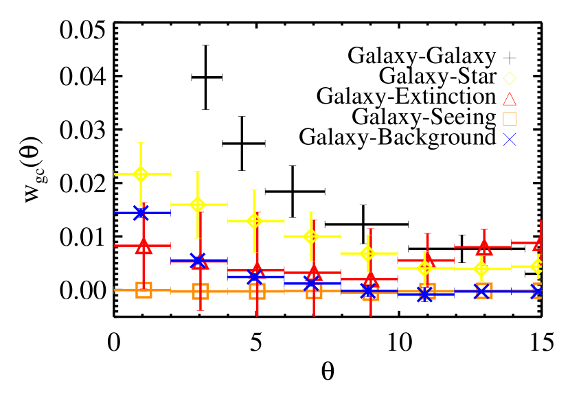
Figure 6.— The cross-correlations with all four investigated contaminants using our cuts in Galactic latitude of $b>20\arcdeg$ and in extinction of $K_{s}<0.05$ compared to the galaxy auto-correlation signal. On angular scales $<10\arcdeg$ the auto-correlation amplitude is significantly higher then the cross-correlation with any of the contaminants.

A larger sky uncertainty increases the difficulty of galaxy detection and leads to a correlation between background error and galaxy density. We find an average k_back of 475 DN with scatter 125 DN, corresponding to a background uncertainty of $20.02\pm 0.13$ mag arcsec^-2. This agrees with the typical $1\sigma$ error of 20.0 mag arcsec^-2 in $K_{s}$ (Jarrett et al., 2000b, 2003). The estimated background error is quite uniform and the galaxy density and background error correlation is weak, as we show in Figure 5. The cross-correlation amplitude is always smaller than that of the galaxy auto-correlation and hence background fluctuations are a negligible source of error in determining $w(\theta)$.

3.5. Summary of Systematic Effects

Figure 6 shows the cross-correlations of the four possible contaminants in comparison with $w(\theta)$. With the Galactic latitude cut of $|b|>20\arcdeg$ and the dust extinction cut of $K_{s}<0.05$, we see that the contaminants are significantly below the auto-correlation signal for angular scales $\theta<10\arcdeg$. We measure $w(\theta)$ on larger scales, but caution that for $\theta>10\arcdeg$ systematic errors might be as large as the signal.

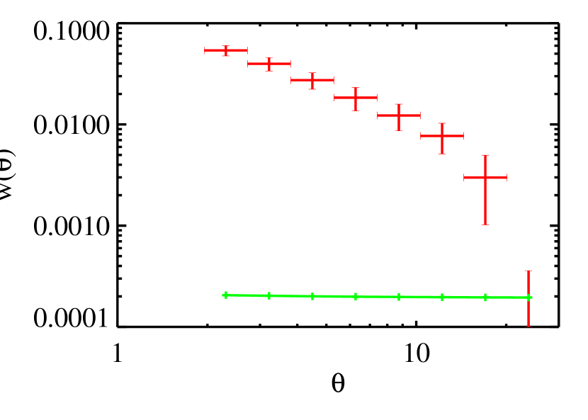
Figure 7.— The integral constraint correction, $\Delta\hat{w}(\theta)$, compared to the angular correlation function $w(\theta)$ for the pixelized estimator. The integral constraint is small because it is suppressed by a factor $N_{c}^{2}$ where in this case $N_{c}=32,512$. Thus the integral constraint is not relevant for large surveys like 2MASS and SDSS except at the largest angular scales.

4. The Angular Correlation Function

4.1. Estimators, Biases, and Errors

Following Sc02 we use two estimators for the angular correlation function. The first, which we will refer to as the pair-estimator, compares positions of the observed galaxies (data) to the positions of random points by counting the number of pairs in an angular bin $\theta_{\alpha}$ normalized by the total number of pairs. We use one million randomly placed points for the comparison, avoiding the regions that were masked as described in §3. The angular correlation can then be computed using the the now standard estimator introduced by Landy & Szalay (1993),

$$w(\theta)={{\langle DD\rangle-2\langle DR\rangle+\langle RR\rangle}\over{\langle RR\rangle}}\,,$$ (5)

where DD, DR, and RR are the normalized number of data-data, data-random and random-random pairs in an angular bin $\theta$. At large angular scales counting pairs becomes computationally expensive, so instead we calculate the galaxy density in a cell as described in §3 (eq. 3), which we refer to as the cell-estimator. Then the value of the angular correlation function is given by

$$w(\theta)={{\sum\delta^{g}_{i}\delta^{g}_{j}\Theta^{ij}_{\alpha}}\over{\sum_{ik}\Theta^{ij}_{\alpha}}},$$ (6)

where again $\Theta^{ij}_{\alpha}$ is unity if the angular separation of cell $i$ and cell $j$ is within $\theta_{\alpha}$ and zero otherwise. We use the pair-estimator for $\theta<5\arcdeg$ and the cell-estimator for $\theta>2\arcdeg$ which gives three angular bins where we use both methods to check that they generate the same results. In the overlapping regions we will use the pair-estimator which should be more accurate because the data has not been smoothed.

All estimates of $w(\theta)$ are subject to a statistical bias referred to as the “integral constraint” (Peebles, 1980; Bernstein, 1994; Hui & Gaztañaga, 1999). This bias arises because the estimate of the mean number density in a given cell enters into the estimator of the angular correlation function nonlinearly. The integral constraint correction, $\Delta\hat{w}(\theta)$, for the cell-estimator can be calculated to be (see Sc02),

$$\Delta\hat{w}(\theta_{\beta})=\left[1+(2c_{12}-3)w(\theta_{\beta})\right]\frac{1}{N_{c}^{2}}\sum_{i,j}w(\theta_{ij}),$$ (7)

where $c_{12}\approx 2$ and the sum is over all cells. Since this value is suppressed by a factor of $N_{c}^{2}$ this bias is extremely small for large surveys like 2MASS and SDSS. Figure 7 shows $\Delta\hat{w}(\theta)$ in comparison with $w(\theta)$. One clearly sees that the integral constraint can safely be ignored at all angular scales where we can measure $w(\theta)$.

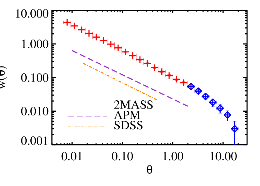
Figure 8.— The angular correlation function of 2MASS galaxies. Bins evaluated using the pixelized estimator are shown with an X, otherwise the pairs estimator is used (crosses). The errors are based on Jackknife resampling. The best-fit power laws of the APM (long dash; Maddox et al., 1990) and SDSS (dot-dash; Connolly et al., 2002) surveys are shown for comparison. The solid line is a power law with a slope of $-0.79\pm 0.02$ and an amplitude at $1\arcdeg$ of $0.10\pm 0.01$.

To calculate errors we use the Jackknife resampling method, the method that Sc02 found to be the best data-only method for estimating errors. We remove one tile of $1024$ cells and then use the two estimators described above to determine $w(\theta)$ on the remaining data set. We therefore make $N_{t}=40$ measurements of the angular correlation function in $25$ angular bins. To calculate errors we determine a covariance matrix out of the $40$ measurements. The $\alpha\beta$ element of the covariance matrix is computed by

$$C_{\alpha\beta}={{N_{t}}\over{N_{t}-1}}\sum_{k=0}^{N_{t}}\left[w_{k}(\theta_{\alpha})-\bar{w}(\theta_{\alpha})\right]\left[w_{k}(\theta_{\beta})-\bar{w}(\theta_{\beta})\right]$$ (8)

where $w_{k}(\theta_{\alpha})$ refers to the $k$th measurement of the angular correlation function on the angular scale $\theta_{\alpha}$.

Because of the strong covariance between different angular bins, it is necessary to include it when fitting a model to the data. Thus we minimize the complete form of the statistic

$$\chi^{2}=\sum_{\alpha,\beta}\left[w(\theta_{\alpha})-w_{m}(\theta_{\alpha})\right]C^{-1}_{\alpha\beta}\left[w(\theta_{\beta})-w_{m}(\theta_{\beta})\right]$$ (9)

where $w_{m}(\theta)$ is a model of the angular correlation function (see Bernstein, 1994, for a discussion).

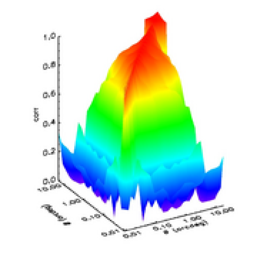
Figure 9.— The correlation matrix of the angular correlation function of 2MASS galaxies. The correlation matrix is the covariance matrix normalized by its diagonal elements. One sees that for bins less than $0.06\arcdeg$ the data is fairly independent. But at scales larger than this there is a strong correlation between different data bins.

4.2. Results

The angular correlation function of 2MASS galaxies is shown in Figure 8. We fit a power law of form $w(\theta)=A\theta^{1-\gamma}$ out to angular scales of $2.5\arcdeg$ to the estimated $w(\theta)$. Note that the uncertainties of the power-law fit are substantially underestimated if one ignores the covariance between angular bins. Hence to fit a power-law form to our estimated angular correlation function we use Singular Value Decomposition (see §5.2) to remove the oscillatory modes from the covariance matrix. We then find a best fit power law with an amplitude at $1\arcdeg$ of $A=0.10\pm 0.01$ and $1-\gamma=-0.79\pm 0.02$. However, we find that a power law is not a good fit to the angular correlation function ($\chi^{2}/{\rm d.o.f.}=2.4$ using eq. 9) using the full covariance matrix (see discussion below). As shown in Table 2, the slope of $w(\theta)$ from 2MASS is slightly higher but in overall agreement with the slopes found in APM (Maddox et al., 1990) and SDSS EDR (Connolly et al., 2002). The power-law fit to the 2MASS data extends past $\theta=1-2\arcdeg$, where the APM and EDR angular correlation functions start to deviate from a power law. This is expected since the same physical scale will correspond to a larger angular scale in the shallower 2MASS catalog.

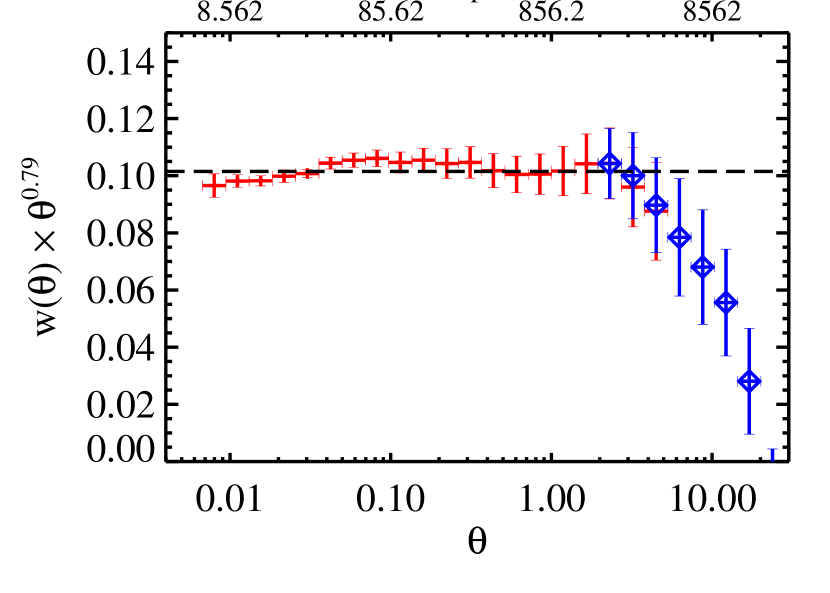
Figure 10.— The angular correlation function of 2MASS galaxies multiplied by $\theta^{0.79}$. Small oscillations around the power-law form are apparent and are statistically significant. The horizontal dashed line with amplitude $A=0.10$ is the best fit power law. Bins evaluated using the pixelized estimator are shown with an X, otherwise the pairs estimator is used (crosses).

Survey	A	1-$\gamma$	$z_{m}$	sample selection
APM	$0.028\pm 0.003$	$-0.70\pm 0.03$	$0.11$	$b_{J}<20$
SDSS	$0.013\pm 0.060$	$-0.74\pm 0.04$	$0.17$	$18<r_{*}<19$
2MASS	$0.10\pm 0.01$	$-0.79\pm 0.02$	$0.074$	$K_{s}<13.5$
2MASS	$0.08\pm 0.01$	$-0.79\pm 0.02$	$0.080$	$13.5<K_{s}<12.5$
2MASS	$0.22\pm 0.02$	$-0.79\pm 0.02$	$0.047$	$12.5<K_{s}<11.5$
2MASS	$0.48\pm 0.03$	$-0.48\pm 0.02$	$0.029$	$11.5<K_{s}<10.5$
2MASS	$0.15\pm 0.01$	$-0.79\pm 0.02$	$0.071$	$\mu_{K}<17.75$
2MASS	$0.08\pm 0.006$	$-0.76\pm 0.02$	$0.079$	$\mu_{K}>17.75$

Table 2The results of fitting the the angular correlation function with a functional form $A\theta^{1-\gamma}$ for APM (Maddox et al., 1996), SDSS (Connolly et al., 2002) and this work. We also show the fitted parameters when the 2MASS sample is divided by effective surface brightness and into magnitude bins.

The amplitude of the 2MASS angular correlation function is 3.6 (7.7) times larger than the amplitude found in the APM (SDSS EDR) surveys. We expected there would be an amplitude difference both because 2MASS galaxies are brighter than either the APM or SDSS EDR survey and because 2MASS galaxies have a shallower redshift distribution. Assuming that the galaxies in all three surveys have the same 3-dimensional power spectrum, we can use Limber’s equation (eq. 11) to calculate that the change in amplitude in $w(\theta)$ when going from the median redshift of SDSS ($0.17$) to the median redshift of 2MASS ($0.074$) is approximately a factor of 5. From Table 2 we see that the ratio of amplitudes is a factor of $7.7$, hence even after including the median redshift difference the 2MASS $w(\theta)$ amplitude is still $50\%$ higher than SDSS. We attribute the remaining amplitude offset to the difference in luminosity of the galaxies being sampled. The average ($r-K_{s})$ color of a galaxy is approximately $3.0$ so our magnitude cut of $K_{s}<13.57$ corresponds to $r<16.5$. Therefore, the faintest 2MASS galaxies are two magnitudes brighter than the mean of the brightest magnitude bin used in the SDSS study. More luminous galaxies are more clustered than less luminous ones (Norberg et al., 2001; Zehavi et al., 2002).

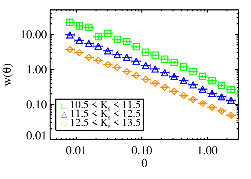
Figure 11.— The angular correlation functions of 2MASS galaxies divided into bins of $\Delta K_{s}=1$ centered on $K_{s}$=11,12,13. The error bars, which are smaller then the symbols, decrease with $K_{s}$ magnitude since there are fewer bright galaxies. The slopes remain the same while the amplitudes increase for brighter galaxies as expected.

In Figure 10, we plot the angular correlation function of 2MASS galaxies multiplied by $\theta^{0.79}$ to examine the deviations from a pure power law. The poor value of $\chi^{2}/{\rm d.o.f.}$ for the power-law fit, the straight-horizontal line, may seem surprising since the magnitude of the deviations are similar to the error bars. However, the depicted error bars follow from the diagonal elements of the correlation matrix and do not describe independent variance. Owing to significant off-diagonal terms in the covariance matrix, the displacement of adjacent $w(\theta)$ bins towards the power law fit gives a very large contribution to $\chi^{2}$. The correlation matrix of $w(\theta)$ is shown in Figure 9. The importance of off diagonal elements is clearly seen in the figure. Thus, the oscillatory behavior scene in Figure 10 is significant. These may be the result of wiggles in the power spectrum caused by baryon oscillations as recently detected in the 2dFGRS power spectrum (Percival et al., 2001). The oscillations seen here, however, are at much smaller scales then those seen in the 2dFGRS and are in the nonlinear regime. Such oscillations are expected in halo occupation distribution descriptions of galaxy clustering (Seljak, 2000; Berlind & Weinberg, 2002; Zehavi et al., 2004) and the dip centered around 0.8 degrees, corresponding to $700h^{-1}$ kpc at the median redshift of our survey, occurs at about the expected physical scale.

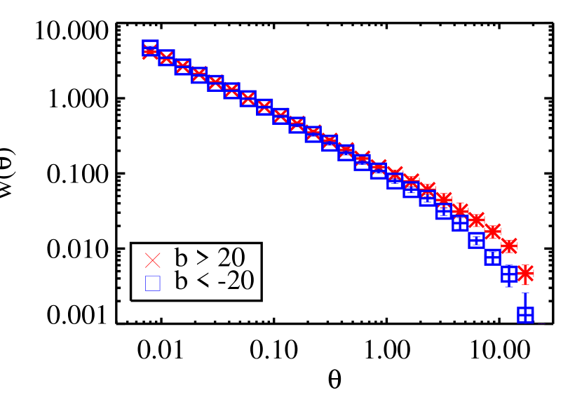
Figure 12.— The angular correlation function of 2MASS galaxies for northern Galactic latitudes ($b>20\arcdeg$ diamonds) and southern Galactic latitudes ($b<-20\arcdeg$ squares). For angular scales less then $0.5\arcdeg$ the two hemisphere yield consistent results. However, at larger angular scales there is stronger clustering in the northern Galactic hemisphere.

We also calculate the angular correlation of 2MASS galaxies split into bins of $\Delta K_{s}=1$ centered on $K_{s}$=11, 12, 13 and plot each $w(\theta)$ in Figure 11. The error bars at a given angular separation increase for brighter magnitudes owing to their lower numbers. Limber’s equation (Limber, 1953) implies that apparently brighter galaxies should have parallel $w(\theta)$ with higher amplitudes owing to their closer redshift distribution. Using the median redshift of the galaxies in each magnitude bin (see Table 2) we estimate that the amplitude ratio should be $6:2.5:1$, going from the brightest to the faintest bin. In Table 2 we present the parameters of the power-law fits to $w(\theta)$ for each magnitude bin and confirm that the differences in amplitude can be fully explained by differences in median redshift, consistent with true clustering.

Because 2MASS is an all sky survey with 1% photometric uniformity on large angular scales (Nikolaev et al., 2000), we have two independent volumes, one for northern $b>20\arcdeg$ and one for southern $b<-20\arcdeg$ Galactic latitudes. We can compute $w(\theta)$ independently for the two hemispheres as a check on our procedure and to examine the effects of cosmic variance, plotted in Figure 12. At angles less than $0.5\arcdeg$ there is good agreement. However, at larger angles the northern Galactic hemisphere shows more clustering, caused by real differences in the observed large scale structure between the northern and southern Galactic hemispheres (Maller et al., 2003, Fig. 2). For small angular scales, however, this cosmic variance is unimportant.

One would like to investigate the dependence of $w(\theta)$ on galaxy morphology. In the optical, galaxy morphology can be estimated using either galaxy color or concentration. In the infrared, however, the ($J-K_{s}$) colors contain little information about the galaxy type, since all galaxies have ($J-K_{s}$) colors that are tightly peaked around 1.0. Furthermore, Bell et al. (2003) demonstrate that the 2MASS concentration measurement is not very accurate for faint ($K_{s}>12$) galaxies. Instead, as a measure of galaxy morphology we use effective surface brightness

$$\mu_{K}=K_{s}+2.5\log_{10}{(2\pi r^{2}_{e})},$$ (10)

where $r_{e}$ is the half-light radius of the galaxy, and $K_{s}$ is the extinction-corrected Kron magnitude. For $6,238$ 2MASS galaxies also in the SDSS EDR we show in Figure 13 that $\mu_{K}$ is correlated with the SDSS optical concentration $c_{r}=r_{90}/r_{50}$, where $r_{90}$ and $r_{50}$ are the radii within which $90\%$ and $50\%$ of the galaxy flux are contained, respectively. The SDSS collaboration has adopted $c_{r}=2.6$ to separate between early and late types in a rudimentary fashion (e.g. Strateva et al., 2001; Kauffmann et al., 2003). Using $c_{r}\geq 2.6$, we find that 2630/3203 (82%) of the high surface brightness ($\mu_{K}<17.75$ mag arcsec^-2) galaxies are early-type.

Figure 13.— SDSS $r$-band concentration $c_{r}=r_{90}/r_{50}$ versus effective surface brightness $\mu_{K}=K_{s}+2.5\log_{10}{(2\pi r^{2}_{e})}$. The horizontal dotted line indicates $c_{r}=2.6$, chosen by SDSS to divide early from late-type galaxies. The vertical dashed line at $\mu_{K}<17.75$ mag arcsec^-2 shows our adopted morphology divider.

Dividing the sample at the median $\mu_{K}=17.75$, we plot the angular correlation functions of the two populations in Figure 14. The higher surface brightness galaxies are more clustered with an amplitude at $1\arcdeg$ almost twice that of the lower surface brightness galaxies (see Table 2). Unlike the difference in amplitude for the different magnitude bins, which are caused by differences in the median redshifts, our high and low surface brightness galaxies have nearly identical median redshifts of 0.079 and 0.071, respectively. Hence, the higher $\mu_{K}$ (early-type) galaxies truly are more clustered in three dimensions than the low $\mu_{K}$ (late-type) galaxies in our sample. This increased clustering amplitude for early type galaxies has also been seen in the EDR three-dimensional correlation function (Zehavi et al., 2002) and is related to the morphology-density relation (Dressler, 1980).

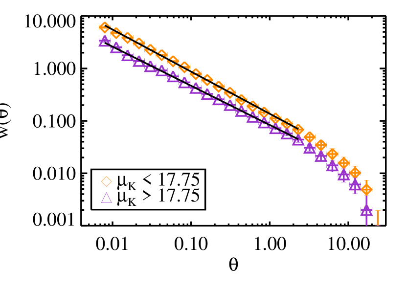
Figure 14.— The angular correlation function of high and low surface brightness 2MASS galaxies. Galaxies with $\mu_{K}<17.75$ (diamonds) are more clustered and have a slightly steeper slope than galaxies with $\mu_{K}>17.75$ (triangles).

The slopes of the two angular correlation functions are marginally different; they disagree at the $90\%$ confidence level. Such a disagreement could result from nonlocal biasing or nonlocal causes for the morphology-density relation (Narayanan et al., 2000; Scherrer & Weinberg, 1998). It would be interesting to see if any galaxy formation scenario matches this slight disagreement.

5. The 3D Power Spectrum

In this section we invert the estimated angular correlation function to measure the three-dimensional power spectrum. The relationship between $w(\theta)$ and $P(k)$ can be expressed as

$$w(\theta)=\int^{\infty}_{0}dkkP(k)g(k\theta)$$ (11)

where the kernel $g(k\theta)$ is given by

$$g(k\theta)={{1}\over{2\pi}}\int^{\infty}_{0}dzJ_{0}(k\theta X(z))(\frac{dN}{dz})^{2}{{dz}\over{dX}}F(z)$$ (12)

(Limber, 1953; Baugh & Efstathiou, 1993). In the above equation $X(z)$ is the comoving distance to a redshift $z$, $J_{0}$ is the zero order Bessel function and $F(z)$ is a function that describes the redshift evolution of density fluctuations and any evolution of the galaxy population. Following Dodelson et al. (2002) we set $F(z)=1$, which is a much better approximation for the very local 2MASS data than for other surveys. $\frac{dN}{dz}$ is the probability distribution of galaxy redshifts in the survey, i.e. the number of galaxies per redshift bin normalized to unity. The comoving distance is

$$X(z)={{c}\over{H_{0}}}\int^{z}_{0}{{dz^{\prime}}\over{E(z^{\prime})}}$$ (13)

where

$$E(z) = {{dz}\over{dX}}$$

$$= \sqrt{\Omega_{m}(1+z)^{3}+\Omega_{K}(1+z)^{2}+\Omega_{\Lambda}}$$

(Peebles, 1980). Thus, with the measured angular correlation function and knowledge of the redshift distribution of the galaxies in the survey, it is possible to estimate $P(k)$. We adopt the currently fashionable $\Lambda$CDM model (Spergel et al., 2003), $\Omega_{m}=0.3$ and $\Omega_{\Lambda}=0.7$, and note that the depth of 2MASS makes cosmological dependence small.

There are a number of methods for performing the inversion. We will use the method of Singular Value Decomposition advocated by Eisenstein & Zaldarriaga (2001), and used for the SDSS analysis of the EDR (Dodelson et al., 2002)

5.1. Redshift Distribution

To determine the redshift distribution of 2MASS galaxies we use redshifts measured by the SDSS EDR (Stoughton et al., 2002) and by the 2dFGRS 100k release (Colless et al., 2001). We identify $6,238$ 2MASS galaxies with redshifts in the SDSS EDR and $9,649$ 2MASS galaxies with redshifts in the 2dFGRS 100k release. The distribution of redshifts from the two samples (shown in Figure 15) are similar, although statistically significant differences, which are caused by the local large-scale structure, are apparent at most redshifts.

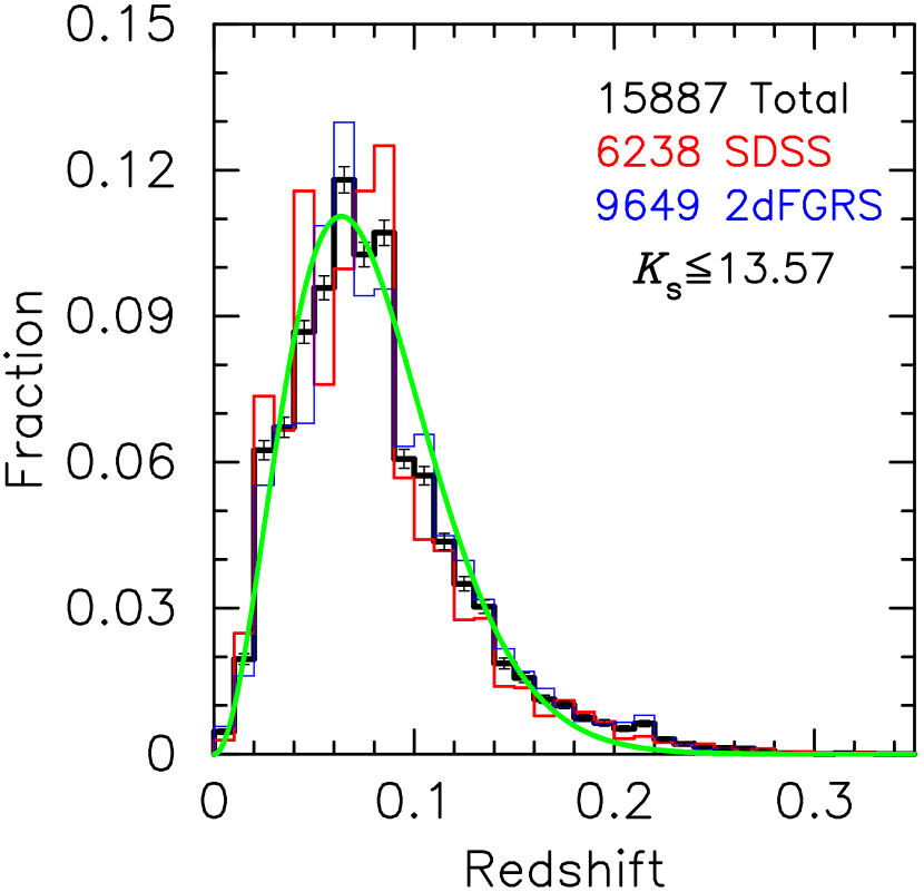
Figure 15.— Relative redshift distributions of 2MASS galaxies identified in the SDSS EDR (red, $N=6238$) and the 2dFGRS 100k release (blue, $N=9649$). The total distribution for the $15,887$ sources is given in bold with Poisson errors shown for each bin. The smooth curve is our best fit to equation (15), which has median redshift $z_{m}=0.0741$.

For the combined sample of $15,887$ redshifts we fit the functional form

$$\frac{dN}{dz}={{3z^{2}}\over{2(z_{m}/1.412)^{3}}}\exp{[-(1.412z/z_{m})^{3/2}]}$$ (15)

(Baugh & Efstathiou, 1993), where $z_{m}$ is the median redshift. We use bootstrap resampling to estimate the uncertainty in our determination of $z_{m}$ and find that $z_{m}=0.0741\pm 0.004$. This statistical uncertainty is probably a slight underestimate of the cosmic variance uncertainty as evidenced from the median redshifts of the two subsamples, which is $0.0746$ and $0.0735$ for 2dFGRS and SDSS, respectively. These are both more than one sigma from the median of the combined sample. We compare the functional form $dN/dz$ to the data in Figure 15. The kernel resulting from using this $dN/dz$ in equation 12 is shown in Figure 16.

Figure 16.— The absolute value of the kernel as a function of $k\theta$. The dashed line shows where the kernel is negative. The inversion will be most sensitive to the first zero of the kernel, which occurs at $k\theta=0.013$.

5.2. Inverting the Angular Correlation Function

In practice we measure the angular correlation function in $N_{\theta}$ bins and would like to estimate the power spectrum in $N_{k}$ bins. We can transform the integral in equation (11) into a discrete sum and write the equation in matrix form as

$$w=GP$$ (16)

where $w$ is an $N_{\theta}$ element vector containing the value of $w(\theta)$ in each bin, $P$ is an $N_{k}$ element vector containing the values of $P(k)$ in each bin, and the $N_{\theta}\times N_{k}$ matrix $G$ is a discretization of equation (11).

The inversion is thus reduced to a standard problem in linear algebra; the best fit power spectrum being given by $P=G^{-1}w$ and the power spectrum covariance matrix by $C_{P}=G^{t}C_{w}G$. Singular Value (SV) Decomposition (for a review see Press et al., 1992, §2.6 and §15.6) provides an effective method of solving and analyzing this problem. The matrix $G$ can be decomposed into $G=UWV^{t}$ where $W$ is a square diagonal matrix of the singular values and $U$ and $V$ are unitary. Then $G^{-1}$ is simply given by $G^{-1}=VW^{-1}U^{t}$. However, those elements of $W$ that are singular or very small will make a large contribution to $G^{-1}$. To remove this contribution, these eigenvalues are set to zero in the (pseudo-) inverse matrix $W^{-1}$. In practice, we remove eigenvalues that cause large oscillations in the resulting power spectrum.

Our $\theta$ bins span the range $0.00014-0.3$ radians. Since the first zero of the kernel occurs at $k\theta=0.013$, we expect sensitivity to $k$ values between $0.04-100h$ Mpc^-1. However, since small $k$ are the most interesting for cosmology as they probe the linear regime, we attempt to extend our analysis down to $k=0.004$. We use $18$ bins in wavenumber, $4$ per decade, spanning the range $0.003-100h$ Mpc^-1. Figure 17 shows the recovered power spectrum as a function of the number of modes we retain from the SV decomposition. We find that including $16$ SV modes gives us sensitivity to small $k$ but doesn’t result in wild oscillations of the power spectrum. This produces an acceptable fit to $w(\theta)$ with $\chi^{2}=4.1$ with $N_{\theta}-N_{SV}=9$ degrees of freedom.

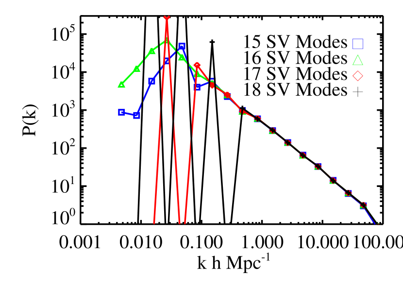
Figure 17.— The recovered power spectrum for different choices in the number of SV modes retained for the inversion. Retaining too many modes leads to wild oscillations in $P(k)$. With $16$ SV modes we are sensitive to small $k$ but do not exhibit oscillations.

In Figure 18 we plot the inferred power spectrum (with 16 SV modes) compared to the power spectra measured for SDSS (Dodelson et al., 2002, $r$-band selected) and APM (Eisenstein & Zaldarriaga, 2001, $b_{J}$-band selected). There is general agreement for the power spectra measured in all three surveys. The drop in power at $k<0.03h$ Mpc^-1 is not statistically significant as demonstrated below. The plotted error bars are the square root of the diagonal elements of the inverse covariance matrix, $\sqrt{C_{P,ii}^{-1}}$. Since the $k$ bins are not independent, they represent the uncertainty in a bin if the values of all other bins are kept fixed. They are shown only for comparison to the other surveys and to get a feel for the relative error in a given bin. To treat properly the uncertainty in the measured $P(k)$ one must use the full covariance matrix. In Table 3 we give the inverse correlation matrix, which can be used to recover the inverse covariance matrix $r^{-1}$ (contact the authors for a more precise table). The elements of the inverse correlation matrix are given by

$$r_{ij}^{-1}={{C^{-1}_{P,ij}}\over{\sqrt{C^{-1}_{P,ii}C^{-1}_{P,jj}}}}.$$ (17)

The correlation matrix is shown in Figure 19. The importance of off diagonal elements and the oscillatory nature of different $k$ bins is clearly seen.

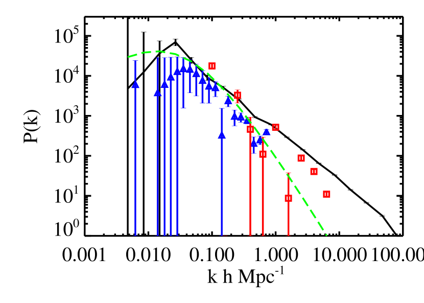
Figure 18.— The power spectrum measured from 2MASS (solid line). For comparison the results from the APM survey (triangles) as analyzed by Eisenstein & Zaldarriaga (2001), and for the $r=18-19$ magnitude bin of the SDSS survey (squares) are shown. In all cases error bars are the square root of the diagonal elements of the inverse covariance matrix, $\sqrt{C_{P,ii}^{-1}}$. The dashed line is the best fit CDM type power spectrum to the linear regime $k<0.15$. The dotted line is the power spectrum from the CMB as determined by (Spergel et al., 2003).

5.3. CDM Models

In the CDM paradigm for the evolution of the Universe, the power spectrum can be predicted based on the value of the cosmological parameters of which the most important are the matter density of the universe $\Omega_{M}$ and the Hubble constant 100$h$ Mpc^-1 kms^-1. The shape of the power spectrum is most sensitive to the combination $\Omega_{M}h$. Along with a normalization, in terms of $\sigma_{8}$ for example, this specifies a power spectrum given an initial spectral index $n_{s}$. Thus $\Omega_{M}h$ and $\sigma_{8}$ serve as a convenient parameterizations of the power spectrum on linear scales. We fit $P(k)$ inverted from $w(\theta)$ only for bins with $k<0.15h$ Mpc^-1, bins that are still in the linear regime (see Percival et al., 2001, Figure 4). We use the transfer function fitting formula of Eisenstein & Hu (1999), $n_{s}=1.0$ and take the the baryon density $\Omega_{b}=0.02h^{-2}$ in agreement with results from BBN (Kirkman et al., 2003) and the CMB (Spergel et al., 2003) We plot the best-fit power spectrum in Figure 18 including the error in the median redshift of the sample. The CDM power spectrum is a good fit to the data giving $\chi^{2}/{\rm d.o.f.}=0.6$. Hence, the apparent drop in power on large scales, as seen by some authors (Gaztanaga & Baugh, 1998; Allgood et al., 2001), is not statistically significant.

The constraints on $\sigma_{8}$ and $\Omega_{M}h$ are shown in Figure 20. We find $\sigma_{8}=1.0\pm 0.1$ and $\Omega_{M}h=0.13\pm 0.07$ ($95\%$ confidence limits). One must remember that this is only a parameterized fit to the power spectrum of $K_{s}<13.57$ galaxies; any relation to cosmology requires an understanding of how galaxies trace the underlying dark matter density field. The 2dfGRS find a power spectrum best fit by $\Omega_{m}h=0.2\pm 0.03$ (Percival et al., 2001) consistent with our measurement.

In comparison, cosmological parameters measured from the WMAP satellite alone give $\Omega_{M}h=0.19\pm 0.03$, $\sigma_{8}=0.9\pm 0.1$ and $n_{s}=.99$ (Spergel et al., 2003). This would imply a $K_{s}$-band linear bias of $b_{K}=1.1\pm 0.2$ in good agreement with the $K_{s}$-band bias determined from the 2MASS clustering dipole of $b_{K}=1.37\pm 0.34$ (Maller et al., 2003).

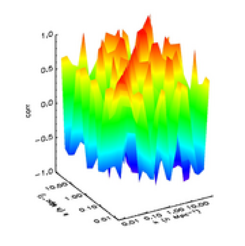
Figure 19.— The correlation matrix of the power spectrum measured from 2MASS. The correlation matrix is the covariance matrix normalized by its diagonal elements. One sees how different $k$ bins are not at all independent but are all interwoven in an oscillatory fashion. The elements of the correlation matrix are also given in Table 3.

6. Conclusions

We have presented a measurement of the angular correlation function and three-dimensional power spectrum for galaxies from the 2MASS catalog. We have minimized the contribution of the possible contaminants of stars, dust, seeing and sky brightness by studying their cross-correlation with the galaxy density and making cuts in the data until these cross-correlations are less then the auto-correlation signal. These restrictions on the data limit us to $|b|>20\arcdeg$ and dust extinctions $\Delta K_{S}<0.05$. More than a half million galaxies remain for estimating the angular correlation function.

The best fit power law to the measured angular correlation function has a slope of $-0.79\pm 0.02$ and an amplitude at one degree of $0.10\pm 0.01$ out to $2.5\arcdeg$. There are oscillations around this power law that are statistically significant. The largest oscillation occurs at about 0.8 degrees, corresponding to $700h^{-1}$ kpc at the median redshift of our survey, as expected in halo occupation distribution descriptions of galaxy clustering (Seljak, 2000; Berlind & Weinberg, 2002; Zehavi et al., 2004). The slope of this power law is in good agreement with other determinations of $w(\theta)$ (Maddox et al., 1996; Connolly et al., 2002). We divide the sample into three magnitude bins and estimate the angular correlation function for each magnitude bin. We confirm that differences in the $w(\theta)$ amplitude at these three brightnesses is fully explained by differences in the median redshift, consistent with true clustering. We partition the data by northern and southern Galactic latitude and see that at large angles the northern Galactic latitudes show a greater correlation amplitude, caused by the observed large structures of the Virgo super cluster and the Shapley concentration in the northern Galactic hemisphere (see Maller et al., 2003, Fig. 2). We also partition the data by effective surface brightness and find that galaxies with higher surface brightness are more clustered, which is a manifestation of the morphology-density relation (Dressler, 1980). Their $w(\theta)$ may also have a slightly steeper slope and might be evidence for nonlocal biasing.

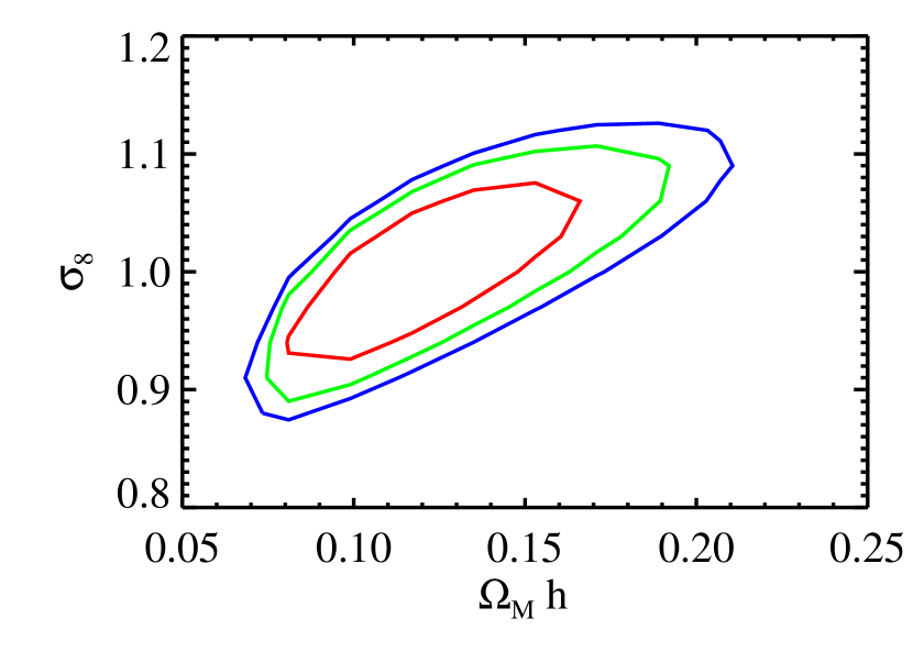
Figure 20.— The $66.7\%,95\%$ and $99\%$ confidence intervals in the $\sigma_{8}$ — $\Omega_{M}h$ plane from fitting to our derived $P(k)$. Projecting onto one-dimension gives constraints of $\sigma_{8}=1.0\pm 0.1$ and $\Omega_{M}h=0.13\pm 0.07$.

We solve for the three-dimensional power spectrum from the angular correlation function using Singular Value Decomposition. Our resulting power spectrum is in good agreement with other measurements using the same method (Eisenstein & Zaldarriaga, 2001; Dodelson et al., 2002). The best fit CDM power spectra gives values of $\Omega_{M}h=0.13\pm 0.07$ and $\sigma_{8}=1.0\pm 0.1$, assuming a spectral index of $1.0$. This fit is to the galaxy power spectrum and its relation to cosmological parameters will depend on how galaxies trace the underlying mass distribution. The ratio of our measured $\sigma_{8}$ to that determined from WMAP (Spergel et al., 2003) would imply a $K_{s}$ band linear bias of $b_{K}=1.1\pm 0.2$.

Our $K_{s}$-band selected power spectrum, is in good agreement with other determinations of the power spectrum in surveys selected in other wavebands in the linear regime. On smaller length scales there is a significant difference between other galaxy power spectra and that measured for $K_{s}$-band selected galaxies. Thus the power spectrum measured here, in combination with the power spectrum measured from the CMB and other large galaxy surveys, will enable one to place strong constraints on theories of galaxy formation.

$k$	0.0047	0.0084	0.015	0.027	0.047	0.084	0.15	0.27	0.47	0.84	1.5	2.7	4.7	8.4	15.	27.	47.	84.
$P(k)$	4792.2	12419.1	36534.2	69942.7	24786.4	9083.5	5107.2	2508.1	928.1	606.5	290.9	141.6	65.2	33.1	14.2	6.7	3.2	0.9
$\sqrt{C_{P,ii}^{-1}}$	2.9E-06	8.9E-06	2.6E-05	7.4E-05	2.3E-04	7.2E-04	2.6E-03	8.4E-03	2.7E-02	6.6E-02	1.5E-01	3.5E-01	1.1E+00	1.9E+00	2.8E+00	6.1E+00	9.3E+00	8.1E+00
	1.00	1.00	0.98	0.83	0.51	0.43	0.01	-0.32	-0.05	-0.18	-0.25	0.16	0.43	0.08	-0.16	-0.41	-0.29	0.26
	1.00	1.00	0.99	0.86	0.55	0.44	0.02	-0.31	-0.07	-0.21	-0.25	0.18	0.43	0.06	-0.17	-0.39	-0.27	0.25
	0.98	0.99	1.00	0.92	0.65	0.48	0.06	-0.30	-0.13	-0.29	-0.26	0.23	0.42	-0.02	-0.19	-0.34	-0.20	0.21
	0.83	0.86	0.92	1.00	0.87	0.58	0.16	-0.25	-0.28	-0.50	-0.27	0.33	0.36	-0.20	-0.20	-0.18	-0.02	0.11
	0.51	0.55	0.65	0.87	1.00	0.77	0.30	-0.18	-0.38	-0.59	-0.35	0.28	0.36	-0.27	-0.14	-0.08	0.04	0.10
	0.43	0.44	0.48	0.58	0.77	1.00	0.57	-0.14	-0.22	-0.29	-0.49	0.08	0.59	0.07	-0.02	-0.33	-0.32	0.33
	0.01	0.02	0.06	0.16	0.30	0.57	1.00	0.36	-0.06	-0.12	-0.23	0.04	0.16	0.09	0.05	-0.00	-0.01	0.02
	-0.32	-0.31	-0.30	-0.25	-0.18	-0.14	0.36	1.00	0.41	-0.14	-0.11	-0.18	-0.29	-0.01	0.57	0.45	0.02	-0.50
	-0.05	-0.07	-0.13	-0.28	-0.38	-0.22	-0.06	0.41	1.00	0.59	-0.11	-0.47	-0.03	0.44	0.29	0.01	-0.29	-0.01
	-0.18	-0.21	-0.29	-0.50	-0.59	-0.29	-0.12	-0.14	0.59	1.00	0.04	-0.42	0.06	0.62	0.02	-0.26	-0.29	0.20
	-0.25	-0.25	-0.26	-0.27	-0.35	-0.49	-0.23	-0.11	-0.11	0.04	1.00	0.31	-0.37	-0.16	0.06	0.24	0.11	-0.14
	0.16	0.18	0.23	0.33	0.28	0.08	0.04	-0.18	-0.47	-0.42	0.31	1.00	0.33	-0.23	-0.06	-0.02	0.03	-0.16
	0.43	0.43	0.42	0.36	0.36	0.59	0.16	-0.29	-0.03	0.06	-0.37	0.33	1.00	0.48	-0.02	-0.57	-0.53	0.28
	0.08	0.06	-0.02	-0.20	-0.27	0.07	0.09	-0.01	0.44	0.62	-0.16	-0.23	0.48	1.00	0.22	-0.52	-0.52	0.14
	-0.16	-0.17	-0.19	-0.20	-0.14	-0.02	0.05	0.57	0.29	0.02	0.06	-0.06	-0.02	0.22	1.00	0.27	-0.34	-0.44
	-0.41	-0.39	-0.34	-0.18	-0.08	-0.33	-0.00	0.45	0.01	-0.26	0.24	-0.02	-0.57	-0.52	0.27	1.00	0.49	-0.76
	-0.29	-0.27	-0.20	-0.02	0.04	-0.32	-0.01	0.02	-0.29	-0.29	0.11	0.03	-0.53	-0.52	-0.34	0.49	1.00	-0.35
	0.26	0.25	0.21	0.11	0.10	0.33	0.02	-0.50	-0.01	0.20	-0.14	-0.16	0.28	0.14	-0.44	-0.76	-0.35	1.00

Table 3The results of the best fit power spectrum using 16 SV modes. The first row are the centers of the $k$ bins in $h$ Mpc^-1. The second row are the best fit values of $P(k)$. The third row is the square root of the covariance matrix, $\sqrt{C_{P,ii}}$. The fourth row is the square root of the inverse covariance matrix $\sqrt{C_{P,ii}^{-1}}$ and the rest of the table gives the $18\times 18$ symmetric inverse correlation matrix $r^{-1}$ (see text). Note redshift errors are not included in the above. For a table with greater precision please contact the authors.

References

- Allgood et al. (2001) Allgood, B., Blumenthall, G. R., & Primack, J. R. 2001, in Where’s the Matter?, ed. L. Tresse & M. Treyer, 197, astro-ph/0109403
- Baugh & Efstathiou (1993) Baugh, C. M. & Efstathiou, G. 1993, MNRAS, 265, 145
- Bell et al. (2003) Bell, E. F., McIntosh, D. H., Katz, N., & Weinberg, M. D. 2003, ApJS, 149, 289
- Berlind & Weinberg (2002) Berlind, A. A. & Weinberg, D. H. 2002, ApJ, 575, 587
- Bernstein (1994) Bernstein, G. M. 1994, ApJ, 424, 569
- Boschán (2002) Boschán, P. 2002, MNRAS, 334, 297
- Cole et al. (2001) Cole, S. et al. 2001, MNRAS, 326, 255
- Colless et al. (2001) Colless, M. et al. 2001, MNRAS, 328, 1039
- Collins et al. (1992) Collins, C. A., Nichol, R. C., & Lumsden, S. L. 1992, MNRAS, 254, 295
- Connolly et al. (2002) Connolly, A. J. et al. 2002, ApJ, 579, 42
- Dodelson & Gaztañaga (2000) Dodelson, S. & Gaztañaga, E. 2000, MNRAS, 312, 774
- Dodelson et al. (2002) Dodelson, S. et al. 2002, ApJ, 572, 140
- Dressler (1980) Dressler, A. 1980, ApJ, 236, 351
- Efstathiou & Moody (2001) Efstathiou, G. & Moody, S. J. 2001, MNRAS, 325, 1603
- Eisenstein & Hu (1999) Eisenstein, D. J. & Hu, W. 1999, ApJ, 511, 5
- Eisenstein & Zaldarriaga (2001) Eisenstein, D. J. & Zaldarriaga, M. 2001, ApJ, 546, 2
- Gaztanaga & Baugh (1998) Gaztanaga, E. & Baugh, C. M. 1998, MNRAS, 294, 229
- Groth & Peebles (1977) Groth, E. J. & Peebles, P. J. E. 1977, ApJ, 217, 385
- G rski et al. (1999) G rski, K. M., Hivon, E., & Wandelt, B. D. 1999, in Evolution of Large-Scale Structure, ed. A. J. Banday, R. K. Sheth, & L. D. Costa (Garching:ESO), 37, astro-ph/9812350
- Hui & Gaztañaga (1999) Hui, L. & Gaztañaga, E. 1999, ApJ, 519, 622
- Jarrett et al. (2003) Jarrett, T. H., Chester, T., Cutri, R., Schneider, S., & Huchra, J. P. 2003, AJ, 125, 525
- Jarrett et al. (2000a) Jarrett, T.-H., Chester, T., Cutri, R., Schneider, S., Rosenberg, J., Huchra, J. P., & Mader, J. 2000a, AJ, 120, 298
- Jarrett et al. (2000b) Jarrett, T. H., Chester, T., Cutri, R., Schneider, S., Skrutskie, M., & Huchra, J. P. 2000b, AJ, 119, 2498
- Kauffmann et al. (2003) Kauffmann, G. et al. 2003, MNRAS, 341, 33
- Kirkman et al. (2003) Kirkman, D., Tytler, D., Suzuki, N., O’Meara, J. M., & Lubin, D. 2003, ApJS, 149, 1
- Kochanek et al. (2001) Kochanek, C. S. et al. 2001, ApJ, 560, 566
- Kron (1980) Kron, R. G. 1980, ApJS, 43, 305
- Landy & Szalay (1993) Landy, S. D. & Szalay, A. S. 1993, ApJ, 412, 64
- Limber (1953) Limber, D. N. 1953, ApJ, 117, 134
- Lucy (1974) Lucy, L. B. 1974, AJ, 79, 745
- Maddox et al. (1996) Maddox, S. J., Efstathiou, G., & Sutherland, W. J. 1996, MNRAS, 283, 1227
- Maddox et al. (1990) Maddox, S. J., Efstathiou, G., Sutherland, W. J., & Loveday, J. 1990, MNRAS, 242, 43
- Maller et al. (2003) Maller, A. H., McIntosh, D. H., Katz, N., & Weinberg, M. D. 2003, ApJ, 598, L1
- Narayanan et al. (2000) Narayanan, V. K., Berlind, A. A., & Weinberg, D. H. 2000, ApJ, 528, 1
- Nikolaev et al. (2000) Nikolaev, S., Weinberg, M. D., Skrutskie, M. F., Cutri, R. M., Wheelock, S. L., Gizis, J. E., & Howard, E. M. 2000, AJ, 120, 3340, calibration
- Norberg et al. (2001) Norberg, P. et al. 2001, MNRAS, 328, 64
- Padilla & Baugh (2003) Padilla, N. D. & Baugh, C. M. 2003, MNRAS, 343, 796
- Peebles (1980) Peebles, P. J. E. 1980, The large-scale structure of the universe, Princeton Series in Physics (New Jersey: Princeton University Press)
- Percival et al. (2001) Percival, W. J. et al. 2001, MNRAS, 327, 1297
- Press et al. (1992) Press, W. H., Teukolsky, S. A., Vetterling, W. T., & Flannery, B. P. 1992, Numerical recipes in FORTRAN. The art of scientific computing (Cambridge: University Press, —c1992, 2nd ed.)
- Scherrer & Weinberg (1998) Scherrer, R. J. & Weinberg, D. H. 1998, ApJ, 504, 607
- Schlegel et al. (1998) Schlegel, D. J., Finkbeiner, D. P., & Davis, M. 1998, ApJ, 500, 525
- Scranton et al. (2002) Scranton, R. et al. 2002, ApJ, 579, 48, [Sc02]
- Seljak (2000) Seljak, U. 2000, MNRAS, 318, 203
- Skrutskie et al. (1997) Skrutskie, M. F. et al. 1997, in ASSL Vol. 210: The Impact of Large Scale Near-IR Sky Surveys, ed. F. G. et al. (Kluwer Academic Publishing Company, Dordrecht), 25–32
- Spergel et al. (2003) Spergel, D. N. et al. 2003, ApJS, 148, 175
- Stoughton et al. (2002) Stoughton, C. et al. 2002, AJ, 123, 485
- Strateva et al. (2001) Strateva, I. et al. 2001, AJ, 122, 1861
- Strauss et al. (2002) Strauss, M. A. et al. 2002, AJ, 124, 1810
- York et al. (2000) York, D. G. et al. 2000, AJ, 120, 1579
- Zehavi et al. (2002) Zehavi, I. et al. 2002, ApJ, 571, 172
- Zehavi et al. (2004) —. 2004, ApJ, 608, 16
- Zwicky & Kowal (1968) Zwicky, F. & Kowal, C. T. 1968, in CGCG6, 0