The Halo Distribution of 2dF Galaxies

Abstract

We use the clustering results obtained by Madgwick et al. (2003) for a sample of 96,791 2dF galaxies with redshift $0.01<z<0.15$ to study the distribution of late-type and early-type galaxies within dark matter haloes of different mass. Within the framework of our models, galaxies of both classes are found to be as spatially concentrated as the dark matter within haloes even though, while the distribution of star-forming galaxies can also allow for some steeper profiles, this is drastically ruled out in the case of early-type galaxies. We also find evidence for morphological segregation, as late-type galaxies appear to be distributed within haloes of mass scales corresponding to groups and clusters up to about two virial radii, while passive objects show a preference to reside closer to the halo centre. If we assume a broken power-law of the form $\langle N_{\rm gal}\rangle(m)=(m/m_{0})^{\alpha_{1}}$ for $m_{\rm cut}\leq m<m_{0}$ and $\langle N_{\rm gal}\rangle(m)=(m/m_{0})^{\alpha_{2}}$ at higher masses to describe the dependence of the average number of galaxies within haloes on the halo mass, fits to the data show that star-forming galaxies start appearing in haloes of masses $m_{\rm cut}\simeq 10^{11}m_{\odot}$, much smaller than what is obtained for early-type galaxies ($m_{\rm cut}\simeq 10^{12.6}m_{\odot}$). In the high-mass regime $m\geq m_{0}$, $\langle N_{\rm gal}\rangle$ increases with halo mass more slowly ($\alpha_{2}\simeq 0.7$) in the case of late-type galaxies than for passive objects which present $\alpha_{2}\simeq 1.1$. The above results imply that late-type galaxies dominate the 2dF counts at all mass scales. We stress that – at variance with previous statements – there is no degeneracy in the determination of the best functional forms for $\rho(r)$ and $\langle N_{\rm gal}\rangle$, as they affect the behaviour of the galaxy-galaxy correlation function on different scales.

1 Introduction

Measurements of the galaxy-galaxy correlation function contain a wealth of information both on the underlying cosmological model and on the physical processes connected with the formation and evolution of galaxies. Untangling these two effects from the observed clustering signal of a particular class of sources is, however, not an easy task. For instance, the physics of galaxy formation affects the relationship between the distribution of luminous and dark matter (the so-called “bias”) so that different types of galaxies are expected to exhibit different clustering properties. This has indeed been observed (see e.g. Loveday et al., 1995; Guzzo et al., 1997; Loveday, Tresse & Maddox, 1999; Magliocchetti et al., 2000 just to mention few) in the past decade, when large-area surveys started including enough sources to allow for precision clustering statistics.

From a theoretical point of view, the relationship between dark matter and galaxy distribution has not yet fully been understood since, while the dynamics of dark matter is only driven by gravity and fully determined by the choice of an appropriate cosmological model (see e.g. Jenkins et al., 1998), the situation gets increasingly more difficult as one tries to model the physical processes playing a role in the process of galaxy formation.
As a first approximation, galaxies can be associated with the dark matter haloes in which they reside (in a one-to-one relationship), so that their clustering properties can be derived within the framework of the halo-model developed by Mo & White (1996). Such models have been proved extremely useful to describe the clustering of high-redshift sources such as quasars, Lyman Break and SCUBA galaxies (see e.g. Matarrese et al., 1997; Moscardini et al., 1998; Martini & Weinberg, 2001; Magliocchetti et al., 2001; Porciani & Giavalisco, 2002) where the assumption of one such object per halo can be considered a reasonable guess.
The validity of this approach however breaks down as one moves to objects with higher number densities such as low-redshift galaxies. The distribution of these kind of sources within dark matter haloes is in general an unknown quantity which will depend on the efficiency of galaxy formation via some complicated physics connected to processes such as gas cooling and/or supernova feedback (see e.g. Somerville et al., 2001; Benson et al., 2001).

The analytical connection between the distribution of sources within dark matter haloes and their clustering properties has been studied in detail by a number of recent papers (Peacock & Smith, 2000; Seljak, 2000; Scoccimarro et al., 2001; Bullock, Wechsler & Somerville 2002; Marinoni & Hudson, 2002; Berlind & Weinberg, 2001; Moustakas & Somerville, 2002; Yang, Mo & van den Bosch 2003; van den Bosch, Yang & Mo, 2003; see also Cooray & Sheth, 2002 for an extensive review on the topic) which mainly focus on the issue of the halo occupation function i.e. the probability distribution of the number of galaxies brighter than some luminosity threshold hosted by a virialized halo of given mass. Within this framework, the distribution of galaxies within haloes is shown to determine galaxy-galaxy clustering on small scales, being responsible for the observed power-law behaviour at separations $r\mathrel{\hbox to0.0pt{\lower 3.0pt\hbox{$\sim$}\hss}\raise 2.0pt\hbox{$<$}}3$ Mpc.

A number of parameters are necessary to describe the halo occupation distribution (i.e. the probability of finding $N_{\rm gal}$ galaxies in a halo of mass $m$) of a class of galaxies. These parameters – expected to vary with galaxy type – cannot be worked out from first principles and have to rely for their determination either on comparisons with results from semi-analytical models or on statistical measurements coming from large data-sets, with an obvious preference for this second approach.
The two last-generation 2dF and SDSS Galaxy Redshift Surveys (Colless et al., 2001; York et al., 2000) come in our help since – with their unprecedented precision in measuring galaxy clustering – they can in principle constrain the functional form of the halo occupation distribution (see also Zehavi et al., 2003).

Lower-order clustering measurements such as the spatial two-point correlation function are already available for samples of 2dF sources (Norberg et al., 2001; Hawkins et al., 2003; Madgwick et al., 2003). In this work we will use the results of Madgwick et al. (2003) on the clustering properties of late-type and early-type galaxies to investigate possible differences in the processes responsible for the birth and evolution of these two classes of sources.

The layout of the paper is as follows: Section 2 introduces the formalism necessary to describe galaxy clustering within the halo occupation distribution context. Key ingredients for this kind of analysis are the average number $\langle N_{\rm gal}\rangle(m)$ of galaxies hosted in dark matter haloes of mass $m$, a measure of the spread $\langle N_{\rm gal}(N_{\rm gal}-1)\rangle(m)$ about this mean value and the spatial distribution $\rho(r)$ of galaxies within their haloes. In Section 3 we briefly describe the 2dF Galaxy Redshift Survey with particular attention devoted to measurements of the luminosity function and correlation function for early-type (i.e. passively evolving) and late-type (which are still in the process of active star formation) galaxies, and derive estimates for the number density of these sources. Section 4 presents and discusses our results on the distribution of different types of galaxies within dark matter haloes as obtained by comparing predictions on their number density and correlation function with 2dF observations, while Section 5 summarizes our conclusions.

Unless differently stated, throughout this work we will assume that the density parameter $\Omega_{0}=0.3$, the vacuum energy density $\Lambda=0.7$, the present-day value of the Hubble parameter in units of $100$ km/s/Mpc $h_{0}=0.65$ and $\sigma_{8}=0.8$ (with $\sigma_{8}$ the rms linear density fluctuation within a sphere with a radius of $8h^{-1}$ Mpc), as the latest results from the joint analysis of CMB and 2dF data seem to indicate (see e.g. Lahav et al., 2002; Spergel et al., 2003). Note, however, that the normalization of the linear power spectrum of density fluctuations is still very controversial: estimates of $\sigma_{8}$ from either weak-lensing or cluster abundances range between 0.6 and 1.0, while some analyses of galaxy clustering seem to favour values $\sim 0.7$ (van den Bosch, Mo & Yang 2003). Our results will slightly depend on the assumed value for $\sigma_{8}$.

2 Galaxy Clustering: The Theory

The purpose of this Section is to introduce the formalism and specify the ingredients necessary to describe galaxy clustering at the 2-point level. Our approach follows the one adopted by Scoccimarro et al. (2001) which is in turn based on the analysis performed by Scherrer & Bertschinger (1991). In this framework, the galaxy-galaxy correlation function can be written as

$$\xi_{g}({\bf x}-{\bf x}^{\prime})=\xi_{g}^{1h}({\bf x}-{\bf x}^{\prime})+\xi_{g}^{2h}({\bf x}-{\bf x}^{\prime}),$$ (1)

with

$$\xi_{g}^{1h}=\frac{1}{\bar{n}_{g}^{2}}\int n(m)\langle N_{\rm gal}(N_{\rm gal}-1)\rangle(m)dm\times$$

$$\int\rho_{m}({\bf y})\rho_{m}({\bf y}+{\bf x}-{\bf x}^{\prime})d^{3}y,$$ (2)

and

$$\xi_{g}^{2h}=\frac{1}{\bar{n}_{g}^{2}}\int n(m_{1})\langle N_{\rm gal}\rangle(m_{1})dm_{1}\times\;\;\;\;\;\;\;\;\;\;\;\;\;\;\;\;\;\;\;\;\;\;\;\;\;\;\;\;$$ (3)

$$\int n(m_{2})\langle N_{\rm gal}\rangle(m_{2})dm_{2}\int\rho_{m_{1}}({\bf x}-{\bf x}_{1})d^{3}x_{1}$$

$$\times\int\rho_{m_{2}}({\bf x}^{\prime}-{\bf x}_{2})\xi({\bf x}_{1}-{\bf x}_{2};m_{1},m_{2})d^{3}x_{2},\;\;\;\;\;\;\;\;\;\,$$

where the first term $\xi_{g}^{1h}$ accounts for pairs of galaxies residing within the same halo, while the $\xi_{g}^{2h}$ represents the contribution coming from galaxies in different haloes. Note that all the above quantities are dependent on the redshift $z$, even though we have not made it explicit.
In the above equations, $\langle N_{\rm gal}\rangle(m)$ is the mean number of galaxies per halo of mass $m$, and $\langle N_{\rm gal}(N_{\rm gal}-1)\rangle(m)$ – also dependent on the mass of the halo hosting the galaxies – is a measure of the spread about this mean value. The mean comoving number density of galaxies is defined as:

$$\bar{n}_{g}=\int n(m)\langle N_{\rm gal}\rangle(m)dm,$$ (4)

where $n(m)$ is the halo mass function which gives the number density of dark matter haloes per unit mass and volume. $\xi({\bf x}_{1}-{\bf x}_{2};m_{1},m_{2})$ is the two-point cross-correlation function between haloes of mass $m_{1}$ and $m_{2}$ and, finally, $\rho_{m}({\bf y})$ is the (spatial) density distribution of galaxies within the haloes, normalized so to obtain

$$\int_{0}^{r_{\rm cut}}\rho_{m}({\bf y})d^{3}y=1,$$ (5)

where $r_{\rm cut}$ is the radius which identifies the outer boundaries of the halo.

From the above discussion it then follows that, in order to work out $\xi_{g}$, we need to specify the halo-halo correlation function, the halo mass function, the spatial distribution of galaxies within the haloes and a functional form for the number distribution of galaxies within the haloes. This is done as follows.

2.1 Halo-Halo Correlation Function

An approximate model for the 2-point correlation function of dark–matter haloes can be easily obtained from the mass autocorrelation function as (see e.g. Porciani & Giavalisco, 2002)

$$\xi({\bf r},z,m_{1},m_{2})=\;\;\;\;\;\;\;\;\;\;\;\;\;\;\;\;\;\;\;\;\;\;\;\;\;\;\;\;\;\;\;\;\;\;\;\;\;\;\;\;\;\;\;\;\;\;\;\;\;\;\;\;\;\;$$

$$=\left\{\begin{array}[]{ll}\xi_{dm}(r,z)b_{1}(m_{1},z)b_{2}(m_{2},z)\;\;\;{\rm if}\;r\geq r_{1}+r_{2}\\ -1\;\;\;\;\;\;\;\;\;\;\;\;\;\;\;\;\;{\rm otherwise},\end{array}\right.$$ (8)

where the above expression takes into account the halo-halo spatial exclusion ($r_{1}=r_{\rm cut_{1}}$ and $r_{2}=r_{\rm cut_{2}}$ are the Eulerian radii of the collapsed haloes, in general identified with their virial radii), and the mass-mass correlation function $\xi_{dm}(r,z)$ – fully specified for a given cosmological model and a chosen normalization of $\sigma_{8}$ – has been calculated following the approach of Peacock & Dodds (1996) which is sufficiently accurate both in the linear and non-linear regimes. In fact, results obtained with the more precise algorithm developed by Smith et al. (2003) significantly differ from those obtained with the method by Peacock & Dodds (1996) only in the regime where the 1-halo term dominates the 2-point clustering signal.

The linear bias factor $b(m,z)$ of individual haloes of mass $m$ at redshift $z$ can instead be written as (Sheth & Tormen, 1999; see also Cole & Kaiser 1989; Mo & White 1996; Catelan et al. 1997; Porciani et al. 1998)

$$b(m,z)=1+\frac{a\nu-1}{\delta_{c}}+\frac{2p/\delta_{c}}{1+(a\nu)^{p}},$$ (9)

with $p=0.3$, $a=0.707$, $\nu=(\delta_{c}/\sigma)^{2}$, where $\delta_{c}\simeq 1.686$ and $\sigma$ respectively are the critical overdensity for collapse and the linear rms variance of the power spectrum on the mass scale $m$ at redshift $z$.

Note that, at variance with previous works (e.g. Peacock & Smith, 2000; Seljak, 2000; Scoccimarro et al.,2001; Berlind & Weinberg, 2001) where the halo-halo correlation function was only derived in the linear regime, our equation (8) fully accounts for the non-linear evolution of density fluctuations. Using linear theory to compute the 2-halo term can be considered as a good approximation on large scales ($r\mathrel{\hbox to0.0pt{\lower 3.0pt\hbox{$\sim$}\hss}\raise 2.0pt\hbox{$>$}}5$ Mpc) – where the clustering growth is indeed still linear – and does not create any problems on small scales ($r\mathrel{\hbox to0.0pt{\lower 3.0pt\hbox{$\sim$}\hss}\raise 2.0pt\hbox{$<$}}1$ Mpc) – where the 1-halo term $\xi_{g}^{1h}$ dominates the clustering signal. It, however, breaks down at intermediate distances where the $\xi_{g}^{1h}$ and $\xi_{g}^{2h}$ contributions are of comparable importance. It follows that the use of a linear halo-halo correlation function in equation (3) systematically leads to a serious underestimate of the clustering signal (1) produced by low-$z$ galaxies on scales $1\mathrel{\hbox to0.0pt{\lower 3.0pt\hbox{$\sim$}\hss}\raise 2.0pt\hbox{$<$}}r/[\rm Mpc]\mathrel{\hbox to0.0pt{\lower 3.0pt\hbox{$\sim$}\hss}\raise 2.0pt\hbox{$<$}}5$, when compared with results obtained by taking into account the fully non-linear behaviour of $\xi_{dm}(r,z)$. For this reason, we believe our approach to be more consistent than the ones adopted so far. We note that similar models – unknown to us till the very last stages of the present paper – have also been used by Zehavi et al. (2003), Yang et al. (2003) and van den Bosch et al. (2003).

2.2 Mass Function

For the analytical expression of the halo mass function we rely once again on the Sheth & Tormen (1999) form:

$$n(m,z)=\frac{A\bar{\rho}}{m^{2}}\sqrt{\frac{a\nu}{2\pi}}\left(1+\frac{1}{(a\nu)^{p}}\right)\exp{\left(-\frac{a\nu}{2}\right)}\left|\frac{d({\rm ln}\nu)}{d({\rm ln}{\it m})}\right|$$ (10)

(with $A=0.322$, $\bar{\rho}$ the mean background density and the other quantities defined as above), since it gives an accurate fit to the results of N-body simulations with the same initial conditions (Jenkins et al. 2001; Sheth, Mo & Tormen 2001).

2.3 Spatial Distribution of Galaxies

The first, easiest approach one can take for the spatial distribution of galaxies within a halo of specified mass $m$ is to assume that galaxies follow the dark matter profile. Under this hypothesis we can then write

$$\rho^{\prime}_{m}(r)=\rho_{m}(r)\cdot m=\bar{\rho}\;\frac{fc^{3}/3}{cr/r_{\rm vir}(1+cr/r_{\rm vir})^{2}},$$ (11)

where we use the Navarro, Frenk & White (1997, hereafter NFW) expression, which provides a good description of the density distribution within virialized haloes in numerical simulations. In equation (11), $r_{\rm vir}$ is the virial radius of the halo, related to its mass via $m=(4\pi r_{\rm vir}^{3}/3)\Delta\bar{\rho}$, where $\Delta$ (=340 for an $\Omega=0.3$ universe at $z=0$) is the characteristic density contrast of virialized systems; $f=\Delta/[\rm{ln(1+c)-c/(1+c)}]$, and for the concentration parameter $c$ we use equations (9) and (13) in Bullock et al. (2001).

Clearly, the assumption for the distribution of galaxies within virialized haloes to trace the dark matter profile is not necessarily true. For instance, the semi-analytic models by Diaferio et al. (1999) suggest that this cannot hold for both late-type and early-type galaxies since blue galaxies tend to reside in the outer regions of their parent haloes, while red galaxies are preferentially found near the halo centre.
For this reason, in the following analysis we will also consider spatial distributions of the form $\rho_{m}^{\prime}(r)\propto(r/r_{\rm vir})^{-\beta}$, with $\beta=2,2.5,3$, where the first value corresponds to the singular isothermal sphere case.

The last remark concerns the choice for values of $r_{\rm cut}$ in equations (5) and (8). All the profiles (both the NFW and the power-laws) considered so far formally extend to infinity, leading to divergent values for the associated masses. This implies the need to “artificially” truncate the distribution profiles at some radius $r_{\rm cut}$. One sensible choice is to set $r_{\rm cut}\equiv r_{\rm vir}$, since one expects galaxies to form within virialized regions, where the overdensity is greater than a certain threshold. However, this might not be the only possible choice since for instance – as a consequence of halo-halo merging – galaxies might also be found in the outer regions of the newly-formed halo, at a distance from the center greater than $r_{\rm vir}$.

The way different assumptions for the steepness of the profiles and different choices for $r_{\rm cut}$ affect the galaxy-galaxy correlation function on small scales ($r\mathrel{\hbox to0.0pt{\lower 3.0pt\hbox{$\sim$}\hss}\raise 2.0pt\hbox{$<$}}1$ Mpc) is presented in Figure (1). To this particular aim, both $\xi_{g}^{1h}$ and $\xi_{g}^{2h}$ have been derived from equation (1) by setting $\langle N_{\rm gal}\rangle=\langle N_{\rm gal}(N_{\rm gal}-1)\rangle=1$ for all halo masses greater than $10^{10.7}m_{\sun}$ and 0 otherwise.
The two panels show the case for $r_{\rm cut}=r_{\rm vir}$ (top) and $r_{\rm cut}=2\cdot r_{\rm vir}$ (bottom), while solid, short-dashed, long-short-dashed and dotted lines respectively represent the results for a NFW, a power-law with $\beta=2.5$, a power-law with $\beta=2$ and a power-law with $\beta=3$ distribution profiles. Lower curves (for $r\to 0$) correspond to the $\xi_{g}^{2h}$ term (contribution from objects in different haloes), while the upper ones indicate the $\xi_{g}^{1h}$ term.
As Figure (1) clearly shows, both the scale at which the transition from a regime where objects in different haloes dominate the clustering signal to a regime where galaxies within the same halo start giving a contribution and the amplitudes of the $\xi_{g}^{1h}$ and $\xi_{g}^{2h}$ terms greatly depend on the radius chosen to truncate the distribution profiles. More in detail, the amplitude of both terms decreases and differences between predictions obtained for different profiles become more pronounced as the value for $r_{\rm cut}$ increases. Finally note that – independently of the value of $r_{\rm cut}$ – a stronger clustering signal at small scales is in general expected for steeper density profiles.

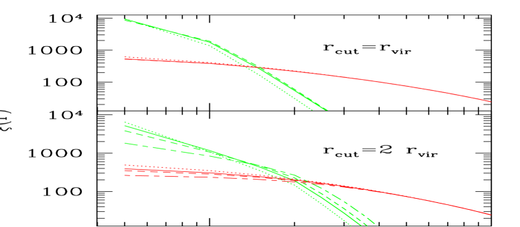
Figure 1: Results for the galaxy-galaxy correlation function as obtained from different assumptions for the galaxy distribution profiles $\rho(r)$ and different choices for $r_{\rm cut}$. The case for $r_{\rm cut}=r_{\rm vir}$ is shown in the top panel, while the one for $r_{\rm cut}=2\cdot r_{\rm vir}$ is presented in the bottom panel. Solid, short-dashed, long-short-dashed and dotted lines represent the predictions for a NFW, a power-law with $\beta=2.5$, a power-law with $\beta=2$ and power-law with $\beta=3$ distribution runs. Lower curves correspond to the term $\xi_{g}^{2h}$ in equation (1) (contribution from objects in different haloes), while the upper ones indicate the $\xi_{g}^{1h}$ term. All the above curves have been calculated by setting in equation (1) $\langle N_{\rm gal}\rangle=\langle N_{\rm gal}(N_{\rm gal}-1)\rangle=1$ for all halo masses greater than $10^{10.7}m_{\sun}$ and 0 otherwise.

Results originating from different assumptions for a spatial distribution of galaxies within dark matter haloes and different truncation radii will be further investigated in the following sections.

2.4 Halo Occupation Function

A key ingredient in the study of the clustering properties of galaxies is their halo occupation function $p(N_{\rm gal}|m)$ which gives the probability for a halo of specified mass $m$ to contain $N_{\rm gal}$ galaxies. In the most general case, $p(N_{\rm gal}|m)$ is entirely specified by the knowledge of its $n$ moments $\langle N^{n}_{\rm gal}\rangle(m)$ which in principle can be observationally determined by means of the so-called “counts in cells” analysis (see e.g. Benson, 2001). Unfortunately this is not feasible in reality, as measures of the higher moments of the galaxy distribution get extremely noisy for $n>4$ even for 2-dimensional catalogues (see e.g. Gaztanaga, 1995 for an analysis of the APM survey).
A possible way to overcome this problem is to rely on the lower-order moments of the galaxy distribution to determine the low-order moments of the halo occupation function, and then assume a functional form for $p(N_{\rm gal}|m)$ in order to work out all the higher moments (see e.g. Scoccimarro et al., 2001; Berlind & Weinberg, 2002). Clearly, better and better determinations of $p(N_{\rm gal}|m)$ are obtained as we manage to estimate higher and higher moments of the galaxy distribution function.

Since this work relies on measurements of the two-point correlation function of 2dF galaxies, equation (1) shows that in our case only the first and second moment of the halo occupation function can be determined from the data, as these are the only two quantities which play a role in the theoretical description of $\xi_{g}$.
Following Scoccimarro et al. (2001), we chose to write the mean number of galaxies per halo of specified mass $m$ as

$$\langle N_{\rm gal}\rangle(m)=0\;\;\;\;\;\;\;\;\;\;\;\;\;\;\;\;\;\;\;\;\;\;\;\;\;\;\;\;\;\;\rm{if}\;\;{\it m<m}_{\rm cut}$$

$$\langle N_{\rm gal}\rangle(m)=(m/m_{0})^{\alpha_{1}}\;\;\;\;\;\;\rm{if}\;\;{\it m}_{\rm cut}\leq{\it m<m}_{0}$$ (12)

$$\langle N_{\rm gal}\rangle(m)=(m/m_{0})^{\alpha_{2}}\;\;\;\;\;\;\;\;\;\;\;\;\;\;\;\rm{if}\;\;{\it m\geq m}_{0},,$$

where $m_{\rm cut}$, $m_{0}$, $\alpha_{1}$ and $\alpha_{2}$ are parameters to be determined by comparison with observations. The choice of the above functional form for $\langle N_{\rm gal}\rangle(m)$ relies on the physics connected with galaxy formation processes (see e.g. Benson et al., 2001; Somerville et al., 2001; Sheth & Diaferio, 2001). For instance, $m_{\rm cut}$ gives the minimum mass of a halo able to host a galaxy since – for potential wells which are not deep enough – galaxy formation is inhibited by supernova processes occurring amongst the first stars which can blow the remaining gas away from the halo itself therefore suppressing further star-formation. On the other hand, given that the internal velocity dispersion of haloes increases with halo mass, gas is expected to cool less efficiently and therefore inhibit at some level galaxy formation in more massive haloes. In a hierarchical scenario for structure formation, however, the most massive objects are formed by merging and accretion of smaller units. Thus, one expects the number of galaxies to increase with the halo size in the high-mass regime. All this can then be parameterized by a broken power-law of the form (10), with $m_{0}$ the “threshold mass” at which the transition between the two different scaling laws occurs.

The last ingredient needed for the description of 2-point galaxy clustering is the second moment of the halo occupation function appearing in equation (1). This term quantifies the spread (or variance) about the mean value of the number counts of galaxies in a halo. A convenient parameterization for this quantity is:

$$\langle N_{\rm gal}(N_{\rm gal}-1)\rangle(m)=\alpha(m)^{2}\langle N_{\rm gal}\rangle^{2},$$ (13)

where $\alpha(m)=0,{\rm log}(m/m_{\rm cut})/{\rm log}(m_{0}/m_{\rm cut}),1$, respectively for $m<m_{\rm cut}$, $m_{\rm cut}\leq m<m_{0}$ and $m\geq m_{0}$. Note that, while the high-mass value for $\alpha(m)$ simply reflects a Poissonian statistics, the functional form at intermediate masses (chosen to fit the results from semi-analytical models – see e.g. Sheth & Diaferio, 2001; Berlind & Weinberg 2002 – and smoothed particle hydrodynamics simulations – Berlind et al. 2003) describes the sub-Poissonian regime.


As a last consideration, note that equation (1) presents in both the $\xi_{g}^{1h}$ and $\xi_{g}^{2h}$ terms convolutions of density profiles. Since this is somehow difficult to deal with, we prefer to work in Fourier space where all the expressions simply become multiplications over the Fourier transforms of the profiles. Equation (1) is therefore equivalent to:

$$\bar{n}^{2}_{g}\Delta_{g}(k)=\int n(m)\langle N_{\rm gal}(N_{\rm gal}-1)\rangle(m)|u_{m}(k)|^{2}dm+$$

$$\int u_{m_{1}}(k)\langle N_{\rm gal}\rangle(m_{1})n(m_{1})dm_{1}\times\;\;\;\;\;\;\;\;\;\;\;\;\;\;\;\;\;$$

$$\int u_{m_{2}}(k)n(m_{2})\langle N_{\rm gal}\rangle(m_{2})\Delta(k,m_{1},m_{2})dm_{2},$$ (14)

where – allowing for the exclusion effects as in equation (6) – $\Delta(k,m_{1},m_{2})=\Delta_{dm}(k)b(m_{1})b(m_{2})$ is the power spectrum of haloes of mass $m_{1}$ and $m_{2}$ ($\Delta_{dm}(k)=k^{3}/(2\pi^{2})P_{dm}(k)$ is the normalized non-linear power-spectrum for dark matter – (see e.g. Peacock & Dodds, 1996),

$$u_{m}(k)=\frac{k^{3}}{(2\pi^{2})}\int_{0}^{r_{\rm cut}}\rho_{m}(r){\rm sin}(kr)/(kr)4\pi r^{2}dr,$$ (15)

with $\rho_{m}(r)$ defined as in (5), is the Fourier transform of the galaxy distribution profile truncated at $r_{\rm cut}$, and where all the quantities are implicitly taken at a fixed $z$. In this framework, the galaxy-galaxy correlation function can then be obtained from equation (14) via

$$\xi_{g}(r)=\int\Delta_{g}(k)\frac{{\rm sin}(kr)}{kr}\frac{dk}{k}.$$ (16)

3 The 2dF Galaxy Redshift Survey

The 2dF Galaxy Redshift Survey (2dFGRS: Colless et al., 2001) is a large-scale survey aimed at obtaining spectra for 250,000 galaxies to an extinction-corrected limit for completeness of $b_{J}=19.45$ over an area of 2151 square degrees. The survey geometry consists of two broad declination strips, a larger one in the SGP covering the area $3^{h}30^{m}\mathrel{\hbox to0.0pt{\lower 3.0pt\hbox{$\sim$}\hss}\raise 2.0pt\hbox{$<$}}{\rm RA}({\rm 2000})\mathrel{\hbox to0.0pt{\lower 3.0pt\hbox{$\sim$}\hss}\raise 2.0pt\hbox{$<$}}21^{h}40^{m}$, $-37.5^{\circ}\mathrel{\hbox to0.0pt{\lower 3.0pt\hbox{$\sim$}\hss}\raise 2.0pt\hbox{$<$}}{\rm dec}({\rm 2000})\mathrel{\hbox to0.0pt{\lower 3.0pt\hbox{$\sim$}\hss}\raise 2.0pt\hbox{$<$}}-22.5^{\circ}$ and a smaller one set in the NGP with $9^{h}50^{m}\mathrel{\hbox to0.0pt{\lower 3.0pt\hbox{$\sim$}\hss}\raise 2.0pt\hbox{$<$}}{\rm RA}({\rm 2000})\mathrel{\hbox to0.0pt{\lower 3.0pt\hbox{$\sim$}\hss}\raise 2.0pt\hbox{$<$}}14^{h}50^{m}$, $2.5^{\circ}\mathrel{\hbox to0.0pt{\lower 3.0pt\hbox{$\sim$}\hss}\raise 2.0pt\hbox{$<$}}{\rm dec}({\rm 2000})\mathrel{\hbox to0.0pt{\lower 3.0pt\hbox{$\sim$}\hss}\raise 2.0pt\hbox{$<$}}-7.5^{\circ}$, plus 100 random 2-degree fields spread uniformly over the 7000 square degrees of the APM catalogue in the southern Galactic hemisphere.

The input catalogue for the survey is a revised version of the APM galaxy catalogue (Maddox et al. 1990a, 1990b, 1996) which includes over 5 million galaxies down to $b_{J}=20.5$. Redshifts for all the sources brighter than $b_{J}=19.45$ are determined in two independent ways, via both cross-correlation of the spectra with specified absorption-line templates (Colless et al., 2001) and by emission-line fitting. These automatic redshift estimates have then been confirmed by visual inspection of each spectrum, and the more reliable of the two results chosen as the final redshift. A quality flag was assigned to each redshift: $Q=3$, $Q=4$ and $Q=5$ correspond to reliable redshift determination, $Q=2$ means a probable redshift and $Q=1$ indicates no redshift measurement. The success rate in redshift acquisition for the surveyed galaxies (determined by the inclusion in the 2dF sample of only those objects with quality flags $Q=3$ to $Q=5$) is estimated about 95 per cent (Folkes et al., 1999). The median redshift of the galaxies is 0.11 and the great majority of them have $z<0.3$.

3.1 Luminosity Functions and Number Densities

Madgwick et al. (2002) calculate the optical $b_{j}$ luminosity function (LF) for different subsets of $\rm{M}-5\rm{log_{10}}(h_{0})\leq-13$ 2dFGRS galaxies defined by their spectral type. The spectral classification – based upon a Principal Component Analysis – was performed for 75,589 galaxies found at redshifts $0.01<z<0.15$ and allowed to divide the whole population into four well-defined classes according to the strength of their star-formation activity: from type 1 (early-type galaxies only showing absorption lines in their spectra) to type 4 (extremely active star-forming galaxies).

Fitting functions for the different luminosity distributions are presented in Madgwick et al. (2002) and can be used to determine the average number density of galaxies of different spectral types via (see e.g. Lin et al., 1996):

$$\bar{n}_{g_{i}}=N_{i}\times\left[\int_{z_{\rm min}}^{z_{\rm max}}S_{i}(z)(dV/dz)dz\right]^{-1},$$ (17)

with the selection function $S_{i}(z)$ defined as

$$S_{i}(z)=\frac{\int^{\rm{min[M^{\it i}_{max}(z)-M_{max}]}}_{\rm{max[M^{\it i}_{min}(z)-M_{min}]}}\Phi_{i}(\rm{M})d{\rm M}}{\int_{\rm{M_{min}}}^{\rm{M_{max}}}\Phi_{i}(\rm{M})d{\rm M}},$$ (18)

where $dV/dz$ is the volume element, $i=1,2,3,4$ refers to the spectral class, $N_{i}$ is the total number of galaxies belonging to a specific type found in the survey and $\Phi_{i}$ is their luminosity function. $\rm{M_{min}=-13+5log_{10}}(h_{0})$ , $z_{\rm min}=0.01$ and $\rm{M_{max}\simeq-21+5log_{10}}(h_{0})$, $z_{\rm max}=0.15$ respectively are the minimum and maximum absolute magnitudes and redshifts of the objects under exam, while ${\rm M^{\it i}_{min(max)}}(z)=b_{\rm max(min)}-25-5{\rm log}(d_{L}^{i})-k_{i}(z)$, where $k_{i}(z)$ is the K-correction, $d_{L}^{i}$ the luminosity distance and $b_{\rm min}=14$, $b_{\rm max}=19.45$ are the apparent magnitude limits of the 2dF survey.

We have then applied equation (17) to the four different galaxy types and found:

$$\bar{n}_{g_{1}}=9.6\cdot 10^{-3}\left\{\begin{array}[]{ll}-4.4\cdot 10^{-3}\\ +7.0\cdot 10^{-2}\end{array}\right.$$ (21)

$$\bar{n}_{g_{2}}=0.0103\pm 3\cdot 10^{-4}\;\;\;\;\;\;\;\;\;\;\;\;\;\;$$

$$\bar{n}_{g_{3}}=0.015\left\{\begin{array}[]{ll}-8\cdot 10^{-4}\\ +9\cdot 10^{-4}\end{array}\right.\;\;\;\;\;\;\;\;\;$$ (24)

$$\bar{n}_{g_{4}}=0.018\pm 1.8\cdot 10^{-3},\;\;\;\;\;\;\;\;\;\;\;\;$$

where the quoted 1$\sigma$ errors, in all but the type 1 case, are obtained by varying the ’break’ luminosities ${\rm M}^{*}_{i}$ and the faint-end slopes $\mu_{i}$ of the Schechter functions $\Phi_{i}(\rm M)=(0.4\>{\rm ln}10)\Phi^{*}_{i}(10^{-0.4({\rm M-M^{*}_{\it i}})})^{1+\mu_{i}}\rm{exp}(-10^{-0.4(M-M^{*}_{\it i})})$ (note that our calculations are independent of the normalizations $\Phi^{*}_{i}$) along their joint 1$\sigma$ error ellipse.

Two features have to be noticed in (17). First, errors on $\bar{n}_{g_{1}}$ – especially the upper 1$\sigma$ limit of the number density – are significantly larger than those derived for the other three classes of sources. This is due to the fact that the Schechter function might not provide a good fit to the faint end of the LF of type 1 galaxies (Madgwick et al., 2002); an extra term of the form $\Phi({\rm M})=10^{a+b\rm{M}}$ is needed for $\rm{M-5log_{10}}(h_{0})\mathrel{\hbox to0.0pt{\lower 3.0pt\hbox{$\sim$}\hss}\raise 2.0pt\hbox{$>$}}-16$, where the parameters $a$ and $b$ can only be determined from the data with quite large uncertainties. Since it is the faint end of the LF which mostly contributes to the determination of $\bar{n}_{g_{1}}$, and this is the region where the errors on $a$ and $b$ dominate over those derived for the various parameters in the Schechter function, this explains our finding for such large uncertainties associated to the measurement of $\bar{n}_{g_{1}}$.
The second point to be noticed concerns the errors associated to $\bar{n}_{g_{4}}$. In fact it turns out that, also in the case of type 4 galaxies, the Schechter function does not provide a good fit to the faint end of the luminosity function as it systematically overestimates the number density of $\rm{M-log_{10}}(h_{0})\mathrel{\hbox to0.0pt{\lower 3.0pt\hbox{$\sim$}\hss}\raise 2.0pt\hbox{$>$}}-16$ galaxies. This implies that the total number of type 4 sources as derived from integration of the LF is in agreement with the observed one only if we subtract to the best estimate $\bar{n}_{g_{4}}$ in eq. (17) an error corresponding to a 3$\sigma$ confidence level in $\mu_{4}$. Since, as we will see better in the next Section, the observed number density of galaxies plays a relevant role in the determination of the best halo occupation model, we have then decided in the case of type 4 sources to consider errors on $\mu_{4}$ at the 3$\sigma$ level; this propagates to a lower limit for $\bar{n}_{g_{4}}=0.0127$.

Finally, from the luminosity function we can also determine another quantity which will be useful in the following Sections: the effective redshift of a class of sources defined as $z_{i}^{\rm eff}=\int_{z_{\rm min}}^{z_{\rm max}}zS_{i}(z)(dV/dz)dz$. Numbers obtained for the different types of galaxies under exam then read: $z_{1}^{\rm eff}=0.098$, $z_{2}^{\rm eff}=0.091$, $z_{3}^{\rm eff}=0.082$, $z_{4}^{\rm eff}=0.078$, indicating a preference for late-type galaxies to be found at lower redshifts than early-type objects.

3.2 Correlation Functions

A sample with the same selection criteria as the one introduced in Section 3.1 but containing more (96,791) objects has been used by Madgwick et al. (2003) to calculate the clustering properties of galaxies belonging to different spectral types. In order to increase the statistics associated to the measurements, galaxies have been grouped into two broad categories: early-types – 36318 objects with effective redshift 0.1 to be identified with those sources belonging to spectral class 1 – and late-type – 60473 objects with effective redshift 0.09 obtained by taking into account all galaxies from spectral classes 2 3 and 4 – ones.

The different observed correlation functions are shown in Figures (2) and (6) for early-type and late-type galaxies, respectively. In order to get rid of redshift distortions, the correlation function in real space has been inferred by computing the bi-dimensional correlation parallel and transverse to the line-of-sight, $\xi_{g}(r_{P},r_{T})$, and by integrating it in the $r_{P}$ direction. The quantity presented in Figures (2) and (6) therefore corresponds to

$$\bar{\xi}_{g}(r_{T})=2\int_{r_{T}}^{\infty}\xi_{g}(r)\frac{rdr}{(r^{2}-r_{T}^{2})^{1/2}}.$$ (25)

Error-bars have been obtained by bootstrap resampling, adapting the method presented by Porciani & Giavalisco (2002).

Measurements for the integrated correlation function (25) differ for the two populations not only in their amplitude, but also in the slopes (Madgwick et al., 2003 – by fitting the data with a power-law $\xi(r)=(r/r_{0})^{\gamma}$ – find $r_{0}=3.67\pm 0.30$  h^-1 Mpc, $\gamma=1.60\pm 0.04$ for late-type galaxies and $r_{0}=6.10\pm 0.34$ h^-1 Mpc, $\gamma=1.95\pm 0.03$ for early-type sources). As we will extensively see in the next Sections, these differences can provide a great amount of information on the processes associated to galaxy formation in the two different cases of passive and active star-forming galaxies.

4 Results

In order to determine the best values for the parameters describing the halo occupation number (10) we allowed them to vary within the following region:

$$-1\leq\alpha_{1}\leq 2;\;\;\;\;\;\;\;\;\;\;\;\;\;\;$$

$$-1\leq\alpha_{2}\leq 2;\;\;\;\;\;\;\;\;\;\;\;\;\;\;$$

$$10^{9}\;m_{\odot}\leq m_{{\rm cut}}\leq 10^{13}\;m_{\odot};$$

$$m_{{\rm cut}}\leq m_{0}\leq m_{{\rm cut}}\cdot 10^{3}.\;\;\;$$

Combinations of these four quantities have then been used to evaluate the mean number density of galaxies $\bar{n}_{g}$ via equation (4). Only values for $\bar{n}_{g}$ within 2$\sigma$ from the observed ones (quoted in Section 3.1) were accepted and the corresponding values for $\alpha_{1}$, $\alpha_{2}$, $m_{\rm cut}$ and $m_{0}$ have subsequently been plugged into equation (1) to produce – for a specified choice of the distribution profile and effective redshift $z^{\rm eff}$ (slightly different in the case of early-type and late-type galaxies) – the predicted galaxy-galaxy correlation function to be integrated via eq. (25) and compared with the data by means of a least squares ($\chi^{2}$) fit.

The value for the truncation radius of the halo was set to $r_{\rm vir}$ and the above procedure repeated for different choices of $\rho_{m}(r)$. The following sub-sections describe the results obtained for the two different classes of Early- and Late-type galaxies.

4.1 Early-type galaxies

The best description of the data in this case is provided by a model with $\alpha_{1}\simeq-0.2$, $\alpha_{2}=1.1$, $m_{\rm cut}=10^{12.6}m_{\odot}$, $m_{0}=10^{13.5}m_{\odot}$ (in good agreement with the findings of Zehavi et al., 2003) and with a mild preference for galaxies to be distributed within their dark matter haloes according to a NFW profile. The projected galaxy-galaxy correlation function for this combination of values and the NFW spatial distribution is illustrated by the solid curve in Figure (2), while the dashed and dotted lines respectively indicate the contribution $\xi_{g}^{2h}$ from galaxies residing in different haloes and the $\xi_{g}^{1h}$ term originating from galaxies within the same halo. The agreement between data and predictions is good at all scales even though the model tends to underestimates the correlation function at intermediate scales (between 3 and 10 Mpc), where the maximum discrepancy is $\sim 20$ per cent.

Figure 2: Projected correlation function of early-type galaxies. Data-points represent the results from Madgwick et al. (2003), while the solid curve is the best fit to the measurements obtained for a halo number density of the form (10), with $\alpha_{1}=-0.2$, $\alpha_{2}=1.1$, $m_{\rm cut}=10^{12.6}m_{\odot}$, $m_{0}=10^{13.5}m_{\odot}$ and for galaxies distributed within their dark matter haloes according to a NFW profile. Dashed and dotted lines respectively indicate the contribution $\xi_{g}^{2h}$ from galaxies residing in different haloes and the $\xi_{g}^{1h}$ term originating from galaxies within the same halo.

A more quantitative assessment of the goodness of the match can be found in Table 1 which – for each choice of the distribution profile $\rho_{m}(r)$ and for the different classes of early-type and late-type galaxies – provides the value of the $\chi^{2}=\chi^{2}_{min}$ obtained for the best fit to the data and the corresponding estimates for the parameters which appear in the description of the halo occupation number (10). 1$\sigma$ errors on these quantities are obtained by requiring their different combinations not to produce models for the galaxy-galaxy correlation function which – when compared to the measurements – correspond to $\chi^{2}$ values which differ from the minimum by a factor greater than $\Delta\chi^{2}=3.53$, where this last figure has been derived for an analysis with three degrees of freedom (assuming Gaussian errors). Three is in fact the number of degrees obtained if one subtracts to the number of independent $\bar{\xi}_{g}$ measurements (eight – Darren Madgwick, private communication) the number of parameters to determine (four) and the (one) constraint on $\bar{n}_{g}$.

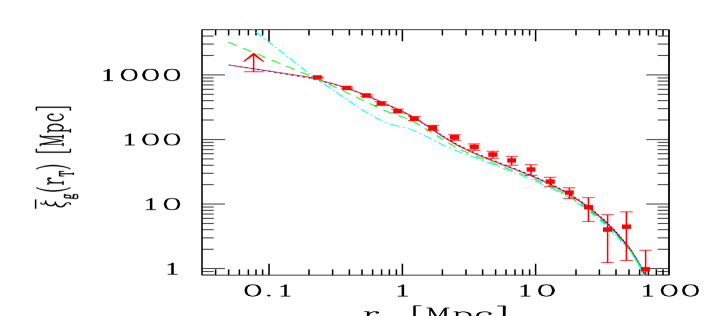
Figure 3: Projected correlation function of early-type galaxies. Data-points represent the results from Madgwick et al. (2003), while solid, dashed, dotted and dashed-dotted curves illustrate the best-fit models respectively obtained for a NFW, a power-law with $\beta=2.5$, a power-law with $\beta=2$ and a power-law with $\beta=3$ galaxy distribution profiles (see text for details). The arrow shows the lower limit to the measured correlation function set on small scales by fibre collisions in the 2dF survey (Ed Hawkins, private communication).

A closer look to Table 1 shows that, in the case of early-type galaxies, the best-fit values for the parameters appearing in equation (10) are independent – except for the most extreme cases of very poor fits – of the particular choice for the spatial distribution of galaxies within the haloes. This is verified even though different profiles are associated to different values for $\chi^{2}_{min}$ and is due to the fact that, while quantities such as $\langle N_{\rm gal}\rangle$ and $\langle N_{\rm gal}^{2}\rangle$ (and therefore the parameters associated to them) mainly determine the amplitudes of the $\xi_{g}^{1h}$ and $\xi_{g}^{2h}$ terms, the distribution of galaxies within the haloes is directly responsible for the slope of $\xi_{g}$, especially on scales $r\mathrel{\hbox to0.0pt{\lower 3.0pt\hbox{$\sim$}\hss}\raise 2.0pt\hbox{$<$}}1$ Mpc.
This effect is better seen in Figure (3) which presents the best-fit models obtained for different choices of the distribution run. More in detail, the solid line is for a NFW profile, the dotted line for a power-law profile with $\beta=2$, the dashed line for a power-law profile with $\beta=2.5$ and the dashed-dotted line represents the case of a power-law profile with $\beta=3$. Even though all the curves are almost indistinguishable from each other on all scales $r\mathrel{\hbox to0.0pt{\lower 3.0pt\hbox{$\sim$}\hss}\raise 2.0pt\hbox{$>$}}2$ Mpc due to the very similar best-fit values obtained for the parameters which describe $\langle N_{{\rm gal}}\rangle$ and $\langle N_{{\rm gal}}(N_{{\rm gal}}-1)\rangle$, this does not hold any longer at smaller distances. In fact, when we push the analysis inside the haloes, the profile assumes a crucial importance; for instance, in the case of early-type galaxies it is clear that, while profiles such as NFW and singular isothermal sphere can provide a good fit to the observations (with a slight preference for the first model), anything steeper than these two is drastically ruled out by the data since it does not exhibit enough power on scales $0.3\mathrel{\hbox to0.0pt{\lower 3.0pt\hbox{$\sim$}\hss}\raise 2.0pt\hbox{$<$}}r/[\rm{Mpc}]\mathrel{\hbox to0.0pt{\lower 3.0pt\hbox{$\sim$}\hss}\raise 2.0pt\hbox{$<$}}2$.

Table 1 states the same conclusion from a more quantitative point of view showing that, while the NFW profile provides the best description of the data and the value of $\chi^{2}_{min}$ for a $\beta=2$ model is still within the 1$\sigma$ range of the acceptable fits (for Gaussian errors), profiles of the form power-law with $\beta\mathrel{\hbox to0.0pt{\lower 3.0pt\hbox{$\sim$}\hss}\raise 2.0pt\hbox{$>$}}2.5$ are too steep to be accepted as satisfactory descriptions of the observed galaxy correlation function. We remark once again that, since the spatial distribution of galaxies within haloes of specified mass and their mean number and variance affect different regions of the observed correlation function, these two effects are untangled so that there is no degeneracy in the determination of the $\langle N_{\rm gal}\rangle$ and $\rho(r)$ preferred by the data.

Since different profiles lead to notably different predictions for the correlation function on increasingly smaller ($r\mathrel{\hbox to0.0pt{\lower 3.0pt\hbox{$\sim$}\hss}\raise 2.0pt\hbox{$<$}}0.2$ Mpc, see Figure 3) scales, one would in principle like to be able to explore this region in order to put stronger constraints on the distribution of galaxies within their haloes. Unfortunately, this cannot be done because – as Hawkins et al. (2003) have shown – fibre collisions in the 2dF survey can significantly decrease the measured $\xi_{g}(r)$ on scales $r\mathrel{\hbox to0.0pt{\lower 3.0pt\hbox{$\sim$}\hss}\raise 2.0pt\hbox{$<$}}0.1$ Mpc, leading to systematic underestimates. Nevertheless, one can still use the 2dF measurements of the correlation function as a lower limit to the real galaxy-galaxy clustering strength, to be compared with predictions steaming from different density runs. This is done in Figure 3, where the arrow represents the 2dF measurement of the early-type correlation function on a scale $r\simeq 0.07$ Mpc. In this particular case, all the models appear to have enough power on such small scales as none of them falls below the accepted range of variability of the measured $\xi_{g}(r)$. Therefore, on the basis of the present data, we cannot break the degeneracy between NFW and PL2 profiles as to which one can provide the best description of the data in the whole $r$ range.

Table 1: Best-fit values for the parameters describing the halo occupation number (10), expressed for different choices of the distribution profile and truncation radius. PL2, PL2.5 and PL3 respectively correspond to profiles described by power-laws with slopes $\beta=2$, $\beta=2.5$ and $\beta=3$. Errors are for a 68.3% confidence level and three degrees of freedom. $\bar{n}_{g}$ (in Mpc^-3) and b are the average number density of sources and the bias on large scales as derived from the combination of the best-fit parameters associated to each model. All the masses are measured in $m_{\odot}$ units. Vanishing errorbars mean that either the best-fitting value lies on the boundary of the sampled parameter space (e.g. when $\alpha_{1}=-1$) or that the uncertainty is smaller than our grid step (0.1 for all parameters).

EARLY-TYPE	NFW	PL2	PL2.5	PL3
$r_{\rm cut}=r_{\rm vir}$	$\chi_{min}^{2}=4.0$	$\chi_{min}^{2}=4.9$	$\chi_{min}^{2}=13.2$	$\chi_{min}^{2}=68.9$
	$\alpha_{1}=-0.2^{+0.6}_{-0.5}$	$\alpha_{1}=-0.5^{+1.0}_{-0.3}$	$\alpha_{1}=-0.6^{+0.7}_{-0.4}$	$\alpha_{1}=-0.5^{+0.1}_{-0.5}$
	$\alpha_{2}=1.1^{+0.1}_{-0.2}$	$\alpha_{2}=1.0^{+0.1}_{-0.1}$	$\alpha_{2}=1.5^{+0.0}_{-0.2}$	$\alpha_{2}=1.8^{+0.0}_{-0.6}$
	${\rm Log}[m_{\rm cut}]=12.6_{-0.5}^{+0.1}$	${\rm Log}[m_{\rm cut}]=12.7_{-0.7}^{+0.0}$	${\rm Log}[m_{\rm cut}]=12.7_{-0.4}^{+0.2}$	${\rm Log}[m_{\rm cut}]=12.7^{+0.2}_{-0.2}$
	${\rm Log}[m_{0}]=13.5_{-0.5}^{+0.0}$	${\rm Log}[m_{0}]=13.4_{-0.4}^{+0.1}$	${\rm Log}[m_{0}]=13.7_{-0.3}^{+0.1}$	${\rm Log}[m_{0}]=13.9_{-0.4}^{+0.1}$
	$\rm n_{g}=8.4\cdot 10^{-4}$	$\rm n_{g}=8.6\cdot 10^{-4}$	$\rm n_{g}=1.31\cdot 10^{-3}$	$\rm n_{g}=1.34\cdot 10^{-3}$
	b=1.33	b=1.34	b=1.31	b=1.30
LATE-TYPE	NFW	PL2	PL2.5	PL3
$r_{\rm cut}=r_{\rm vir}$	$\chi_{min}^{2}=90.4$	$\chi_{min}^{2}=107.6$	$\chi_{min}^{2}=81.7$	$\chi_{min}^{2}=38.8$
$r_{\rm cut}=2\;r_{\rm vir}$	$\chi_{min}^{2}=9.7$	$\chi_{min}^{2}=7.2$	$\chi_{min}^{2}=10.7$	$\chi_{min}^{2}=14.4$
	$\alpha_{1}=-0.4^{+2.4}_{-0.6}$	$\alpha_{1}=-1.0^{+3.0}_{-0.0}$	$\alpha_{1}=-0.6^{+2.4}_{-0.4}$	$\alpha_{1}=-0.7^{+2.7}_{-0.3}$
	$\alpha_{2}=0.7^{+0.1}_{-0.1}$	$\alpha_{2}=0.7^{+0.2}_{-0.1}$	$\alpha_{2}=0.7^{+0.3}_{-0.1}$	$\alpha_{2}=0.6^{+0.3}_{-0.1}$
	${\rm Log}[m_{\rm cut}]=11.0_{-1.8}^{+0.2}$	${\rm Log}[m_{\rm cut}]=11.1_{-1.9}^{+0.1}$	${\rm Log}[m_{\rm cut}]=11.0_{-1.8}^{+0.3}$	${\rm Log}[m_{\rm cut}]=11.0_{-1.8}^{+0.3}$
	${\rm Log}[m_{0}]=11.4_{-0.4}^{+0.6}$	${\rm Log}[m_{0}]=11.4_{-0.3}^{+0.5}$	${\rm Log}[m_{0}]=11.4^{+0.8}_{-0.4}$	${\rm Log}[m_{0}]=11.4_{-0.4}^{+0.8}$
	$\rm n_{g}=0.032$	$\rm n_{g}=0.031$	$\rm n_{g}=0.034$	$\rm n_{g}=0.035$
	b=0.98	b=0.99	b=0.97	b=0.97

If we then concentrate our attention on the two distribution profiles that can correctly reproduce the observations (NFW and power-law with $\beta=2$, hereafter PL2) and analyze the best-fit values obtained for the parameters describing the halo occupation number and their associated errors, we find for instance that, while the slope $\alpha_{2}$ – which determines the increment of the number of sources hosted by dark matter haloes of increasing mass in the high-mass regime – is very well determined, the situation is more uncertain for what concerns $\alpha_{1}$, counterpart of $\alpha_{2}$ in the low-mass regime. On the other hand, $m_{\rm cut}$ and $m_{0}$ exhibit errors of similar magnitudes, with upper limits better determined than the lower ones, this last effect possibly due to the constraints on $\bar{n}_{g}$ which discard every model not able to produce enough galaxies as it is the case for high values of $m_{\rm cut}$ and $m_{0}$.
An analysis of the $\chi^{2}$ hypersurface also shows that all the parameters but $\alpha_{2}$ (and especially $m_{\rm cut}$ and $m_{0}$) are covariant. This means that, in order to be consistent with the available data, decreasing $m_{\rm cut}$ with respect to its best-fitting value implies lowering $m_{0}$ and increasing $\alpha_{1}$. The interplay is probably due to the fact that both $\alpha_{1}$ and $m_{\rm cut}$ only play a role in the low-mass regime which mainly affects the intermediate-to-large-scale regions of the galaxy correlation function, where measurements are more dominated by uncertainties. Conversely, $\xi_{g}$ on small scales is strongly dependent on the adopted value of $\alpha_{2}$, therefore making this last quantity measurable with an extremely high degree of precision.

4.2 Late-type galaxies

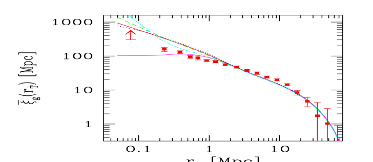
Figure 4: Projected correlation function of late-type galaxies. Data-points represent the results from Madgwick et al. (2003), while solid, dashed, dotted and dashed-dotted curves illustrate the best-fit models respectively obtained for a NFW, a power-law with $\beta=2.5$, a power-law with $\beta=2$ and a power-law with $\beta=3$ galaxy distribution profiles and for a truncation radius $r_{\rm cut}=r_{\rm vir}$. The curve flattening around $r\mathrel{\hbox to0.0pt{\lower 3.0pt\hbox{$\sim$}\hss}\raise 2.0pt\hbox{$<$}}0.5$ Mpc illustrates the contribution $\xi_{g}^{2h}$ from galaxies residing in different haloes (see text for details). The arrow shows the lower limit to the measured correlation function set on small scales by fibre collisions in the 2dF survey (Ed Hawkins, private communication).

The case for late-type galaxies appears more tricky to treat in the framework of our analysis due to the shallow slope of the observed correlation function (see Section 3.2). In fact, as it can be appreciated in Figure (4), no model can correctly describe the slow rise of the data on scales $r\mathrel{\hbox to0.0pt{\lower 3.0pt\hbox{$\sim$}\hss}\raise 2.0pt\hbox{$<$}}2$ Mpc, even though the large-scale normalization of all the curves reproduces with a good approximation the measured one. This is shown in a more quantitative way in Table 1, which quotes the minimum $\chi^{2}$ values obtained for different distribution profiles and a truncation radius $r_{\rm cut}=r_{\rm vir}$: no model gives an acceptable fit and the corresponding figures for $\chi^{2}_{min}$ are – in the best case – around 39.
A closer look at Figure (4) indicates that the problem has to be connected with the excess of power on intermediate scales exhibited by the $\xi_{g}^{2h}$ contribution of pairs of galaxies from different haloes (solid curve which flattens on scales $\sim 0.5$ Mpc), which creates the mismatch between the observed slope and the steeper “best-fit models”. In other words, what the plot reveals is that in the model there are too many pairs of galaxies coming from different haloes at distances $0.5\mathrel{\hbox to0.0pt{\lower 3.0pt\hbox{$\sim$}\hss}\raise 2.0pt\hbox{$<$}}r/[\rm Mpc]\mathrel{\hbox to0.0pt{\lower 3.0pt\hbox{$\sim$}\hss}\raise 2.0pt\hbox{$<$}}2$ with respect to what the data seem to indicate.

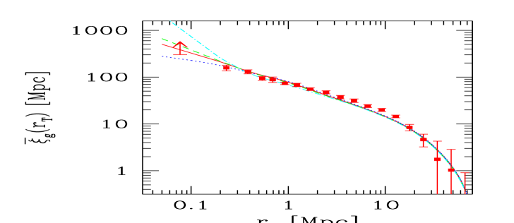
Figure 5: Projected correlation function of late-type galaxies. Data-points represent the results from Madgwick et al. (2003), while solid, dashed, dotted and dashed-dotted curves illustrate the best-fit models respectively obtained for a NFW, a power-law with $\beta=2.5$, a power-law with $\beta=2$ and a power-law with $\beta=3$ galaxy distribution profiles and for a truncation radius $r_{\rm cut}=2\cdot r_{\rm vir}$. The arrow shows the lower limit to the measured correlation function set on small scales by fibre collisions in the 2dF survey (Ed Hawkins private communication).

A possible way out is therefore to deprive the intermediate-scale region of pairs of objects residing in different haloes. This can be done if one assumes that the distribution of late-type galaxies associated to a given halo does not vanish at the virial radius, but extends to some larger distance. The mutual spatial exclusion of haloes then ensures that there will be no pairs of galaxies belonging to different haloes in the desired range. Indeed, it is not surprising to find S0 and disc galaxies futher away than a virial radius from a cluster centre (see e.g. figure 8 in Domínguez, Muriel & Lambas, 2001). We can attempt to let the galaxy distribution extend to – say – two virial radii. As Figure (5) shows, this assumption greatly reduces the discrepancy between models and measurements: the theoretical curves now have the right slope and amplitude on scales $0.5\mathrel{\hbox to0.0pt{\lower 3.0pt\hbox{$\sim$}\hss}\raise 2.0pt\hbox{$<$}}r/[\rm Mpc]\mathrel{\hbox to0.0pt{\lower 3.0pt\hbox{$\sim$}\hss}\raise 2.0pt\hbox{$<$}}2$ and the corresponding best fits to the data exhibit $\chi^{2}_{min}$ values which are (almost) as good as in the case of early-type galaxies (see Table 1). Note that, even though we adopted a somehow “ad hoc” procedure to find a better description of the measurements, our finding seems to point out to the well-known phenomenon of morphological segregation (see e.g. Madgwick et al., 2003; Domínguez, Muriel & Lambas, 2001; Giuricin et al., 2001 and Adami et al., 1998 for some recent results), whereby late-type galaxies tend to be found in the outer regions of groups and clusters, while early-type ones preferentially sink into the group or cluster centre. A simple calculation in fact shows that, for scales $0.5\mathrel{\hbox to0.0pt{\lower 3.0pt\hbox{$\sim$}\hss}\raise 2.0pt\hbox{$<$}}r/[\rm Mpc]\mathrel{\hbox to0.0pt{\lower 3.0pt\hbox{$\sim$}\hss}\raise 2.0pt\hbox{$<$}}2$, haloes which in our model are required to host star-forming galaxies up to two virial radii have masses in the range $10^{11.9}\mathrel{\hbox to0.0pt{\lower 3.0pt\hbox{$\sim$}\hss}\raise 2.0pt\hbox{$<$}}m/m_{\odot}\mathrel{\hbox to0.0pt{\lower 3.0pt\hbox{$\sim$}\hss}\raise 2.0pt\hbox{$<$}}10^{13.7}$. As we will see better in the next Section, haloes within this mass range are expected to host on average $3\mathrel{\hbox to0.0pt{\lower 3.0pt\hbox{$\sim$}\hss}\raise 2.0pt\hbox{$<$}}\langle N_{\rm gal}\rangle\mathrel{\hbox to0.0pt{\lower 3.0pt\hbox{$\sim$}\hss}\raise 2.0pt\hbox{$<$}}50$ late-type galaxies, limits which span from a small group to a cluster of galaxies.
Our result therefore does not contradict the well established fact that galaxies form within the virialized regions of dark matter haloes (i.e. at a distance $<r_{\rm vir}$ from their centre). What it simply states is that – possibly due to merging processes and accreting flows – late-type galaxies in groups and clusters are found within their dark matter haloes up to distances from the centre corresponding to about two virial radii. Note that we are not claiming that these galaxies are sling-shot towards their final position during the merging event. The key idea is that, at a certain point, in the process of approaching a merging event, galaxies residing in the progenitors of a given halo will be associated with the final object itself as their host halos loose their identity by the formation of high density “bridges” which alter the output of cluster-finding algorithms like the friends-of-friends one (on which both our mass function and bias parameters are based). This phenomenon might be less important for the population of early-type galaxies which, probably, form in galaxy mergers that tend to be more concentrated within their host haloes.

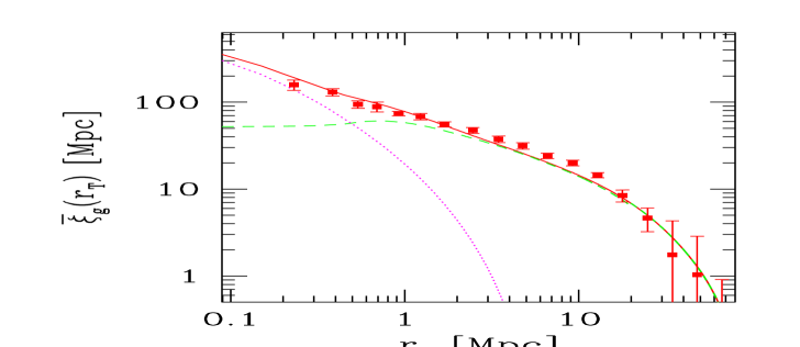
Figure 6: Projected correlation function of late-type galaxies. Data-points represent the results from Madgwick et al. (2003), while the solid curve is the best fit to the measurements obtained for a halo number density of the form (10), with $\alpha_{1}=-0.4$, $\alpha_{2}=0.7$, $m_{\rm cut}=10^{11}m_{\odot}$, $m_{0}=10^{11.4}m_{\odot}$ and for galaxies distributed within their dark matter haloes according to a NFW profile with $r_{\rm cut}=2\cdot r_{\rm vir}$. Dashed and dotted lines respectively indicate the contribution $\xi_{g}^{2h}$ from galaxies residing in different haloes and the $\xi_{g}^{1h}$ term originating from galaxies within the same halo.

We now discuss the results on the halo occupation number and distribution profile obtained for the population of late-type galaxies under the assumption of a truncation radius corresponding to two virial radii. As Table 1 shows, the best fit to the data in this case is provided by a model with $\alpha_{1}\simeq-1$, $\alpha_{2}=0.7$, $m_{\rm cut}=10^{11.1}m_{\odot}$, $m_{0}=10^{11.4}m_{\odot}$ and for galaxies distributed within their dark matter haloes according to a PL2 profile, even though on the basis of this analysis we cannot really discard any $\rho(r)$ model but PL3 since they all show $\chi_{min}^{2}$ values within 1$\sigma$ from the favourite one (as for early-type galaxies, a model is accepted as a fair description of the data if the corresponding $\chi^{2}_{min}$ lie within $\Delta\chi^{2}=3.53$ from the best fit).

In order to shed some more light on the distribution profiles able to correctly describe the correlation function of star-forming galaxies, we have then adopted the same approach as in the previous sub-section and used the lowest-$r_{\rm T}$ ($\simeq 0.07$ Mpc) measurement of $\xi_{g}(r)$ derived by the 2dF team for late-type objects (Ed Hawkins, private communication) as a lower limit to the true galaxy clustering strength, to be compared with the available models. This is done in Figure 5, where the lowest-scale data is represented by the vertical arrow. At variance with the case of early-type galaxies, the singular isothermal sphere model – even though providing the best fit to the $r\mathrel{\hbox to0.0pt{\lower 3.0pt\hbox{$\sim$}\hss}\raise 2.0pt\hbox{$>$}}0.1$ Mpc data – is now ruled out by the behaviour of the observed correlation function which in this regime needs steeper profiles. On the basis of the above comparison, one then has that only the PL2.5 a NFW density runs can still be accepted as reasonable descriptions of the data, with a slightly stronger preference given to the last model since it also provides the (second) best-fit to the observations on scales $r>0.1$ Mpc.
The projected galaxy correlation function originating from the combination of values given in Table 1 and the NFW profile is illustrated by the solid curve in Figure (6). The dashed and dotted lines respectively indicate the contribution $\xi_{g}^{2h}$ from galaxies hosted in different haloes and the $\xi_{g}^{1h}$ term given by galaxies residing within the same halo. Note that, as in Figure (2), our best-fitting models tend to underestimate the observed correlation at intermediate scales (between 5 and 15 Mpc) by $\sim 20$ per cent.

The uncertainties associated to the parameters describing the low-mass regime of the halo occupation number seem to be bigger than what found for passive galaxies. This result is however misleading, since the larger errors quoted for $\alpha_{1}$ and associated to the 1$\sigma$ lower limit of $m_{\rm cut}$ only reflect the fact that the low-mass regime in equation (10) is practically non-existent for star-forming galaxies as $m_{0}\simeq m_{\rm cut}$. In this case one than has that the halo occupation number behaves as the pure power-law: $\langle N_{\rm gal}\rangle(m)=(m/m_{0})^{\alpha_{2}}$ at almost all mass scales, where both $\alpha_{2}$ and $m_{0}$ are very well constrained.
As it was in the case of early-type galaxies, an analysis of the $\chi^{2}$ hypersurface helps understanding the interplay between the different parameters describing the halo occupation number. We find that, while $\alpha_{2}$ and $m_{0}$ show little variability, $\alpha_{1}$ and $m_{\rm cut}$ are strongly covariant, whereby higher values for the former quantity correspond to lower minimum masses associated to haloes able to host a star-forming galaxy.

As a final remark, we note that – also for late-type galaxies – values for $\alpha_{1}$, $\alpha_{2}$, $m_{\rm cut}$ and $m_{0}$ which provide the best fit to the data do not depend on the particular form adopted for the spatial distribution of galaxies within the haloes. Once again, this finding stresses the absence of degeneracy in the determination of quantities such as $\rho(r)$ and the average number of galaxies in haloes of specified mass, $\langle N_{\rm gal}\rangle(m)$: as long as one can rely on clustering measurements which probe the inner parts of dark matter haloes, both functional forms can be obtained with no degree of confusion from the same dataset.

4.3 Scatter of the Halo Occupation Distribution and Number Density Profiles

All our results for the galaxy density profiles are derived by assuming a specific functional form for $\langle N_{\rm gal}(N_{\rm gal}-1)\rangle(m)$, as given in equation (13). In principle, this could bias our determination of the spatial distribution of galaxies within a single halo (Berlind & Weinberg 2002). In order to understand the importance of this effect, we repeated the analysis of the correlation functions by assuming 3 different functional forms for the second moment of the halo distribution function. In particular, we took $\alpha=1,0.3,0.1$ in equation (13) independently of the halo mass. We found that none of these models can fit the data as well as our original prescription. However, for purely Poissonian scatter, the best-fitting models for late-type galaxies are almost identical to our fiducial models, and the ranking of the density profiles does not change. On the other hand, for early-type galaxies, Poissonian models are associated with large values of $\chi^{2}$ (23.7 at best, for PL2) due to the overabundance of power on small scales (the favorite values for $m_{\rm cut}$ and $m_{0}$ tipically are $\sim 10$ times smaller than in our fiducial case) but, still, only the PL2 and NFW profiles are acceptable. When the scatter, instead, is strongly sub-Poissonian ($\alpha=0.1,0.3$) we find that it is practically impossible to get a good description of $\bar{\xi}_{g}$. In fact, in this case, the 1-halo term in the correlation function is heavily depressed and one is forced to increase the value of $\alpha_{2}$ and $m_{\rm cut}$ to try to match the data. Anyway, all the models are unacceptable due to lack of power on small scales, and all the profiles are associated with nearly the same values of $\chi^{2}$. In summary, even though we confirm the presence of some degeneracy between the second moment of the halo occupation distribution and the profile of the galaxy distribution as discussed in Berlind & Weinberg (2002), we found that it is extremely hard to find models that can give accurate description of the data. This means that the apparent freedom in assuming a functional form for $\langle N_{\rm gal}(N_{\rm gal}-1)\rangle(m)$ is not such. As a consequence of this, we are led to believe that our conclusions regarding the density profiles of 2dF galaxies are indicative of a real trend, even though they are indeed drawn in the framework of a specific model.

5 The Galaxy Mass Function

The results derived in the previous sections allow us to draw some conclusions on the intrinsic nature of galaxies of different types. Figure (7) shows the average number of galaxies per dark matter halo of specified mass $m$ as obtained from the best fits to the clustering measurements of Madgwick et al. (2003). The dashed line describes the case for star-forming galaxies, while the solid line is for early-type objects.

Late-type galaxies are found in haloes with masses greater than $\sim 10^{11}\;m_{\odot}$ (even though this figure, especially in its lower limit, is not determined with a great accuracy given the interplay between $m_{\rm cut}$ and $\alpha_{1}$), and their number increases with the mass of the halo which hosts them according to a power-law (except in the limited region $10^{11.0}\leq m/m_{\odot}<10^{11.4}$) with slope $\alpha_{2}=0.7$ and normalization $1/m_{0}=10^{-11.4}m_{\odot}^{-1}$.
Early-type galaxies instead start appearing within haloes of noticeably higher masses, $m\mathrel{\hbox to0.0pt{\lower 3.0pt\hbox{$\sim$}\hss}\raise 2.0pt\hbox{$>$}}10^{12.6}\;m_{\odot}$. In the low-mass region (i.e. for $m\mathrel{\hbox to0.0pt{\lower 3.0pt\hbox{$\sim$}\hss}\raise 2.0pt\hbox{$<$}}10^{13.5}\;m_{\odot}$), the data seems to indicate that each halo is on average populated by approximately one passive galaxy, even though results in this mass range are affected by some uncertainties. More solid are the findings in the high mass ($m\mathrel{\hbox to0.0pt{\lower 3.0pt\hbox{$\sim$}\hss}\raise 2.0pt\hbox{$>$}}10^{13.5}\;m_{\odot}$) regime, which show $\langle N_{\rm gal}\rangle$ to increase with halo mass as a power-law of slope $\alpha_{2}\simeq 1.1$, steeper than what found for the population of late-type galaxies. One then has that the average number of star-forming galaxies within a halo does not increase with its mass as fast as it happens for passive galaxies, even though late-type objects are found to dominate the 2dF counts at all mass scales. This result seems in disagreement with the observational evidence that early-type galaxies are preferentially found in clusters, while star-forming galaxies mainly reside in relatively underdense regions. The discrepancy is however only apparent since, while in the Madgwick et al. (2003) analysis the population of early-type galaxies is an homogeneous sample, the class of late-type galaxies includes any object which has some hint of star-formation activity in its spectrum (see Section 3). This implies that anything – from highly irregular and star-bursting galaxies to S0 types – will be part of the star-forming sample. The lack of a characteristic mass for the transition from haloes mainly populated by late-type galaxies to haloes principally inhabited by passive objects then finds a natural explanation if one considers that S0 galaxies – also preferentially found in groups and clusters – are in this case associated to the population of late-type objects, making up for about 35 per cent of the sample (Madgwick et al., 2002). We also remind that both the 2dF and its parent APM surveys select sources in the blue ($b_{j}$) band, therefore creating a bias in favour of star-forming galaxies which are more visible than passively evolving ellipticals in this wavelength range.

It is interesting to compare our results with those by van den Bosch et al. (2003) who used 2dF data to estimate the conditional luminosity functions of early- and late-type galaxies. They combined their results to obtain the mean halo occupation number of galaxies in given absolute-magnitude ranges. Since our analysis is based on a apparent-magnitude limited sample, this complicates the comparison. For their faintest late-type galaxies, the behaviour of $\langle N_{\rm gal}\rangle(m)$ is relatively similar to our findings with a cutoff below $\sim 10^{11}m_{\odot}$, a small decrement up to $10^{11.5}m_{\odot}$ and a power-law regime $d\log\langle N_{\rm gal}\rangle(m)/d\log m\simeq 0.6$ for larger masses. As for early-type galaxies, results are in good agreement, with a power-law high-mass regime with slope $d\log\langle N_{\rm gal}\rangle(m)/d\log m\simeq 1$. However, van den Bosch et al. (2003) find a less sharp cutoff at small masses, with $\log(m_{0}/m_{\odot})\sim 12.5$ and $\langle N_{\rm gal}(m)\rangle$ gently declining with decreasing $m$ till to $10^{10.5-11}m_{\odot}$. Given all the systematic uncertainties belonging to the two method of analysis the similarity of the results is remarkable, confirming the potential of the halo occupation distribution method.

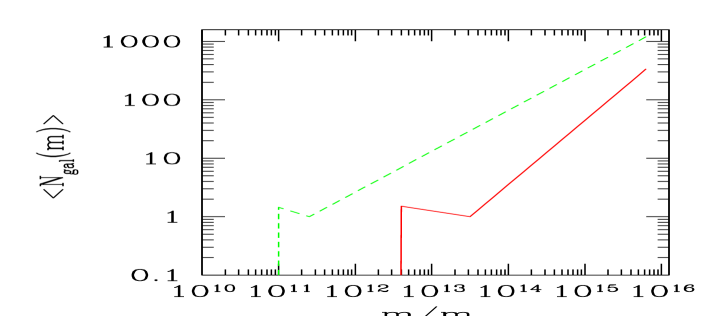
Figure 7: Average number of galaxies $\langle N_{\rm gal}(m)\rangle$ per dark matter halo of specified mass $m$ (expressed in $m_{\odot}$ units). The solid line represents the case for early-type galaxies, while the dashed line is for late-type objects.

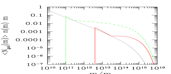
Figure 8: Number of galaxies per unit of (log) dark matter mass and volume (in ${\rm Mpc}^{-3}$ units). The solid line represents the result for early-type galaxies, while the dashed line is for late-type objects. For comparison, the dotted line indicates the Sheth & Tormen (1999) mass function $n(m)$ of dark matter haloes.

Finally, Figure (8) shows the “galaxy mass function” i.e. the number density of galaxies per unit of dark matter mass and volume as obtained by multiplying the average number of galaxies found in a halo of specified mass $\langle N_{\rm gal}(m)\rangle$ by the halo mass function (10). Again, the solid curve identifies the case for early-type galaxies, while the dashed one is derived for the population of star-forming galaxies. The dotted line indicates the Sheth & Tormen (1999) halo mass function (10).

6 Conclusions

Results from Madgwick et al. (2002) and (2003) on the correlation function and luminosity function of $\sim 96,000$ 2dFGRS galaxies with $0.01<z<0.15$ have been used to investigate some of the properties of early- and late-type galaxies, such as the so-called halo occupation number $\langle N_{\rm gal}\rangle$ (i.e. the mean number of sources that populate a halo of given mass $m$) and the spatial distribution of such galaxies within their dark matter haloes.

In order to perform our analysis, we have considered four distribution profiles: three power-laws of the form $\rho(r)\propto r^{-\beta}$ with $\beta=2,2.5,3$ and a NFW profile chosen to mimic the assumption for galaxies within haloes to trace the distribution of dark matter. As a first approximation, all the profiles have been truncated at the halo virial radius.
For consistency with results from semi-analytical models (see e.g. Benson et al., 2001), the halo occupation number was parametrized by a broken power-law of the form $(m/m_{0})^{\alpha_{1}}$ in the low mass regime $m_{\rm cut}\leq m\leq m_{0}$ and $(m/m_{0})^{\alpha_{2}}$ at higher masses, where $m_{\rm cut}$ is the minimum mass of a halo that can host a galaxy.

The resulting theoretical average number density $\bar{n}_{g}$ and galaxy-galaxy correlation function – sum of the two terms $\xi_{g}^{1h}$, representing the contribution from galaxies residing within the same halo, and $\xi_{g}^{2h}$ which considers pairs belonging to different haloes – have then been compared with the observations in order to determine those models which provide the best description of the data both in the case of late-type and early-type galaxies. Note that, at variance with previous works which only considered a linear $\xi_{g}^{2h}$, our analysis provides a full treatment for non-linearity and also includes the assumption of halo-halo spatial exclusion, in a way that makes the model entirely self-consistent.

The main conclusions are as follows:

1. Early-type galaxies are well described by a halo occupation number of the form broken power-law (10) with $\alpha_{1}\simeq-0.2$, $\alpha_{2}\simeq 1.1$, $m_{\rm cut}\simeq 10^{12.6}m_{\odot}$ and $m_{0}\simeq 10^{13.5}m_{\odot}$, where the two quantities which determine the intermediate-to-high mass behaviour of $\langle N_{\rm gal}\rangle$ are measured with a good accuracy.

2. No model can provide a reasonable fit to the correlation function of late-type galaxies since they all show an excess of power with respect to the data on scales $0.5\mathrel{\hbox to0.0pt{\lower 3.0pt\hbox{$\sim$}\hss}\raise 2.0pt\hbox{$<$}}r/[\rm Mpc]\mathrel{\hbox to0.0pt{\lower 3.0pt\hbox{$\sim$}\hss}\raise 2.0pt\hbox{$<$}}2$. In order to obtain an acceptable description of the observations, one has to assume that star-forming galaxies are distributed within haloes of masses comparable to those of groups and clusters up to two virial radii. This result is consistent with the phenomenon of morphological segregation whereby late-type galaxies are mostly found in the outer regions of groups or clusters (extending well beyond their virial radii), while passive objects preferentially sink into their centres.

3. With the above result in mind, one finds that late-type galaxies can be described by a halo occupation number of the form single power-law with $\alpha_{2}\simeq 0.7$, $m_{\rm cut}\simeq 10^{11}m_{\odot}$ and $m_{0}\simeq 10^{11.4}m_{\odot}$, where the quantities which describe $\langle N_{\rm gal}\rangle$ in the high-mass regime are determined with a high degree of accuracy.

4. Within the framework of our models, galaxies of any kind seem to follow the underlying distribution of dark matter within haloes as they present the same degree of spatial concentration. In fact the data indicates both early-type and late-type galaxies to be distributed within their host haloes according to NFW profiles. We note however that, even though early-type galaxies can also be described by means of a shallower distribution of the form $\rho(r)\propto r^{-2}$, this cannot be accepted as a fair modelling of the data in the case of late-type galaxies which instead allow for somehow steeper ($\beta\simeq 2.5)$ profiles. In no case a $\beta=3$ density run can provide an acceptable description of the observed correlation function. These conclusions depend somehow on assuming a specific functional form for the second moment of the halo occupation distribution. We showed, however, that there is not much freedom in the choice of this function is one wants to accurately match the observational data.

An interesting point to note is that results on the spatial distribution of galaxies within haloes and on their halo occupation number are independent from each other. There is no degeneracy in the determination of $\langle N_{\rm gal}\rangle$ and $\rho(r)$ as they dominate the behaviour of the two-point correlation function $\xi_{g}$ at different scales. Different distribution profiles in fact principally determine the slope of $\xi_{g}$ on small enough ($r\mathrel{\hbox to0.0pt{\lower 3.0pt\hbox{$\sim$}\hss}\raise 2.0pt\hbox{$<$}}1$ Mpc) scales which probe the inner regions of the haloes, while the halo occupation number is mainly responsible for the overall normalization of $\xi_{g}$ and for its slope on large-to-intermediate scales.

Our analysis shows that late-type galaxies can be hosted in haloes with masses smaller than it is the case for early-type objects. This is probably due to the fact that early-type galaxies are on average more massive (where the term here refers to stellar mass) than star-forming objects, especially if one considers the population of irregulars, and points to a relationship between stellar mass of galaxies and mass of the dark matter haloes which host them.

The population of star-forming galaxies is found to be the dominant one at all mass scales, result that can be reconciliated with the well established observational fact that early-type galaxies are preferentially found in clusters, while star-forming galaxies mainly reside in relatively underdense regions, by considering that about a third of the class of late-type sources in our sample is made of S0 galaxies, which are also preferentially found in groups and clusters. We also stress that both the 2dF and its parent APM surveys select sources in the blue band, therefore creating a bias in favour of star-forming galaxies which are more visible than passively evolving ellipticals in this wavelength range.

As a final remark, we note that the results of this work are partially biased by the need to assume a pre-defined functional form for both the halo occupation number and the variance about this quantity. High precision measurements of higher moments of the galaxy distribution function (such e.g. the skewness and the kurtosis) are of crucial importance if one wants to determine the distribution of galaxies within dark matter haloes in a non-parametric way, i.e. without the necessity to rely on any “a priori” assumption. In the near future, results from the 2dF and SSDS galaxy redshift surveys should be able to fill this gap.

References

- [Adami1998] Adami C., Biviano A., Mazure A., 1998, A&A, 331, 439
- [Ben12001] Benson A.J., 2001, MNRAS, 325, 1039
- [Ben2001] Benson A.J., Cole S., Frenk C.S., Baugh C.M., Lacey C.G., 2001, 327, 1041
- [Berlind2002] Berlind A.A., Weinberg D.H., 2002, ApJ, 575, 587
- [Berletal2003] Berlind A.A. et al., 2003, Ap.J., in press, astro-ph/0212357
- [Bullock-22002] Bullock J.S., Wechsler R. H. & Somerville, R.S., 2002, MNRAS, 329, 246
- [Bullock2001] Bullock J.S., Kolatt T.S., Sigad, Y., Somerville R.S., Kravtsov A.V., Klypin A.A., Primack J.R., Dekel A., 2001, ApJ, 321, 559
- [Cate1998] Catelan P., Lucchin F., Matarrese S. & Porciani C., 1997, MNRAS, 297, 692
- [CK 1989] Cole S. & Kaiser N., 1989, MNRAS, 237, 1127
- [Colless 2001] Colless M. et al. (2dFGRS team), 2001, MNRAS, 328, 1039
- [Cooray 2002] Cooray A., Sheth R., 2002, astro-ph/0206508
- [Diaferio1999] Diaferio A., Kauffmann G., Colberg J.M., White S.D.M., 1999, MNRAS, 307, 537
- [dom01 2001] Domínguez M., Muriel H., Lambas D.G., 2001, ApJ, 121, 1266
- [Folkes et al. 1999] Folkes S.R., Ronen S., Price I., Lahav O., Colless M., Maddox S.J., Glazebrook K., Bland-Hawthorn J, Cannon R., Cole S., Collins C., Couch W., Driver S., Dalton G., Efstathiou G., Ellis R., Frenk C., Kaiser N., Lewis L., Lumsden S., Peacock J., Peterson B., Sutherland W., Taylor K., 1999, MNRAS, 308, 459.
- [Gatz1995] Gaztanaga E., 1995, MNRAS, 454, 561
- [Giu2001] Giuricin G., Samurovic S., Girardi M., Mezzetti M., Marinoni C., 2001, ApJ, 554, 857
- [guzzo1997] Guzzo L., Strauss M.A., Fisher K.B., Giavanelli R., Haynes M.P., 1997, ApJ, 489, 37
- [Hawkins2002] Hawkins E., et al. (the 2dFGRS Team), 2003, MNRAS, submitted, (astro-ph/0212375)
- [Jenkins1998] Jenkins A., et al. (the VIRGO Consortium), 1998, ApJ, 499, 20
- [Jen012001] Jenkins A., Frenk C.S., White S.D.M., Colberg J.M., Cole S., Evrard A.E., Couchman H.M.P. & Yoshida N., 2001, MNRAS, 321, 372
- [Lahav2002] Lahav O., et al. (2dFGRS Team), 2002, MNRAS, 333, 961
- [Lin1996] Lin H., Kirshner R.P., Shectman S.A., Landy S.D., Oemler A., Tucker D.L., Schechter P.L., 1996, ApJ, 464,60
- [lov11995] Loveday J., Maddox S.J., Efstathiou G., Peterson B.A., 1995, ApJ, 442 457
- [lov21999] Loveday J., Tresse L., Maddox S.J., 1999, MNRAS, 310, 281
- [Maddox et al. 1990a] Maddox S.J., Efstathiou G., Sutherland W.J., Loveday J., 1990a, MNRAS, 243, 692
- [Maddox et al. 1990b] Maddox S.J., Efstathiou G., Sutherland W.J., 1990b, MNRAS, 246, 433
- [Maddox et al. 1996] Maddox S.J., Efstathiou G., Sutherland W.J., 1996, MNRAS, 283, 1227
- [Madgwick12002] Madgwick D.S., et al. (the 2dFGRS Team), 2002, MNRAS, 333, 133
- [Madgwick22002] Madgwick D.S., et al. (the 2dFGRS Team), 2003, MNRAS, submitted (astro-ph/0303668)
- [Maglio2000] Magliocchetti M., Bagla J., Maddox S.J., Lahav O., 2000, MNRAS, 314, 546
- [maglio1 2001] Magliocchetti M., Moscardini L., Panuzzo P., Granato G.L., De Zotti G., Danese L., 2001, MNRAS, 325, 1553
- [marinoni 2001] Marinoni C. & Hudson M.J., 2002, ApJ, 569, 101
- [martini 2001] Martini P. & Weinberg D.H., 2001, ApJ, 547, 12
- [Matarrese1997] Matarrese S., Coles P., Lucchin F., Moscardini L., 1997, MNRAS, 286, 115
- [Mo1996] Mo H.J., White S.D.M., 1996, MNRAS, 282, 347
- [Moscardini1998] Moscardini L., Coles P., Lucchin F., Matarrese S., 1998, MNRAS, 299, 95
- [mou 2002] Moustakas L., Somerville R.S., 2002, ApJ, 577, 1
- [NFW1997] Navarro J.F., Frenk C.S., White S.D.M., 1997, ApJ, 490, 493
- [Norberg2002] Norberg P., et al. (the 2dFGRS Team), 2002, MNRAS, submitted, astro-ph/0112043
- [Peacock 1996] Peacock J.A. & Dodds S.J., 1996, MNRAS, 267, 1020
- [Peacock3 2000] Peacock J.A. & Smith R.E., 2000, MNRAS, 318, 1144
- [Porci 2002] Porciani C., Giavalisco M., 2002, ApJ, 565, 24
- [Porcietal 1998] Porciani C., Matarrese S., Lucchin F. & Catelan P., 1998, MNRAS, 298, 1097
- [Scher1991] Scherrer R.J., Bertschinger E., 1991, ApJ, 381, 349
- [Scocci2001] Scoccimarro R., Sheth R.K., Hui L.,Jain B., 2001, ApJ, 546, 20
- [sel 2000] Seljak U., 2000, MNRAS, 318, 203
- [sheth 1999] Sheth R.K., Tormen G., 1999, MNRAS, 308, 119
- [sheth1 2001] Sheth R.K., Diaferio A., 2001, MNRAS, 322, 901
- [sheth2 2001] Sheth R.K., Mo H.J. & Tormen G., 2001, MNRAS, 323, 1
- [som2001] Somerville R.S., Lemson G., Sigad Y., Dekel A., Kauffmann G., White S.D.M., 2001, MNRAS, 320, 289
- [spe2003] Spergel D.M., et al., 2003, astro-ph/0302209
- [vdb2003] van den Bosch F.C., Yang X., Mo H.J., 2003, MNRAS, 340, 771
- [vdb2003] van den Bosch F.C., Mo H.J., Yang X., 2003, astro-ph/0301104
- [ymv2003] Yang X., Mo H.J., van den Bosch F.C., 2003, MNRAS, 339, 1057
- [yan2003] Yang X., Mo H.J., Jing Y.P., van den Bosch F.C., Chu Y., 2003, MNRAS, submitted, astro-ph/0303524
- [York 2000] York D.G., Anderson J.E., Anderson S.F., Annis J., Bachall N.A., Bakken J.A., et al., 2000, AJ, 120, 1579
- [Zehavi 2003] Zehavi et al. (the SDSS Collaboration), 2003, astro-ph/0301280