Mapping the expansion of the universe gives clues to the underlying physics causing the recently discovered acceleration of the expansion, and enables discrimination among cosmological models. We examine the utility of measuring the rate of expansion, $H(z)$, at various epochs, both alone and in combination with distance measurements. Due to parameter degeneracies, it proves most useful as a complement to precision distance-redshift data. Using the baryon oscillations in the matter power spectrum as a standard rod allows determination of $H(z)/(\Omega_{m}h^{2})^{1/2}$ free of most major systematics, and thus provides a window on dark energy properties. We discuss the addition of this data from a next generation galaxy redshift survey such as KAOS to precision distance information from a next generation supernova survey such as SNAP. This can provide useful crosschecks as well as lead to improvement on estimation of a time variation in the dark energy equation of state by factors ranging from 15-50%.

1 Introduction

We now have strong evidence that the expansion of the universe is accelerating, from the original method of Type Ia supernova distance-redshift measurements [1, 2] and concordant observations of the cosmic microwave background (CMB) power spectrum and of large scale structure [3, 4]. The nature of the dark energy responsible for the acceleration will have profound implications for cosmology, particle physics, and fundamental physics. Mapping the expansion history of the universe offers a way to gain insights into the dark energy and the fate of the universe, for example by characterizing the equation of state behavior that is directly related to properties of the scalar field potential.

As discussed in Linder [5], one would like to carry out this mapping with not only precision measurements of the distance-redshift relation, but ideally with data on differential distances corresponding to the change between neighboring redshift epochs. The former, notably from the Type Ia supernova method, have proved adept at constraining the energy density and equation of state of the dark energy, with great improvements expected in the next decade. But these involve an integration over the expansion rate behavior $H(z)$, which itself involves a redshift integral over the equation of state $w(z)$. Probes more closely related to the differential distance might give $H(z)$ more directly.

However the integral nature of the distance-redshift relation also provides the power to break degeneracies between cosmological parameters, which is an equally important aspect. So [5] found that the Alcock-Paczyǹski effect of the cosmic shear distortion – due to the source distances radial and transverse to the line of sight being measured at different epochs – did not in fact automatically give more stringent estimations of the dark energy properties, despite involving a bare factor $H(z)$. The cosmic shear (not to be confused with the local, weak lensing shear) is related to the ratio of the differential distance over some redshift interval to the integrated distance to the source. So it is interesting to consider whether the situation changes if we can independently measure the two quantities, basically finding the Hubble parameter $H(z)$ separately.

In Section 2 we investigate the use of $H(z)$ for constraining the cosmological model. But in Section 3 we find that the most promising technique – the baryon oscillation method – actually measures a slightly different quantity. We then examine the use of the radial and transverse distances provided by precision next generation galaxy redshift survey observations of the linear matter power spectrum, separately and together. In Section 4 we show that the full power of the method comes from adding the information to a deep distance survey such as from accurate observations of Type Ia supernovae (e.g. SNAP). We summarize our conclusions and the need for future work in Section 5.

2 Using $H(z)$ Information

In this section we consider a data set giving the Hubble parameter $H(z)$ at some redshifts $z$, with a certain fractional precision. This is a purely theoretical investigation as we do not specify how the measurements are made. Indeed, as mentioned in the introduction, the cosmic shear method only gives the product of $H(z)$ with the distance corresponding to the redshift $z$, and as we will see in §3 the baryon oscillation method also provides a ratio involving $H(z)$. So this is meant as a thought experiment.

Similarly, it is obvious that knowledge of $H(z)$ over the entire redshift range from the observer at $z=0$ out to some depth is overly optimistic and would supersede any distance measurements in that range. So we consider data at only a few redshifts in a narrow range and ask what cosmological information this can provide and what value it adds to a more realistic set of distance measurements. Recall that the comoving distance $r$ or conformal time $\eta$ is related to $H(z)$ in a flat universe by

$$r(z)=\eta(z)=\int_{0}^{z}dz^{\prime}\,H^{-1}(z^{\prime}),$$ (1)

and the angular diameter distance $d_{a}=(1+z)^{-1}r$ and luminosity distance $d_{l}=(1+z)\,r$. The differential distance along the line of sight (radially) is simply $dr_{\parallel}=d\eta=dz/H$ and transversely is $dr_{\perp}=\eta\theta$, where $\theta$ is the angle subtended.

Through the Friedmann equations, the expansion rate $H(z)$ is related to the cosmological components by

$$(H/H_{0})^{2}=\Omega_{m}(1+z)^{3}+(1-\Omega_{m})e^{3\int_{0}^{z}d\ln(1+z^{\prime})\,[1+w(z^{\prime})]},$$ (2)

where $H_{0}$ is the Hubble constant, the present value $H(z=0)$, $\Omega_{m}$ is the dimensionless matter density, and $w(z)$ is the equation of state of the dark energy. We can examine the impact of measurements of $H(z)$ on determinations of the cosmological parameters through the sensitivities $\partial H/\partial\Omega_{m}$ etc., achieving formal constraints through the Fisher matrix method [6].

The sensitivities are shown in Figure 1, with the parametrization $w(z)=w_{0}+w_{a}z/(1+z)$ of Linder [7] that allows robust treatment of the equation of state to redshifts greater than one. However, the sensitivities are not the whole story: degeneracies between the parameters play a major role in determining them. For example, while a 1% measurement of $H(z)$ at $z=3$, say, would apparently constrain $\Omega_{m}$ to 0.06, $w_{0}$ to 0.14, and $w_{a}$ to 0.3, this holds only upon fixing all parameters but one. In fact a measurement at a single redshift only gives an infinite ellipsoid in the joint three dimensional parameter space. Even over a redshift range, such as $H(z)$ to 1% at $z=2.8$, 3, 3.2, the uncertainties are uselessly large: $\sigma(\Omega_{m})=0.87$, $\sigma(w_{0})=76$, $\sigma(w_{a})=207$. But because the ellipsoid is fairly narrow, and the degeneracy direction is different than for distance measurements, the combination of $H(z)$ information with distance information can be valuable.

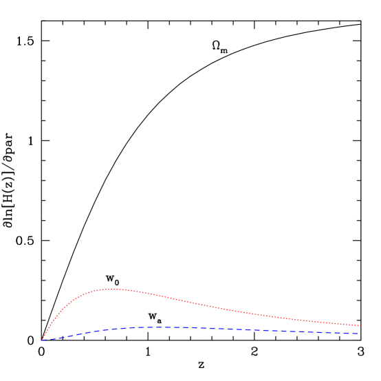
Figure 1: The sensitivity of the expansion rate $H(z)$ to the cosmological parameters is plotted as a function of redshift. The larger the derivative at a particular redshift, the more constraining the observations are there, but the curves by themselves do not account for degeneracies between the parameters.

For example, adding the estimation of $H(z)$ at $z=2.8$, 3, 3.2 to a simulation of the data expected from the Supernova/Acceleration Probe (SNAP; [8]) survey out to $z=1.7$ allows parameter determination to $\sigma(\Omega_{m})=0.0082$, $\sigma(w_{0})=0.078$, $\sigma(w_{a})=0.45$. This represents a factor 3.5 improvement in constraining $\Omega_{m}$, 2% in $w_{0}$, and 23% in the measure of the time variation $w^{\prime}\approx w_{a}/2$, relative to the canonical SNAP results. So as expected there is clearly value in obtaining measurements of $H(z)$ (though we have not established how such would be carried out) – though only in complementarity with a distance probe.

Indeed one can show that measurements of $H(z)$ at redshifts $z>1$ basically act like information about the matter density $\Omega_{m}$. If one eschewed any $H(z)$ data but added a prior $\sigma_{\Omega_{m}}=0.0082$ to the SNAP data then one would roughly recover the previous parameter estimations. This is not surprising since at $z>1$ one is increasingly in the matter dominated, deceleration epoch and the expansion rate therefore best measures the matter density, not the dark energy properties. So an integral measure such as the distance-redshift relation actually has an advantage in probing the dark energy equation of state, despite this quantity entering the distance through a double integral.

We emphasize this important point further by considering two elaborations. If we spread the redshift range of the $H(z)$ measurements, to $z=2.5$, 3, 3.5 and add simulated information from the future Planck cosmic microwave background survey [9], then the dark energy constraints are still weak: $\sigma(\Omega_{m})=0.039$, $\sigma(w_{0})=1.6$, $\sigma(w_{a})=5.4$. Again, the CMB has limited sensitivity to the dark energy equation of state and little complementarity with the $H(z)$ measurement. If we now add the SNAP data, the estimations improve to 0.0056, 0.070, and 0.34 respectively, but little of this is due to $H(z)$ since the CMB complementarity is much stronger. The part of the improvement due to $H(z)$ is mostly restricted to $\Omega_{m}$ (since that is what $H(z=3)$ best probes) and somewhat $w_{0}$ (due to its degeneracy with $\Omega_{m}$); adding $H(z)$ tightens estimation of $\Omega_{m}$ by 44%, $w_{0}$ by 11%, but $w_{a}$ by only 4%.

For determination of $H(z)$ near $z=1$, the situation is only slightly better. It no longer acts as predominantly a matter density prior, but again $H(z)$ by itself cannot constrain the dark energy parameters, even with observations over a range $z=0.5-1.5$. Furthermore, it has less complementarity with SNAP data and improves $w_{a}$ constraints by only 6%. But conversely it gains in complementarity with the CMB information, and improves SNAP+CMB parameter determinations of $\Omega_{m}$, $w_{0}$, $w_{a}$ by 12%, 23%, 16% respectively. These various cases are illustrated in Fig. 2.

So the distance data plays a central role in determining dark energy properties and $H(z)$ measurements only a subsidiary, complementary one. But in any case we note that we have not identified any cosmological probe that provides these Hubble parameter measurements, let alone at 1% accuracy.

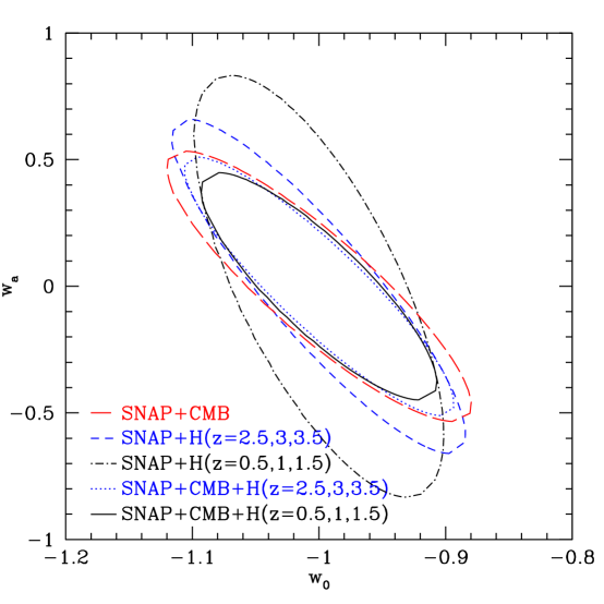
Figure 2: Joint probability contours (68% confidence level) for the time variation $w_{a}$ and the present value $w_{0}$ of the dark energy equation of state show that measurement of $H(z)$ is not as powerful as the CMB in complementing supernova data.

3 Baryon Oscillations

One cosmological probe that shows promise in obtaining differential distance measurements is the use of the imprint of the primordial baryon-photon acoustic oscillations in the matter power spectrum. These are analogous to the oscillations appearing in the CMB temperature power spectrum, but are much smaller, appearing as wiggles superposed on the larger dark matter component (see [10, 11] for a comprehensive discussion). The wiggle wavelength can be used as a standard ruler, since the intrinsic scale is known from well understood physics of the matter-radiation decoupling epoch. Then the angular or redshift space scale can be measured through a wide field redshift survey (though beyond the current state of the art) and the comparison probes the cosmological model.

By observing at redshifts $z>1$ some of the wiggles appear in the linear density regime of the power spectrum, and by using only the locations and not the amplitudes of the oscillations one does not require problematic models of structure formation and evolution. This method then has several positive aspects: simple, linear physics free from astrophysical uncertainties, direct relation of observations to cosmological quantities, and sensitivity to a snapshot of the expansion rate, $H(z)$. For further discussion of the details and possible implementation of this probe see [12, 13, 14].

However, the baryon oscillations do not provide a pure measure of $H(z)$. Rather, the physics involves the ratio of the “standard rod” size to the observed oscillation scale (generally in Fourier wavenumber, $k$-space). So the central quantity is

$$K\equiv{k_{A}\over k_{obs}}={1\over s}dz{d\eta\over dz}={dz\over H(z)\,s},$$ (3)

where $k_{A}$ is the predicted acoustic oscillation scale, proportional to the inverse of the sound horizon $s$, and $k_{obs}$ is the observed scale, proportional to the inverse of the standard rod length $d\eta$. The sound horizon is given by

$$s = \int_{z_{dec}}^{\infty}dz\,(c_{s}/H)$$ (4)

$$= (\Omega_{m}h^{2})^{-1/2}\int da\,c_{s}\,\Bigr{[}a+a_{eq}+(1-\Omega_{m}^{-1})a^{4}e^{-3\int d\ln a\,[1+w(a)]}\Bigl{]}^{-1/2},$$ (5)

where $a=(1+z)^{-1}$ is the scale factor of the universe, $c_{s}$ is the sound speed in the baryon fluid, $z_{dec}$ is the redshift of decoupling, and $a_{eq}$ is the scale factor at matter-radiation equality. Note that while a cosmological constant ($w=-1$) would cause the last term in the brackets to have a negligible contribution to the integrand, some forms of dynamical dark matter could have non-negligible influence at these redshifts (see [15] for a discussion of early quintessence). The sound speed for adiabatic perturbations in the baryons is

$$c_{s}={1\over\sqrt{3}}\left(1+{3\over 4}{\rho_{b}\over\rho_{\gamma}}\right)^{-1/2}.$$ (6)

Since the baryon density $\rho_{b}\sim\Omega_{b}h^{2}$ is well determined by current CMB measurements, and will be further improved by Planck data, and the photon density $\rho_{\gamma}\sim T_{\gamma}^{4}$ is also accurately known, then we can regard $c_{s}$ as fixed.

From the form of Eqs. (3) and (4), we see that $H(z)$ enters in both numerator and denominator, as itself and as an integrand. This is the same form as for the cosmic shear probe [5]. So as pointed out there, the value of the Hubble constant $H_{0}$ or $h$ does not enter the problem and therefore does not require marginalization. This is a definite advantage. Furthermore, one can divide numerator and denominator by $(\Omega_{m}h^{2})^{1/2}$. At a casual glance, one might think that all dependence on this quantity is then removed. But in fact, the approximation that $s\sim(\Omega_{m}h^{2})^{-1/2}$ is not a good one, as pointed out in [16]. There, a closer approximation for a flat, cosmological constant universe was found to be $s\sim(\Omega_{m}h^{2})^{-0.3}$, while a more precise analysis [11] is equivalent to $s\sim(\Omega_{m}h^{2})^{-0.23}$. The additional factors come from the presence of $a_{eq}$ and to a much lesser extent $a_{dec}$. However, since the dependence arises from the sound horizon, it is the same for all the redshifts at which the measurements of $k_{obs}$ are carried out by the redshift survey. This, combined with the precision to which Planck will determine $\Omega_{m}h^{2}$, means that its uncertainty couples very weakly to the other parameters (this was explicitly tested), and we will neglect it. However, one still must incorporate the uncertainty in $\Omega_{m}$ in order to obtain realistic parameter error estimations.

Therefore, the baryon oscillation method can essentially provide measurements of two cosmological variables according to Eq. (3): $\tilde{H}(z)\equiv H(z)/(\Omega_{m}h^{2})^{1/2}$ and $\tilde{\eta}(z)\equiv r(z)\,(\Omega_{m}h^{2})^{1/2}$. These come respectively from the wavenumbers along ($d\eta$) and transverse ($\eta$) to the line of sight. This distinction from a plain $H(z)$ as treated in §2 is important for the parameter degeneracies and complementarity with other methods.

Figure 3 shows the sensitivities for these two quantities. As expected, for $w_{0}$ and $w_{a}$ the derivatives are the same as for $H(z)$ and $r(z)$. However, the degeneracy relations between the parameters have now changed, and so the strength of the estimations have as well. Again we find that the probe in isolation cannot effectively constrain the cosmological model – even the matter density since most of its dependence has been removed in the ratio. Even in combination with CMB data it has little leverage.

However the situation changes significantly for a fiducial model that has time variation in the equation of state. For a supergravity inspired model [17] that is well fit by $w_{0}=-0.82$, $w_{a}=0.58$, the oscillation data offers definite sensitivity to the time variation. Now a 2% (1%) measurement of $K$ in both its radial and transverse aspects, in combination with Planck data, allows estimation of $w_{a}$ to 0.29 (0.20) for measurements at $z=\{0.5,1,1.5\}$ and 0.62 (0.47) for $z=\{2.5,3,3.5\}$. However, the estimations of $w_{0}$ remain poor: 0.16 (0.09) and 0.36 (0.27) respectively. Furthermore, since only 1-2 wiggles are in the linear regime at $z\approx 1$, the observations are unlikely to achieve better than 2% precision there, while we see that even 1% precision at $z\approx 3$ gives less impressive results. And of course we have no guarantee that the true cosmological model will have a strong time variation in the dark energy equation of state.

Figure 3: As Fig. 1 but for the baryon oscillation scale. Baryon oscillation measurements provide two quantities, corresponding to wave modes along [$d\eta$] and transverse [$\eta$] to the line of sight. The $\Omega_{m}$ curves do not have zero sensitivity at $z=0$ because of the division by $(\Omega_{m}h^{2})^{1/2}$.

4 Baryon Oscillations Plus Supernovae

As with the $H(z)$ analysis in §2, the baryon oscillation method cannot stand alone as a robust cosmological probe. In this section we consider it in complement with a SNAP supernova distance survey. As expected, we find that it does not behave in the same manner as $H(z)$, as effectively a prior on the matter density. In fact, unlike $H(z)$, within a cosmological constant model of dark energy the complementarity with precision distance measurements is now substantial, providing good constraints. Adding oscillation information acts even slightly more strongly than adding CMB information, relative to supernovae. When the baryon oscillation information is added to SNAP+CMB, further modest improvements are seen – around 14% in both $w_{0}$ and $w_{a}$ for 2% measurement of the oscillation scale and 30% for 1% measurement. This is fairly insensitive to the exact redshift distribution of the matter power spectrum measurements, i.e. for redshifts near 1 or 3, or a spread $z=\{0.5,1,1.5\}$ vs. $\{0.8,1,1.2\}$.

For the SUGRA model, the improvement is stronger. Baryon oscillations and CMB have increasing complementarity to each other and to supernovae. Now upon adding the oscillation probe to SNAP+CMB the estimation of $w_{a}$ sharpens by 46-37% (54-60%) for 2% (1%) precision, depending on whether the measurements are near $z=1$ or 3. Furthermore, $\sigma(w_{0})$ reduces by 51-39% (59-57%). So this offers hope that the baryon oscillation method can provide important complementarity useful in uncovering the nature of the dark energy. The error contours for the cosmological constant and SUGRA cases are shown in Figs. 4 and 5.

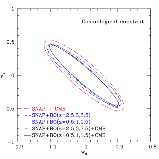
Figure 4: As Fig. 2, for baryon oscillation measurements and a cosmological constant model. The baryon oscillation data is slightly stronger than the CMB data but not very complementary with it.

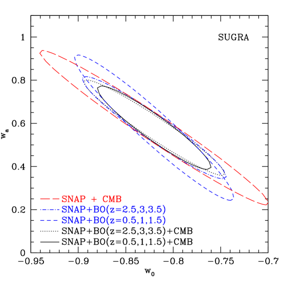
Figure 5: As Fig. 4 but for a supergravity inspired dark energy model. Now baryon oscillation and CMB data are more complementary with each other as well as the supernova data, so the improvement with all three is more pronounced.

Because of the insensitivity of the baryon oscillation results to the exact redshift range, so long as $z\mathrel{\mathchoice{\lower 3.6pt\vbox{\halign{$\mathsurround=0pt\displaystyle\hfil#\hfil$\cr>\crcr\sim\crcr}}}{\lower 3.6pt\vbox{\halign{$\mathsurround=0pt\textstyle\hfil#\hfil$\cr>\crcr\sim\crcr}}}{\lower 3.6pt\vbox{\halign{$\mathsurround=0pt\scriptstyle\hfil#\hfil$\cr>\crcr\sim\crcr}}}{\lower 3.6pt\vbox{\halign{$\mathsurround=0pt\scriptscriptstyle\hfil#\hfil$\cr>\crcr\sim\crcr}}}}1$, one can choose the survey characteristics based on observational considerations. As mentioned, at redshifts $z<1.5$ one is likely to detect only 1 or 2 baryon wiggles, making it more difficult to precisely determine the oscillation scale $k_{obs}$. But for $z>1.5$ the linear regime quickly extends in $k$-space, due to behavior of structure formation in a universe recently dominated by dark energy (see Fig. 1 of [12]), providing 3-4 detectable oscillations. The redshift ranges most advantageous for observations are often identified as $z=0.5-1.3$ and $z=2.5-3.5$ [14] due to easy selection by 4000Å break and Ly$\alpha$ features in the galaxies used in the survey. Estimates of number of galaxies required and sky coverage are given in [13, 14].

Such a redshift survey could be accomplished by large telescopes on the ground within a decade. One possibility is the KAOS project [18]: the Kilo-Aperture Optical Spectrograph proposed as a front end for the Gemini South 8 meter telescope. This would have multiplexing capability from some 4000 fibers for simultaneous measurement of galaxy redshifts. With a 1.5 square degree field of view and coverage of some 400 square degrees of sky KAOS could measure precise redshifts for $10^{6}$ galaxies. This could provide estimates of the wiggle scale at the 2% precision level [13].

Another intriguing idea is to use wide field observations from space. This would have the advantage of not being restricted to the $z\approx 1$ and 3 ranges just mentioned, which were limited by the Earth’s atmosphere. Indeed, from a theoretical point of view, a redshift range $z=1.5-2$ is essentially as powerful as $z\approx 3$ in terms of number of oscillations mapped, a definite advantage over $z\approx 1$, and yet requires less spectroscopic exposure time than the deeper survey. Calculations show that the parameter estimation for a given precision is as tight as the lower or higher redshift ranges.

While there is no planned massively multiplexing spectrograph for space, one interesting possibility is populating spare regions of the SNAP focal plane with grisms capable of low resolution spectroscopy. Also, photometric redshifts can be generated with SNAP’s nine filters. There is no problem achieving the number or area statistics as the proposed SNAP wide field survey (mostly focused on weak gravitational lensing) will find $10^{8}$ galaxies over 300 square degrees. However with a 2 meter telescope and spectral resolutions of order 100 or less, this clearly is not capable of carrying out all the science that an 8 meter ground based telescope with high resolution spectrograph could. Still, while this would not provide the same precision mapping of the 3D matter power spectrum, it might give decent quality information on the 2D, projected spectrum, roughly corresponding to the transverse wavenumber modes in Eq. (3). Photometric or low resolution spectroscopic redshifts would additionally give a smeared representation of the radial dimension. Detailed analysis of the baryon oscillation method with SNAP is left for future work; here we simply investigate the parameter constraints from the transverse and radial modes separately.

One expects that the radial mode, $d\tilde{\eta}$, which involves a bare factor $H(z)$, should provide better limits, while the transverse mode, $\tilde{\eta}$, acts basically like a distance-redshift measurement though with the important degeneracy differences previously mentioned. Indeed the sensitivities plotted in Fig. 3 bear this out (though the degeneracy relations are not there apparent; also note that the radial mode has low sensitivity at redshifts that are well into the matter dominated epoch). For example, denoting the full baryon oscillation information as BO, the radial only as BO_∥, and the transverse only as BO_⟂, one finds that 2% precision gives $\sigma(\Omega_{m})=0.0057$, $\sigma(w_{0})=0.069$, $\sigma(w_{a})=0.30$ for SN+CMB+BO, (0.0073, 0.073, 0.31) for SN+CMB+BO_∥, and (0.0065, 0.075, 0.35) for SN+CMB+BO_⟂. (Though presumably the precision in a full 3D survey would be better than in a 2D plus low resolution radial survey.) In the last case there is essentially no improvement over the SN+CMB case without any oscillation information. Various cases are illustrated in Fig. 6.

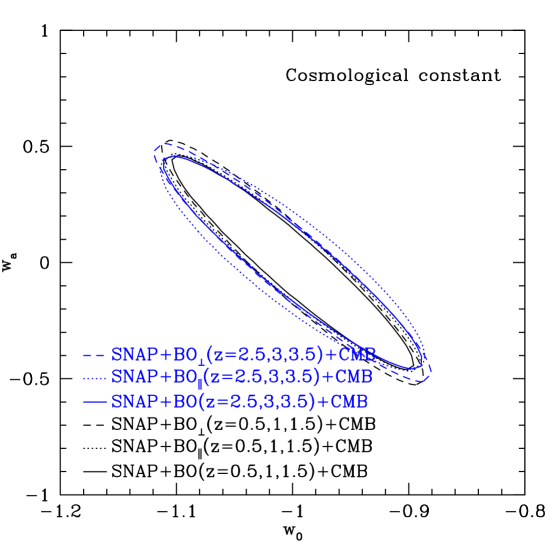
Figure 6: As Fig. 4 but separating the contributions from the baryon oscillation wave modes transverse and parallel to the line of sight. Radial information, requiring accurate redshifts from a spectroscopic survey such as KAOS, is more useful.

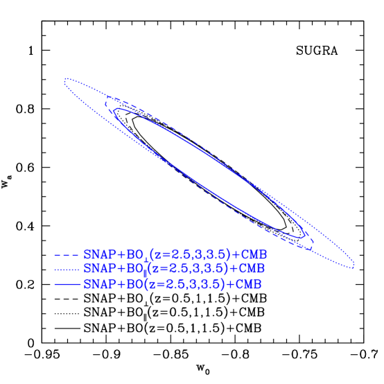
Figure 7: As Fig. 6 but for a supergravity inspired dark energy model. Now the transverse modes, detectable through a 2D survey, are more influential.

Again, the baryon oscillation method is more useful in the presence of a time varying equation of state dark energy. Moreover, due to the long baseline entering the integrated distance, the BO_⟂ information is actually more valuable than the radial, if at the same precision. The results for the SUGRA model are illustrated in Fig. 7. We see that 2% precision data on the transverse modes adds complementarity to the supernova and CMB information, improving the estimates of $\Omega_{m}$ by 56%, $w_{0}$ by 46%, and $w_{a}$ by 42%. This represents the vast majority of the impact of the full baryon oscillation data discussed at the beginning of this section.

5 Conclusion

Differential distance measurements, providing a snapshot of the expansion rate $H(z)$, have long seemed attractive theoretically as ways to probe the nature of dark energy. But they have also appeared difficult to implement observationally. The cosmic shear, or Alcock-Paczyǹski, probe (not to be confused with promising weak lensing shear measurements) involves a ratio of differential to integrated distances, or the product $H(z)\,r(z)$, and [5] showed that it could act only in a minor, complementary role to precision distance observations. The growth of structure in the linear regime also might be thought sensitive to $H(z)$ but at redshifts $z\mathrel{\mathchoice{\lower 3.6pt\vbox{\halign{$\mathsurround=0pt\displaystyle\hfil#\hfil$\cr>\crcr\sim\crcr}}}{\lower 3.6pt\vbox{\halign{$\mathsurround=0pt\textstyle\hfil#\hfil$\cr>\crcr\sim\crcr}}}{\lower 3.6pt\vbox{\halign{$\mathsurround=0pt\scriptstyle\hfil#\hfil$\cr>\crcr\sim\crcr}}}{\lower 3.6pt\vbox{\halign{$\mathsurround=0pt\scriptscriptstyle\hfil#\hfil$\cr>\crcr\sim\crcr}}}}2$ this essentially probes $\Omega_{m}$ not the dark energy; however, through other factors the linear growth still retains some sensitivity to the equation of state and its time variation [21]. Nonlinear structure formation can involve $H(z)$ as a separate factor through the differential volume element in cluster or galaxy halo counts, but this is entangled in systematic uncertainties from nonlinear physics and observational selection effects [19, 20]. On large scales this may be ameliorated, but the needed numerical simulations of large scale structure incorporating a time varying equation of state are just now being carried out [21].

In this paper we have pushed these observational difficulties into the background and considered the use of $H(z)$ regardless. Our conclusion is that it is not a panacea and only offers aid through complementarity with a deep, precision distance survey such as SNAP; then it contributes mild improvement to the cosmological parameter constraints. This is basically due to $H(z)$ acting at higher redshifts as a determinant of the matter density, not a direct probe of dark energy properties. At redshifts $z<1$ it has somewhat more leverage, but requires precision on the 1% level for significant improvement.

The baryon oscillation method of using wiggles in the matter power spectrum as a standard ruler determines a slightly different measure of the expansion rate $H(z)$. This probe is sufficiently promising, though again only in complementarity with a supernova distance survey, that it should be pursued further. Depending on the nature of the dark energy, incorporation of oscillation measurements can offer significant improvements on estimation of the time variation of the equation of state. One of the most striking aspects is its cleanness, based on simple, well understood physics and with no apparent major systematic uncertainties. Note that in all the analyses presented here of different cosmological probes, only the SNAP data has included systematic uncertainties – the $H(z)$ and baryon oscillation precisions have been taken as purely statistical. For all known and other proposed probes this is certainly overly optimistic. Whether systematics enter at the 1-2% level in the baryon oscillation method, from, say, residual nonlinearities or mass vs. light bias, needs further investigation.

Two interesting concepts for baryon oscillation observations are the KAOS project on the ground, and a spectroscopically less precise but reasonably straightforward space implementation with grisms or photometric redshifts from SNAP. We have seen that the optimal redshift range is not strongly determined by the parameter sensitivity, and so will be driven by trade offs in observation strategy. Both projects deserve further investigation, though it is intriguing to imagine that SNAP could represent a cosmology superprobe – incorporating the supernova distance, weak lensing, some part of the baryon oscillation, and possibly even cluster count methods of cosmological parameter determination. But even if SNAP is rather promising for revealing the nature of dark energy, our understanding and confidence will still be strengthened by multiple, complementary and crosschecking next generation surveys.

References

- [1] S. Perlmutter et al., Astrophys. J. 517, 565 (1999)
- [2] A. Riess et al., Astron. J. 116, 1009 (1998)
- [3] D.N. Spergel et al., astro-ph/0302209
- [4] W.J. Percival et al., MNRAS 337, 1068 (2002); astro-ph/0206256
- [5] E.V. Linder, astro-ph/0212301.
- [6] M. Tegmark, D.J. Eisenstein, W. Hu, R. Kron, astro-ph/9805117
- [7] E.V. Linder, Phys. Rev. Lett. 90, 091301 (2003); astro-ph/0208512
- [8] http://snap.lbl.gov ; G. Aldering et al., in SPIE Proceedings 4835; astro-ph/0209550
- [9] http://astro.estec.esa.nl/Planck
- [10] W. Hu and N. Sugiyama, Ap. J. 471 (1996) 542
- [11] D.J. Eisenstein and W. Hu, Ap. J. 496 (1998) 605; astro-ph/9709112
- [12] D. Eisenstein, in Proceedings from Wide-Field Multi-Object Spectroscopy; astro-ph/0301623
- [13] H. Seo and D. Eisenstein, in preparation
- [14] C. Blake and K. Glazebrook, astro-ph/0301632
- [15] R.R. Caldwell et al., astro-ph/0302505
- [16] E.V. Linder, astro-ph/9712159
- [17] P. Brax and J. Martin, Phys. Lett. B468, (1999) 40
- [18] http://www.noao.edu/kaos
- [19] J. Mohr, http://www.xray.mpe.mpg.de/~ringberg03/TALKS/Mohr.pdf
- [20] E.S. Levine, A.E. Schulz, and M. White, Ap. J. 577 (2002) 569; astro-ph/0204273
- [21] A. Jenkins and E.V. Linder, in preparation