Oxygen Gas Phase Abundance Revisited

Abstract

We present new measurements of the interstellar gas-phase oxygen abundance along the sight lines towards 19 early-type galactic stars at an average distance of 2.6 kpc. We derive O I column densities from HST/STIS observations of the weak 1355 Å  intersystem transition. We derive total hydrogen column densities [N(H I)+2N(H₂)] using HST/STIS observations of Lyman-$\alpha$  and FUSE observations of molecular hydrogen. The molecular hydrogen content of these sight lines ranges from f(H₂) = 2N(H₂)/[N(H I)+2N(H₂)] = 0.03 to 0.47. The average $\langle H_{tot}/E_{B-V}\rangle$ of 6.3$\times$10²¹ cm^-2 mag^-1 with a standard deviation of 15% is consistent with previous surveys. The mean oxygen abundance along these sight lines, which probe a wide range of galactic environments in the distant ISM, is 10⁶ (O/H)_gas = $408~{}\pm~{}13$ (1 $\sigma$ in the mean). We see no evidence for decreasing gas-phase oxygen abundance with increasing molecular hydrogen fraction and the relative constancy of (O/H)_gas suggests that the component of dust containing the oxygen is not readily destroyed. We estimate that, if 60% of the dust grains are resilient against destruction by shocks, the distant interstellar total oxygen abundance can be reconciliated with the solar value derived from the most recent measurements of 10⁶ (O/H)_gas⊙ = 517 $\pm$ 58 (1 $\sigma$). We note that the smaller oxygen abundances derived for the interstellar gas within 500 pc or from nearby B star surveys are consistent with a local elemental deficit.

1 Introduction

The chemical evolution of galaxies is a long-standing open question in astronomy (Audouze & Tinsley 1976). Of all atomic species, oxygen, which is mainly produced in type II supernovae, has proven to be the most useful element for probing the astration of the ISM by massive stars, both because of its large abundance and origin (for a review see Henry & Worthey 1999). The value of the oxygen abundance within a few hundred parsec from the Sun has been thoroughly investigated in the past two decades toward dozens of sight lines with Copernicus (De Boer et al. 1981, York et al. 1983, Keenan et al. 1985), HST (Meyer et al. 1998, Cartledge et al. 2001) and FUSE (Moos et al. 2002, and references therein). The accurate study by Meyer et al. (1998) revealed a well mixed medium within 500 pc from the Sun : $\langle{\rm O/H}\rangle=343\pm~{}15$ ppm (error in the mean). Note that this value has been corrected linearly with an updated f-value (see §3.3). However, investigations of more distant sight lines with the FUV absorption technique were limited by the unknown higher molecular fractions and the fainter background continua.

Measurements of oxygen abundances beyond 1 kpc have been carried out in two different environments : H II regions and B star atmospheres. To this day, these methods do not agree on a single picture for the oxygen distribution in the disk. In the most recent survey of the oxygen abundance in galactic H II regions, Deharveng et al. (2001) confirm the existence of a metalicity gradient from the center out to 18 kpc in the outer disk and find a local abundance consistent with ISM investigations. However they point out that their value is highly dependent on the model adopted for the electron temperature in the H II region. As for the B star surveys, the considerable scatter in the measurements makes it difficult to pin down an accurate value for the gradient (Smartt & Rolleston 1997, Primas et al. 2001) while, at the same time, the origin of the scatter is still debated.

With the high sensitivity of FUSE (10,000 times more sensitive than Copernicus; see Moos et al. 2000) it is now possible to probe the molecular hydrogen content of the ISM beyond 1 kpc and in denser media as well. Along with Lyman-$\alpha$ data from the STIS instrument, this allows us to obtain accurate total hydrogen column densities and hence derive a reliable O/H ratio. Since oxygen and hydrogen have about the same ionization potential, no ionization correction is needed and the analysis is largely model independent. The principal question we try to answer in this work is the robustness of a constant O/H for large sight line distances. The sight lines studied sample a vast diversity of environments. The enhanced depletion of oxygen in dust grains along the densest sight lines, the imprint of the galactic gradient along the most distant sight lines and inefficient mixing processes are expected to play significant roles in the final scatter.

In this paper, we present new O/H measurements toward 19 lines of sight (Table 1) obtained with data from FUSE and STIS. For each one of these sight lines we performed a complete analysis of the O I, H I, and H₂ content, using different techniques. The datasets and the reduction processing are described in §2. The analysis of O I, H I, and H₂ are presented in §3. In §4 the results are discussed in view of the most recent investigations. Discussions about the dust content and local oxygen deficit are given in §5 and conclusions are given in §6.

2 Observations

2.1 STIS observations

In this work, we use high-resolution STIS echelle observations of 19 stars (Table 1) to derive the column densities of H I, O I, and other atomic species. The design and construction of STIS are described by Woodgate et al. (1998), while information about the on-orbit performance of STIS is summarized by Kimble et al. (1998). A summary of the STIS observations is given in Table 2.

All observations in this work used the far-ultraviolet MAMA detector with the E140H grating. Because the datasets are drawn from several programs, three different apertures were used in obtaining the data. The $0\farcs 1\times 0\farcs 03$ aperture (the so-called “Jenkins slit”) provides a spectral resolution of $R\equiv\lambda/\Delta\lambda\approx 200,000$ (velocity resolution of $\Delta v\sim 1.5$ km s^-1, FWHM). These datasets have been discussed by Jenkins & Tripp (2001). The remainder of the data, taken through the $0\farcs 2\times 0\farcs 09$ or $0\farcs 2\times 0\farcs 2$ apertures, provide a spectral resolution of $R\approx 110,000$ (velocity resolution of $\Delta v\sim 2.7$ km s^-1, FWHM). Data taken through the latter apertures have a line spread function (LSF) with power in a halo extending $\sim\pm~{}5$ km s^-1 from line center. The LSF for all of the data have weak, broad wings stretching to $\pm~{}10$ km s^-1 (see the STIS Instrument Handbook).

The data were calibrated and extracted and the background estimated as described by Howk & Sembach (2000a). For spectral regions covered in multiple orders, or when more than one observation existed, we co-added the flux-calibrated data weighting each spectrum by the inverse square of its error.

2.2 FUSE observations

This work makes use of FUSE observations for deriving molecular hydrogen column densities along the 19 lines of sight studied. These column densities are in turn used to derive the total (atomic+molecular) hydrogen column densities along each sight line.

The FUSE mission, its planning and on-orbit performance are discussed by Moos et al. (2000) and Sahnow et al. (2000). Briefly, the FUSE observatory consists of four co-aligned prime-focus telescopes and Rowland-circle spectrographs that produce spectra over the wavelength range 905-1187 Å with a spectral resolution of $\sim$ 15-20 km s^-1 for point sources (depending on the wavelength). Two of the optical channels employ SiC coatings providing reflectivity in the wavelength range $\sim$ 905-1090 Å while the other two have LiF coatings for maximum sensitivity above 1000 Å. Dispersed light is focused onto two photon-counting microchannel plate detectors.

Table 3 presents a summary of the FUSE observations used in this work. All of the datasets were obtained through the large 30″$\times$30″ (LWRS) aperture. The two-dimensional FUSE spectral images were processed using the standard CALFUSE pipeline (version 1.8.7). The reduction and calibration procedure includes thermal drift correction, geometric distortion correction, heliocentric velocity correction, dead time correction, and wavelength and flux calibration. The observations of each star were broken into several sub-exposures, which were aligned by cross-correlating the individual spectra over a short wavelength range that contained prominent spectral features. The aligned sub-exposures were co-added, weighting each by the exposure time. No co-addition of data from different channels was performed; instead each channel was used independently in the fitting procedure as a different measurement.

3 Analysis

In this section we discuss the analysis of atomic species O I, H I, Kr I, and molecular hydrogen (H₂). Whenever possible we compare our results with those found in the literature. The analysis of H I (from STIS data) and H₂ (from FUSE data) are described respectively in sections §3.1 and §3.2. §3.3 discusses the analysis of O I with other atomic species (using STIS data).

3.1 H I Analysis

One of the most important factors limiting the accurate measurement of the O/H ratio is the uncertainty associated with the available H I measurements, which are derived primarily from analyses of the damping wings of H I Lyman-$\alpha$. For OB stars, the uncertainties in the H I measurements are largely systematic, particularly due to the complexity of the stellar continuum against which the interstellar Lyman-$\alpha$ is viewed. The systematic uncertainties can be minimized, however, in some cases by using high signal-to-noise datasets to probe further into the core of the Lyman-$\alpha$ profile (e.g., Howk et al. 1999a).

We have endeavored to measure the H I column densities towards the stars in our sample, making use of the STIS E140H spectra discussed above. Because the Lyman-$\alpha$ transition covers several Å, we have co-added several echelle orders for our analysis. The CALSTIS flux calibration of the E140H data shows a systematic error in that the short wavelength portion of an order $m$ shows a larger flux than the long wavelength portion of the order $m+1$. We have corrected this by applying a polynomial flux correction to each order. The correction was assumed to be the same for each order within an observation and derived from a comparison of STIS and GHRS data of HD218915. Unfortunately no other GHRS target was available for this comparison but we are confident in our correction for it produces a symmetrical profile of the Lyman-$\alpha$ transition in each spectrum. We used a weighted average scheme to combine adjacent flux-corrected orders.

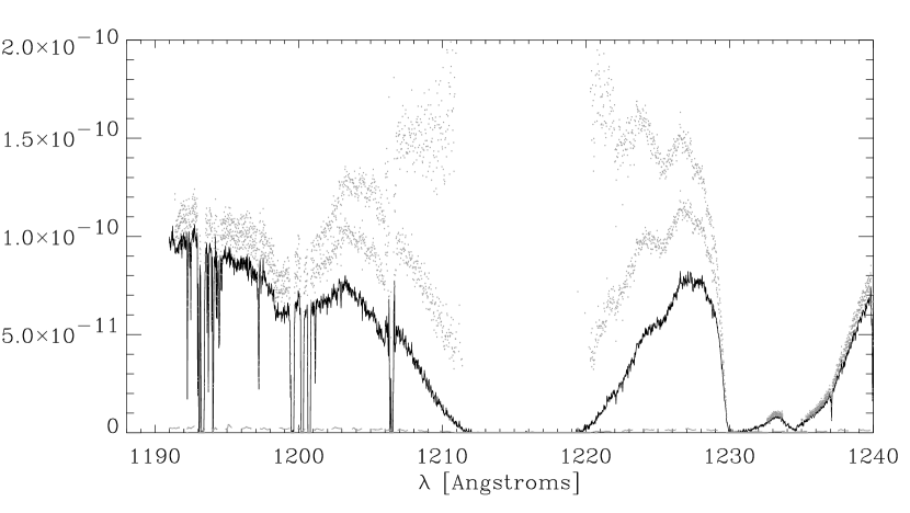
Figure 1: Example of Lyman-$\alpha$ continuum reconstruction for HD210839. The black continuous line represents the data, the gray points are the reconstructed continua. Each of these continua is at least two sigma above and below from the true continuum. Note the steep absorption feature on the red wing of Lyman-$\alpha$ associated with stellar wind.

Given the confusing presence of stellar photospheric and wind lines in the region near interstellar Lyman-$\alpha$, we make use of the continuum reconstruction method (Bohlin 1975; Diplas and Savage 1994; Howk et al. 1999a) for deriving N(H I). This method multiplies the observed Lyman-$\alpha$ profile by $\exp^{(+\tau_{\lambda})}$, where $\tau_{\lambda}$ is the optical depth as a function of wavelength. The H I column density is determined by the value of $\tau\,[\propto N(\mbox{H~{}{\small I}})]$ which best reconstructs the damping wings of Lyman-$\alpha$ to the estimated position of the stellar continuum. The method relies on human judgment to set the stellar continuum, which is not rigorously defined given the undulating stellar absorption features. For each of the stars, two authors have independently determined the $\pm$ 2 $\sigma$ limits following Howk et al. (1999a) with the final value being negotiated between them. The $\pm$ 2 $\sigma$ limits are those column densities which showed reconstructed continua that were highly implausible. The best fit values were then calculated to be the midpoint, assuming symmetric errors. Finally, we find that our column densities are, in all cases, within $1~{}\sigma$ of those given by Diplas & Savage (1994). However, the higher signal to noise ratio of our HST data allows us to use regions closer to the line core, leading to smaller systematic uncertainties. An example of this procedure is shown in Figure 1, where the reconstructed continua for HD210839 are displayed.

One potential difficulty in the H I analysis is the contamination of the ISM Lyman-$\alpha$ profile by stellar H I. In particular, for stars earlier than B2 the contamination is important for “low” interstellar column densities ($\log N(\mbox{H~{}{\small I}})\lesssim 20.5$; see Diplas and Savage 1994). Since our sight lines probe long pathlengths, most of which are in the galactic disk, we are always in the regime where $\log N(\mbox{H~{}{\small I}})>21$. Therefore, the corrections for stellar Lyman-$\alpha$ are always negligible.

We have tested the consistency of our Lyman-$\alpha$ H I analysis for nine of our targets using the higher-order Lyman transitions in the FUSE spectra of these stars. For the other stars, the blending of H₂ and H I is too severe to adequately check the N(H I) determination. For each of these nine targets, we constructed a complete model of the line of sight (velocity components, atomic and molecular content) which was then compared with the FUSE profiles of the weaker H I transitions. These models provided two checks of our Lyman-$\alpha$ analysis: first, they confirmed, using the weak damping wings of Lyman-$\beta$, the total H I column derived from the STIS data (although with larger uncertainties); second, modeling the high-order lines ruled out the existence of high velocity, low-$N(\mbox{H~{}{\small I}})$ components which might adversely affect our simple assumptions about the distribution of Lyman-$\alpha$ optical depth with wavelength (see Appendix A of Howk et al. 1999a). This eliminated a potentially significant bias in our H I column density determinations caused by hot, low column-density clouds similar to those discussed in this context by Lemoine et al. (2002) and Vidal-Madjar & Ferlet (2002) for sight lines through the local ISM.

3.2 H₂ Analysis

The FUSE bandpass contains some 20 ro-vibrational bands of molecular hydrogen (see, e.g., Shull et al. 2000; Tumlinson et al. 2002) which can be used for the determination of H₂ column densities. Most of the sight lines studied here lie predominantly within the galactic disk and have quite high molecular hydrogen column densities. We adopt wavelengths, oscillator strengths, and damping constants for the molecular hydrogen transitions from Abgrall et al. (1993a) for the Lyman system and Abgrall et al. (1993b) for the Werner system.

Our analysis of H₂ with the FUSE data makes use of the $Owens$ profile fitting software (Lemoine et al. 2002, Hébrard et al. 2002a) to fit the H₂ line profiles assuming a single Maxwellian component. We assume that the FUSE LSF is well described by a single Gaussian with a FWHM of 20 km s^-1. While this is an oversimplification of the FUSE LSF (see Wood et al. 2002, Hébrard et al. 2002a), it is sufficient for our purposes.

In the course of determining the H₂ content, we proceed in two steps. First, we analyse the population of the rotational levels J=2 and 3 that contain information on the excitation temperature within the gas. Although most of the corresponding absorption lines are deeply saturated, a few lines are weak enough to be near the linear part of the curve of growth, thereby allowing us to get reliable column density estimates. The profile fitting is done simultaneously over the different absorption lines ($\approx$ 10 spectral windows).

Then, we investigate the J=0 and 1 rotational levels that represent more than 90% of the total H₂ column density. For all of the sight lines presented in this work, the strongest J=0,1 lines show damping wings implying $N({\rm H}_{2})\gtrsim 10^{18}$ cm^-2 (Tumlinson et al. 2002). The specifics of the unresolved component structure were unimportant for these rotational levels. The main difficulty in analyzing these lines is determining the stellar continuum. Catanzaro et al. (2001) showed that, for early type stars with low rotational velocities, stellar continua are relatively smooth and featureless over the v1-0 and v2-0 ro-vibrational bands. We follow Catanzaro et al. (2001) in analyzing the J=0 and J=1 levels using the v1-0 and v2-0 Lyman bands. The J=0 transitions in these bands are centered at $\lambda\sim 1092$ and 1077 Å. The profile fitting is simultaneously performed over 5 spectral windows corresponding to the different channels. An example of the fit quality is shown in Figure 2.

We find that the rotational levels J=2 and 3 represent only a few percent of the total H₂ column density in all lines of sight studied here. As a result, they make relatively minor contributions to the error budget. Finally the errors are dominated by uncertainties in the continuum placement near the strong J=0,1 H₂ transitions. We have estimated the contribution of the continuum-placement uncertainties by fitting the data with three different continua: the best continuum, the best continuum plus 10%, and the best continuum minus 10%. We then assume that the H₂ column densities derived with the $\pm$ 10% continua represent $1~{}\sigma$ deviations from the best-fit columns.

Table 4 presents the derived H₂ column densities for each line of sight, as well as the fractional abundance of molecular hydrogen, $f({\rm H}_{2})\equiv 2N({\rm H}_{2})/[N({\rm H\ I})+2N({\rm H}_{2})]$ and the T₀₁ rotational temperature. We have compared our H₂ results with previous analyses of the FUSE data along two high extinction cloud sight lines studied by Rachford et al. (2002). In Table 5 we compare our results with theirs.

3.3 O I Analysis

To determine the column density of oxygen along our 19 sight lines, we use the weak O I intersystem transition at 1355.598 Å; the extreme weakness of this transition allows us to avoid most of the saturation effects seen in the other O I lines observable by STIS and FUSE. In agreement with Meyer (2001),we adopt the f-value for the 1355 Å transition suggested by Welty et al (1999): f=$1.16\times 10^{-6}$. This value was derived from the mean of the lifetime measurements of Johnson (1972), Wells and Zipf (1974), Nowak, Borst and Fricke (1978) and Mason (1990) and the theoretical branching fraction of Biémont and Zeippen (1992). This value is slightly smaller than the one previously adopted ($1.25\times 10^{-6}$, Morton 1991). When comparing our results with previous works that make use of the older f-value, we linearly correct their column densities to reflect our choice of oscillator strength. Our derived errors do not include uncertainties in the f-value (which are in large part unknown).

Although the O I 1355 Å line is typically quite weak, the presence of cold components with significant amounts of matter could cause difficulties when deriving the O I column densities if the lines are sufficiently narrow to be unresolved by STIS. We used 2 different approaches to derive the O I column densities: profile fitting (PF) and the apparent optical depth (AOD) method. The AOD method (Savage & Sembach 1991, Lehner et al. 2002) yields apparent column densities, N_a, that are equivalent to the true column density if no unresolved saturated structure is present. If such structure is present, then N${}_{a}~{}<$ N, and the apparent column density is a lower limit to the true column density. Our AOD analysis, including estimation of the errors, follows the procedures outlined in Sembach & Savage (1992).

Profile fitting, in which a detailed component model of the interstellar absorption is compared with the data, was performed with the profile fitting code $Owens$ developed by Martin Lemoine and the FUSE french team. We assume that the STIS LSF is well represented by a Gaussian with a FWHM of 2.67 km s^-1 for the spectra obtained through the $0\farcs 2\times 0\farcs 09$ and $0\farcs 2\times 0\farcs 2$ slits. For the $0\farcs 1\times 0\farcs 03$ slit the adopted LSF is a Gaussian with a FWHM of 1.5 km s^-1. The errors were calculated with the $\Delta\chi^{2}$ technique for each of the fitted components (Hébrard et al. 2002a, Lemoine et al. 2002). The profile fitting analysis of the O I column density was done simultaneously with other atomic species with absorption lines visible in the STIS data. Each fit made use of the following species to constrain the line of sight velocity structure: Cl I $\lambda$1347, C I $\lambda$1276 and C I $\lambda$1270, S I $\lambda$1295 and Kr I $\lambda$1235. Results of the fits for these species will be presented in a companion paper. Cl I and S I are useful tracers of dense clouds, while C I also traces cool material along diffuse lines of sight. Because these atomic species have different masses we were able to constrain the kinetic temperature and the non-thermal broadening for each component along the line of sight. An example of the full fit to all of the atomic species is shown in Figure 3 for the sight line towards HD210839. Figures 4 and 5 show the resulting fits for O I along the 19 sight lines.

Table 6 shows the comparison between the results obtained with the two methods, the equivalent width and the adopted N(O I). The adopted values are weighted averages of the two techniques, while the adopted uncertainties are the largest of the two errors. Previous O I measurements can be found in the literature for six of our targets: HD75305, HD104705, HD177989, HD185418, HD218915 and HD303308. Our measurements are compared with the literature values in Table 5. With one exception our results are consistent with previous measurements, within 1 $\sigma$. For the sight line towards HD218915, we found that there is no need for the saturation correction applied by Howk et al (2000), so our value is 30% smaller than previously stated.

Meyer et al. (1998) and Cartledge et al. (2001) have discussed the use of Kr I, a noble gas, as a proxy for neutral hydrogen, demonstrating the relative constancy of O/Kr in local gas. For four stars we were able to derive Kr I column densities, which, when compared with the O I column densities, offer another opportunity to compare our results with others. Table 7 summarizes our O/Kr measurements, showing that our measurements are consistent with previous results.

4 The oxygen abundance

4.1 The sample

The dataset is composed of 19 sight lines toward distant stars ranging from .8 to 5.0 kpc. The average distance from the Sun is 2.6 kpc while the average galactocentric radius is 7.7 kpc. We are thus probing material well beyond the local ISM. The average distance from the Sun in our sample is about 5 times the one found in Meyer et al (1998): $\langle$d$\rangle$ = 530 pc. The molecular fraction ranges from 3% to 47% while the E_B-V ranges from 0.16 to 0.64. Although most of our sight lines are “translucent sight lines” as defined in Rachford et al (2002), a handful are purely diffuse sight lines with the gas largely in the local ISM.

As shown in Table 1, the stars studied in this work are mostly distributed in the disk of the Galaxy with a few of them being in the low halo ($|z|$ $>$ 250 pc): HD88115, HD99857, HD157857, HD218915, and HD177989. HD177989 is the most distant star in the sample (5 kpc) and is, at the same time, the highest above the galactic plane with $|z|$=1032 pc. This line of sight goes through the ejecta of the Scutum supershell (GS 018-06+44), in the Scutum spiral arm. Previous observations carried out by Savage et al. (2001) reveal strong and broad absorption in the lines of Si IV and C IV centered on LSR velocities of +18 and +42 km s^-1 and weaker absorption from these ions near $-$50 and $-$13 km s^-1. However, the neutral gas does not show any signature of these weak high velocity components.

Among the densest sight lines in our dataset are HD210839 and HD192639 with E_B-V=0.62 and 0.64, respectively. HD210839 is much closer to the Sun than HD192639 and has been long recognized to have a peculiar extinction curve (Diplas & Savage 1994). The average density is about 80 hydrogen atoms per cubic centimeter as derived from O I excited lines (Jenkins & Tripp 2001). New diffuse interstellar band features (DIBs) have also been reported recently toward this star (Weselak 2001). With the highest molecular fraction of our sample (47%) this sight line is likely to probe dense material in which the oxygen might be more depleted onto grains. HD192639 is part of the Cyg OB1 association located at 1.8 kpc from the Sun. However, for this latter sight line a deep investigation of the C I transitions with the STIS E140H echelle, by Sonnentrucker et al. (2002) shows that there is a dense, albeit relatively small, knot along this sight line, which has diffuse global properties (with an expected average of 11 atoms cm^-3).

Two peculiar sight lines in our sample show intermediate velocity components: HD93205 and HD93222. Both of these stars are part of the Carina nebula and are only 400 parsec away from each other. In a recent survey of the Carina nebula (Garcia & Walborn 2000), it has been demonstrated that the high and intermediate velocity structures are produced by an interaction between the stellar winds of the earlier type stars and immediately surrounding interstellar material. Small angular variations in Na I and Ca II abundances are typical in this nebula and we shall expect the same for the oxygen abundance if the absorption is mainly due to the surrounding clouds.

4.2 Results

Table 6 summarizes all the measurements performed for (O/H)_gas. Using the 19 stars of the sample, we find a mean abundance of (O/H)_gas = 408 ppm with an error in the mean of 13 ppm. The error in the mean we report here is the weighted average variance which is computed with the individual error estimates and the scatter around the mean. We also computed the a priori estimate of the error in the mean using only the individual error estimates. While this usually should give a smaller value, we find 14 ppm and this result strongly suggests that some of our errors have been overestimated. The weighted average variance is certainly a more reliable estimate for the error in the mean in this case. Throughout this section, we also use the weighted average variance as the best estimate of the error in the mean when comparing different samples. The straight standard deviation is 59 ppm and represents only a 15% deviation from the mean. The reduced $\chi^{2}$ of 0.9 indicates that the scatter is consistent with the errors assuming a Gaussian parent distribution around a constant value.

If we only consider the low halo targets ($|z|>250$ pc), we have 5 stars with a mean of (O/H)_gas = $394\pm~{}24$ ppm. These sight lines to halo stars appear to be statistically consistent with the rest of the sample; this is due to the fact that these sight lines are probing mostly disk material. In particular, in the case of HD177989, we have seen that none of the typical velocity structures associated with high-z features along this sight line are detected in the neutral gas.

The fact that we find a homogeneous oxygen abundance throughout the disk contrasts with the large scatter reported in stellar atmospheres studies (Smartt & Rolleston 1997, Primas et al. 2001). It could be that this scatter vanishes as we integrate the column density over long pathlengths. On the other hand, our scatter is consistent with the rms scatter found in the H II survey by Deharveng et al. (2000) ($\approx$ 22 %) and is also consistent with the picture of an efficient mixing of oxygen in the galactic disk as shown by theoretical calculations (see Roy & Kunth 1995).

The constancy of the oxygen abundance holds for a large range of molecular fractions as shown in Figure 6. It is remarkable to observe that, although many of the targets in our sample have molecular fractions similar to the ones reported in Cartledge et al. (2001), we do not report any trend toward an enhanced oxygen depletion. One possible explanation is that the sight lines in our sample are made of a mixture of diffuse and dense clouds and are indeed dominated by the diffuse components in most cases, contrary to the most reddened sight lines in their study which are spatially associated with dark cloud complexes. However, in the case of the sight line toward HD210839, which presents both high E_B-V and large density (80 hydrogen atoms per cubic centimer), we still do not detect the hint of an enhanced oxygen depletion reported by Cartledge et al. (2001).

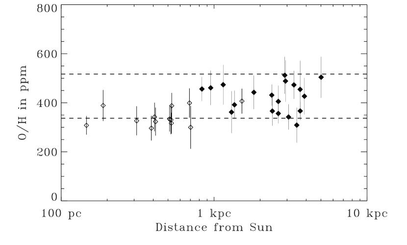
Figure 7: O/H versus distance from the Sun. Filled diamonds are our new measurements in the distant ISM, open diamonds are local measurements from Meyer et al. (1998). The upper dashed line represents the total oxygen abundance (solar value) and the lower dashed line represents what is left when the maximum amount of oxygen (180 ppm) is depleted into grains. All the measurements are expected to lie within these two limits. However, we note that, for pathlengths smaller than 1 kpc, points cluster around the lower limit and a little below.

In order to test how much the oxygen abundance is varying with distance and density we combine our measurements with measurements from the recent literature. The 13 sight lines from Meyer et al. (1998) are similar to the sight lines in our sample (referred as sample A) in the sense that they are mostly diffuse and are not expected to show O I enhanced depletion onto grains. Noteworthy, the average distance in sample A is about one order of magnitude larger than in the Meyer et al. (1998) sample. The comparison of the mean (O/H)_gas also reveals a systematic 16% underabundance of oxygen within 500 pc, as illustrated in Figure 7.

By combining Meyer et al. (1998) values with ours, we get a sample of 32 sight lines (sample B) in which the distances range from 150 pc to 5 kpc. We find a mean (O/H)_gas of 377 ppm with an error in the mean of 10 ppm. Finally, we include 5 measurements performed through denser media by Cartledge et al. (2001): HD27778, HD 37021, HD37061, HD147888 and HD207198. While the distances of these 5 stars are comparable to the distances found in sample A, the sight lines are different in nature being probably a lot denser. This final sample (sample C) is made of 37 sight lines with a wide variety of properties: the total hydrogen column density ranges from 1.5$\times$10²⁰ cm^-2 to 62$\times$10²⁰ cm^-2, log f(H₂) from -5.21 to -0.2, the reddening from 0.09 to 0.64 and the distance to the Sun from 150 pc to 5 kpc. Table 8 summarizes the oxygen abundance found in the different samples. In particular, we see that in sample C, although the scatter is the largest, the standard deviation is only of the order of 20% around the mean of 362 ppm.

From the 19 measurements of the total hydrogen in sample A, we derive an average $\langle$ H_tot/E_B-V $\rangle$ of 6.3$\times$10²¹ cm^-2 mag^-1 with a standard deviation of 9$\times$10²⁰ cm^-2 mag^-1 (Figure 8). This value is fully consistent with the known galactic averages $\langle$ H₂/E_B-V $\rangle$ = 5$\times$10²⁰ cm^-2 mag^-1 (Dufour et al. 1982), $\langle$ H I/E_B-V $\rangle$ = 4.93$\times$10²¹ cm^-2 mag^-1 (Diplas & Savage 1994) implying $\langle$ H_tot/E_B-V $\rangle$ = $\langle$ H I/E_B-V $\rangle$ + 2 $\langle$ H₂/E_B-V $\rangle$ = 5.93$\times$10²¹ cm^-2 mag^-1. The standard deviation we derive for this ratio is relatively small and is an indication that the total hydrogen content and the dust are well correlated in our sample. Finally, we point out that oxygen column density and reddening seem to be comparable tracers of the total hydrogen column density over a wide range of distances and densities.

5 Discussion

5.1 Dust grains

The role of oxygen is fundamental in modern dust models. It is known to be abundant in the cores of silicate dust grains (Hong & Greenberg 1980). In particular, the maximum amount of oxygen atoms tied up into grains is limited by the abundance of metals with which oxygen bonds (O:Si:Mg:Fe) $\approx$ (24:1:1:1). A theoretical upper limit to the number of oxygen atoms that can be incorporated into grains is then calculated assuming that all grains are made of silicates (Cardelli et al. 1996): (O/H)_dust $\leq 180$ ppm. It was long believed that this value was too small to reconciliate the gas phase ISM oxygen abundance with the solar value. However, recent measurements of the solar oxygen abundance by Holweger (2001) and Allende et al. (2001) have revised the solar abundance downward significantly. Allende et al. (2001) derived a mean solar oxygen abundance of 490 $\pm$ 59 ppm while Holweger (2001) derived a similar value (although with larger errors) with $({\rm O/H})_{\odot}$= 545 ppm $\pm$ 100 ppm. In the following we adopt a straight average of their values as the solar abundance : $({\rm O/H})_{\odot}=517\pm~{}58$ ppm. This value is now in good agreement with the maximum total abundance (gas+dust) derived using our gas-phase O/H measurements combined: (O/H)_gas + (O/H)${}_{\rm{dust}}~{}\lesssim 408\ {\rm ppm}\,+\,180\ {\rm ppm}\,\lesssim 588\,{\rm ppm}$. Thus it would seem that the total interstellar oxygen abundance is now consistent with the best solar oxygen abundance.

If we assume that the solar value reflects the total oxygen abundance in the ISM and that the total oxygen abundance is constant, we can then estimate the average dust oxygen content for our sight lines. We find $\langle$(O/H)${}_{\rm{dust}}\rangle$ = 109 ppm with a standard deviation of about 60 ppm. Since we know the maximum amount of oxygen atoms that can be tied up into silicate grains (O/H)_dust = 180 ppm), then, from our survey, we find that $\approx$ 60% of the grains are resilient against destruction by shocks on average, with one extreme sight line showing nearly 100% destruction and others showing no destruction at all. Along the sight line toward HD93222, which probes material surrounding the star (see §4.1), most of the oxygen atoms have been released in the gas phase. This can be interpreted as the effect of the interaction between the stellar wind and the nearby ISM. On the other hand, the three most oxygen depleted sight lines in sample C are from the Cartledge et al. (2001) survey in the dense ISM, consistent with an enhanced depletion into dust grains. Finally, this is also consistent with the theoretical expectation that only 10 to 15% of the grains are destroyed at each passage of a 100 km s^-1 shock in the warm ISM (Tielens et al. 1994, McKee et al. 1987). Such shocks are believed to be responsible for most of the grain destruction and could explain the observed population of resilient dust grains. These shocks could also explain the variations in oxygen bearing dust. Several other indirect pieces of observational evidence support the view that dust grains are long-lived, among them the abundance studies toward the diffuse halo clouds by Sembach & Savage (1996) and the detection of dusty structures in the halo of spiral galaxies by Howk & Savage (1999b). Both observations imply that a fraction of the grains can survive for a long time before being destroyed by thermal sputtering in the halo.

5.2 Local oxygen deficit

Meyer et al (1998) showed that the local oxygen abundance is remarkably constant. Our data, probing a wider range of environments at larger distances, show much the same. However, there is a systematic difference of 16% between the two samples that needs to be discussed in the context of a possible enhanced depletion within a few hundred parsecs from the Sun.

Previous studies of the local ISM have found some evidences for a global elemental deficit. Krypton abundance has been measured toward 10 stars in the local ISM by Cardelli et al. (1997) and a depletion of 1/3 was found when compared to the solar abundance. Because it is a noble gas, krypton is not expected to be depleted into the dust phase and this observation alone is a strong argument against the Sun being an appropriate cosmic standard for the nearby ISM. The same has been observed with sulfur, which is not supposed to be depleted in dust grains. The sulfur abundance derived from nearby B stars is about 2/3 of the observed ISM abundances beyond 2 kpc (Fitzpatrick & Spitzer 1993, 1995, 1997 and Harris & Mas 1986) and 2/3 of the solar sulfur abundance. The same depletion pattern is seen for oxygen when the solar value is compared to the nearby B stars while the comparison with distant B stars does not shed much light on the subject because of the large scatter (Smartt & Rolleston 1997). More generally, abundances have been measured in nearby B stars and young F and G field stars (see the summary by Snow & Witt 1996) and are consistently below solar for all measured elements. These star samples are representative of the current local ISM and clearly point toward a local elemental deficit.

Meyer et al. (1998) have reviewed the possible scenarios to explain such a depletion pattern: presolar nebula enrichment, radial migration of the Sun and infall of metal-poor gas. The oxygen abundance we derive from outside the local ISM can be used as a test for the latter scenario. As far as the oxygen abundance is concerned, the presolar nebula enrichment and the Sun migration might be discarded because of the apparent consistency between the solar value and the total oxygen abundance of the distant ISM. The recent infall of metal-poor material seems to be consistent with our present observation that the oxygen gas-phase abundance is slightly higher beyond 1 kpc. This is expected to be the case if the Gould belt has been created by an infalling cloud (Comeron & Torra 1994). Infall is considered as an important component of galactic chemical evolution and is supported by evidence for the infall of low-metalicity clouds onto the Milky Way (Richter et al. 2001). In this scenario the dilution should have affected all the elements the same way and the local oxygen enhanced depletion is expected to be the same as observed in krypton and sulfur: about one third.

However, the difference between our value, (O/H)_gas = $408$ $\pm$ 13 ppm beyond 1 kpc and the value found by Meyer et al. (1998), (O/H)_gas = $343$ $\pm$ 15 ppm within 1 kpc, is only one sixth. A possible explanation for a reduced dilution of oxygen in the local ISM is the destruction of a fraction of the dust grains that resulted from the impact of a low metalicity cloud, at an estimated velocity of 100 km s^-1 (Comeron & Torra 1994). However, in this scenario, we should expect that many metals were released in the gas-phase as well. It is beyond the scope of this paper to explore the different infall scenarios that might be consistent with the observations.

5.3 The galactic gradient

Some of the stars in our sample are sufficiently distant that the measurements might be affected by large scale abundance gradients in the ISM. Of course the gradient is in part masked by the integrated nature of our absorption lines and by the intrinsic scatter between sight lines. An extreme example of intrinsic scatter between the data points is given by the couple HD93222/HD93205. Both are members of the Carina nebula (Garcia & Walborn 2000) and show intermediate velocity structures in their spectra due to stellar winds interacting with surrounding material. It is well known that in this nebula the spatial variation of Na I as well as Ca II can be as large as 50%. Although they are within 400 pc of each other, the oxygen abundances we derive differ by as much as 43%. However the typical scatter between our data points is only of the order of 15% and this must be compared to the gradient effect expected in our data.

Numerous papers have discussed the distribution of heavy elements in spiral galaxies (see the review by Henry & Worthey 1999 and references therein). The published values by Deharveng et al. (2000), using H II regions, and by Smartt & Rolleston (1997), using B stars, give the range of expected values for the oxygen gradient $\alpha$: -0.07$\pm~{}0.01$ dex kpc^-1 $<~{}\alpha~{}<$ -0.039$\pm~{}0.005$ dex kpc^-1. It is difficult, if not impossible, to use the velocity of the absorbers to deduce a precise location within the disk assuming the most recent galactic rotation curve. The reason is that, except in a few cases, the expected velocities in the local standard of rest along our sight lines are within the typical scatter (around 7 km$s^{-1}$). Thus, we choose to show the oxygen abundance as a function of the location of the background star, expecting the gradient to show up as well. Figure 9 allows the comparison of the extreme $\alpha$ values with our data (excluding the peculiar sight lines HD93222 and HD93205). It turns out that the scatter of the points is largely dominated by the measurement errors while no large scale trend emerges at all.

6 Summary

In this paper we have presented a survey of the oxygen gas-phase abundance using STIS/FUSE data toward 19 stars with the purpose of probing the oxygen abundance far away in the disk. This work follows from previous surveys in the local ISM and is possible due to the FUSE detector’s sensitivity, which permits measurements of the H₂ content through long pathlengths. A summary of our results is as follow:

1. We demonstrate that the oxygen abundance shows little variation in various environments and various locations in the disk. We find a mean ratio of (O/H)_gas = 408 ppm with an error in the mean of 13 ppm. This is 19% higher than the mean previously derived in the local ISM by Meyer et al. (1998). We argue that a recent local infall of metal-poor material is not excluded as an explanation for the difference.

2. The oxygen abundance derived from our sample combined with previous surveys (37 sight lines) is consistent with both the oxygen abundance of young G & F stars ($\langle{\rm O/H}\rangle=456\pm~{}156$ ppm; Sofia & Meyer 2001) or the newly revised solar value ($\langle{\rm O/H}\rangle=517\pm~{}58$ ppm; Holweger 2001, Allende et al. 2001) once dust is taken into account.

3. Dust grains in the ISM are probably made of grain cores and we estimate that at least 60% of the grains have to be resilient in order to explain the difference between ISM and stellar abundances.

It is likely that the O I column density can be used as a surrogate tracer of the total neutral hydrogen column density, at least in a statistical sense, in diffuse ISM abundance studies. Although above we have emphasized the 19% difference between the mean (O/H)_gas found in this study and the lower value found for the LISM by Meyer et al. (1998), the most striking result from both studies is the lack of large deviations from the mean. The standard deviation in the sample reported here is 15%. If the Meyer et al. (1998) and the Cartledge et al. (2001) data are included, the standard deviation increases to only 20% for a wide variety of diffuse ISM conditions. The use of O I as a tracer of the total hydrogen column density could be of use in a variety of chemical abundance studies. As an example, consider the D/H studies, presently under way with the FUSE satellite. In many cases, determining accurate H I column measurements requires using HST or EUVE data, which may not be available. In other cases, because the column densities of D I and H I differ by about five orders of magnitude, accurate measurements of both species may be precluded by special conditions associated with a particular sight line. Preliminary studies of D/O ratios using FUSE measurements of D I and O I are encouraging (Moos et al. 2002, and references therein, Hébrard et al. 2002b). Additional studies are also needed to determine the special cases in which there are large deviations in the (O/H)_gas and identify the special conditions under which such deviations might exist (e.g Hoopes et al. 2003).

Figure 2: Fits of the low rotational levels (J=0, 1, 2) in the v2-0 (right) and v1-0 (left) bands for HD210839. For each of the spectral windows we used all the available FUSE segments (see Moos et al. 2000): LiF1A, SiC1A and SiC2B for v2-0; LiF2A and SiC2B for v1-0. Higher rotational transitions are indicated by the asterisks, they have been excluded from the fit.

Figure 3: This plot shows the fits of the atomic species for HD210839. This line of sight is an example of complex velocity structure with four components. Note that the signal to noise is low around the Kr I line due to the stellar wind absorption feature around 1235 Å.

Figure 4: Profile fitting of the O I $\lambda$1355 line. The numbers with ticks above the plot represent the velocity of each component. For each of these fits, we performed simultaneous profile fitting of C I $\lambda$1276, C I $\lambda$1279, Kr I $\lambda$1235, Cl I $\lambda$1246 and S I $\lambda$1295. Thus the information about the velocity structure and the b-values are well constrained. In the case of HD88115, the weak blue component is also detected by Jenkins & Tripp (2001).

Figure 5: Same comments as Figure 4. Note the noisy spectrum of HD210809 and the two weak O I components (detected in Cl I, C I and S I) dominated by the noise. This produces large errors for this line of sight.

Figure 6: The dashed line is the mean of the Meyer et al. (1998) sample: $({\rm O/H})_{gas}$=343 ppm. The long dashed line is the mean of our 19 sight lines: $({\rm O/H})_{gas}$=408 ppm. The error bars are 1 $\sigma$. Filled diamonds are our new measurements, open diamonds are Meyer et al. (1998) and open triangles are the Cartledge et al. (2001) measurements for which the molecular fraction is known. No enhanced depletion is seen for up to 47% of hydrogen atoms in H₂ within our sample. However, stars used in Cartledge et al. (2001) are both closer to the Sun and with a higher H I column density. They cross denser media in average and appear to be consistently below the mean.

Figure 8: The left panel shows the correlation between H I and E_B-V. We find H I/E_B-V = 4.9$\times$10²¹ cm^-2 mag^-1 and a standard deviation of about 25%. The correlation is much better between H_tot and E_B-V with a ratio of 6.3$\times$10²¹ cm^-2 mag^-1 and a standard deviation of 15% (right panel). Dust and gas are strongly correlated in our sample of diffuse sight lines.

Figure 9: O/H versus galactocentric distances. The upper dashed line represents the expected gradient from B star surveys (Rolleston et al 1997). The lower dashed line is the expected gradient from the H II survey by Deharveng et al. (2000). The location of the absorbers could be anywhere between the given stellar galactic radius and 8.5 kpc. All our values (filled diamonds) and the values from Meyer et al. (1998) (open diamonds) are within the range of the expected gradients. We excluded from this plot the two sight lines toward the Carina nebula (see §4.1). No trend is detected as a function of the stellar location. The vertical axis indicates the Sun’s galactocentric radius.

Table 1: Stellar properties.

Name	d	z	l	b	$E_{B-V}$	Spectral type
	[pc]	[pc]
HD75309	2405	80	265.9	-1.9	0.27	BI IIp
HD88115	3654	350	285.3	-5.5	0.16	B1 Ib/II
HD91824	2930	5	285.7	+0.1	0.27	O6
HD93205	2630	32	287.6	-0.7	0.45	O3 V
HD93222	2900	50	287.7	-1.0	0.36	O7 III
HD94493	3328	70	289.0	-1.2	0.20	B0.5 Iab/Ib
HD99857	3070	267	294.8	-5.0	0.33	B1 Ib
HD104705	3900	20	297.4	-0.3	0.26	B0 III/IV
HD124314	1150	8	312.7	-0.4	0.53	O7
HD157857	2380	548	13.0	+13.3	0.49	O7
HD177989	5010	1042	17.8	-12.0	0.25	B2 II
HD185418	950	33	53.6	-2.0	0.43	B0.5 V
HD192639	1830	48	74.9	+1.5	0.64	O7
HD202347	1300	45	88.2	-2.0	0.17	B1 V
HD210809	3470	188	99.8	-3.1	0.33	O9 Ib
HD210839	840	38	103.8	+2.6	0.62	O6 Iab
HD218915	3660	436	108.1	-6.9	0.29	O9.5 Iab
HD224151	1360	110	115.4	-4.6	0.44	B0.5 III
HD303308	2630	27	287.6	-0.6	0.45	O3 V

Table 2: Summary of HST observations.

Name	Dataset	Date	Exp. time (sec)	Aperture
HD75309	O5C05B010	03-28-99	720	$0\farcs 2\times 0\farcs 2$
HD88115	O54305010	04-19-99	1300	$0\farcs 1\times 0\farcs 03$
HD91824	O5C095010	03-23-99	360	$0\farcs 2\times 0\farcs 2$
HD93205	O4QX01010	04-20-99	1200	$0\farcs 2\times 0\farcs 09$
	O4QX01020	04-20-99	780	$0\farcs 2\times 0\farcs 09$
HD93222	O4QX02010	12-28-98	1680	$0\farcs 2\times 0\farcs 09$
	O4QX02020	12-28-98	1140	$0\farcs 2\times 0\farcs 09$
HD94493	O54306010	04-22-99	1466	$0\farcs 1\times 0\farcs 03$
HD99857	O54301010	02-21-99	1307	$0\farcs 1\times 0\farcs 03$
HD104705	O57R01010	12-24-98	2400	$0\farcs 2\times 0\farcs 09$
HD124314	O54307010	04-11-99	1466	$0\farcs 1\times 0\farcs 03$
HD157857	O5C04D010	06-03-99	720	$0\farcs 2\times 0\farcs 2$
HD177989	O57R03020	05-28-99	2897	$0\farcs 2\times 0\farcs 09$
HD185418	O5C01Q010	11-12-98	720	$0\farcs 2\times 0\farcs 2$
HD192639	O5C08T010	03-01-99	1440	$0\farcs 2\times 0\farcs 2$
HD202347	O5G301010	10-09-99	830	$0\farcs 1\times 0\farcs 03$
HD210809	O5C01V010	10-30-98	720	$0\farcs 2\times 0\farcs 2$
HD210839	O54304010	04-21-99	1506	$0\farcs 1\times 0\farcs 03$
HD218915	057R05010	12-23-98	2018	$0\farcs 2\times 0\farcs 09$
HD224151	O54308010	02-18-99	1496	$0\farcs 1\times 0\farcs 03$
HDE303308	O4QXO4010	03-19-98	2220	$0\farcs 2\times 0\farcs 09$
	O4QXO4020	03-19-98	1560	$0\farcs 2\times 0\farcs 09$

Note. — Distances, reddening and spectral types are from Diplas and Savage (1994) unless otherwise noted. The typical uncertainty in the distance is 30%.

Table 3: Summary of FUSE observations.

Name	Program ID	Date	Aperture	Exp. time (Ksec)	# exp.	Mode
HD75309	P1022701	01-26-00	LWRS	4.7	8	HIST
HD88115	P1012301	04-04-00	LWRS	4.5	8	HIST
HD91824	A1180802	06-02-00	LWRS	4.6	6	HIST
HD93205	P1023601	02-01-00	LWRS	4.7	7	HIST
HD93222	P1023701	02-03-00	LWRS	3.9	4	HIST
HD94493	P1024101	03-26-00	LWRS	4.4	7	HIST
HD99857	P1024501	02-05-00	LWRS	4.3	7	HIST
HD104705	P1025701	02-05-00	LWRS	4.5	6	HIST
HD124314	P1026201	03-22-00	LWRS	4.4	6	HIST
HD157857	P1027501	09-02-00	LWRS	4.0	8	HIST
HD177989	P1017101	08-28-00	LWRS	10.3	20	HIST
HD185418	P1162301	08-10-00	LWRS	4.4	3	TTAG
HD192639	P1162401	06-12-00	LWRS	4.8	2	TTAG
HD202347	P1028901	06-20-00	LWRS	0.1	1	HIST
HD210809	P1223101	08-05-00	LWRS	5.5	10	HIST
HD210839	P1163101	07-22-00	LWRS	6.1	10	HIST
HD218915	P1018801	07-23-00	LWRS	5.4	10	HIST
HD224151	P1224101	08-11-00	LWRS	6.0	12	HIST
HD303308	P1222601	05-25-00	LWRS	6.1	9	HIST
	P1222602	05-27-00	LWRS	7.7	12	HIST

Table 4: STIS and FUSE measurements of hydrogen

name	N(H I)	N(H2)	N(Htotal)	f(H2)	T01
	$10^{20}$ $cm^{-2}$	$10^{20}$ $cm^{-2}$	$10^{20}$ $cm^{-2}$		(K)
HD75309	11.2 (2.0)	1.5 (0.2)	14.2 (2.0)	0.21	65
HD88115	10.0 (2.0)	0.2 (0.1)	10.3 (2.0)	0.03	145
HD91824	11.7 (1.7)	0.7 (0.2)	13.1 (1.7)	0.11	65
HD93205	24.0 (2.3)	0.6 (0.1)	25.3 (2.3)	0.05	75
HD93222	25.1 (3.7)	0.6 (0.1)	26.4 (3.7)	0.05	121
HD94493	12.0 (1.2)	1.4 (0.2)	14.8 (1.3)	0.19	53
HD99857	17.4 (3.0)	2.7 (0.4)	22.8 (3.1)	0.24	53
HD104705	12.6 (2.5)	1.2 (0.1)	15.0 (2.6)	0.16	137
HD124314	25.7 (5.2)	3.3 (0.4)	32.3 (5.3)	0.20	54
HD157857	18.6 (2.3)	4.5 (0.6)	27.6 (2.6)	0.33	49
HD177989	9.1 (1.8)	1.5 (0.2)	12.1 (1.8)	0.25	88
HD185418	14.1 (2.5)	5.1 (1.3)	24.3 (3.6)	0.42	101
HD192639	19.5 (3.4)	5.5 (1.5)	30.5 (4.5)	0.36	98
HD202347	8.7 (1.8)	0.9 (0.2)	10.5 (1.8)	0.17	116
HD210809	17.8 (4.1)	1.3 (0.3)	20.4 (4.1)	0.13	166
HD210839	15.5 (1.9)	6.5 (1.0)	28.5 (2.8)	0.46	92
HD218915	14.8 (1.4)	1.6 (0.2)	18.0 (1.5)	0.18	56
HD224151	20.9 (3.6)	4.1 (0.6)	29.1 (3.8)	0.28	42
HD303308	25.7 (4.5)	2.2 (0.4)	30.1 (4.6)	0.15	54

Table 5: Comparison of our measurements with previous measurements.

Species	Stars	log N	log N	Reference
		this work	literature
O I	HD104705	17.81${}^{+0.02}_{-0.03}$	17.83$\pm~{}0.03$	Howk et al. 2000b
“	HD177989	17.79${}^{+0.02}_{-0.03}$	17.84$\pm~{}0.03$	“
“	HD218915	17.82${}^{+0.03}_{-0.03}$	17.97$\pm~{}0.03$	“
“	HD303308	18.09${}^{+0.02}_{-0.03}$	18.10$\pm~{}0.04$	“
“	HD192639	18.13${}^{+0.03}_{-0.02}$	18.16${}^{+0.11}_{-0.11}$	Sonnentrucker et al. 2002
“	HD75309	17.72${}^{+0.03}_{-0.04}$	17.73${}^{+0.05}_{-0.06}$	Cartledge et al. 2001
“	HD185418	18.05${}^{+0.02}_{-0.02}$	18.07${}^{+0.05}_{-0.06}$	“
Kr I	HD75309	12.24${}^{+0.06}_{-0.08}$	12.21${}^{+0.09}_{-0.12}$	“
“	HD185418	12.48${}^{+0.03}_{-0.04}$	12.50${}^{+0.06}_{-0.07}$	“
H2	HD185418	20.71${}^{+0.10}_{-0.13}$	20.76 $\pm~{}0.05$	Rachford et al. 2002
“	HD192639	20.74${}^{+0.11}_{-0.14}$	20.69 $\pm$ 0.05	“
H I	HD88115	21.00${}^{+0.08}_{-0.08}$	21.01 $\pm$ 0.11	Diplas & Savage 1994
“	HD93205	21.38${}^{+0.04}_{-0.04}$	21.33 $\pm$ 0.10	“
“	HD94493	21.08${}^{+0.04}_{-0.04}$	21.11 $\pm$ 0.09	“
“	HD99857	21.24${}^{+0.05}_{-0.07}$	21.31 $\pm$ 0.12	“
“	HD104705	21.10${}^{+0.06}_{-0.08}$	21.11 $\pm$ 0.07	“
“	HD124314	21.41${}^{+0.05}_{-0.08}$	21.34 $\pm$ 0.10	“
“	HD157857	21.27${}^{+0.05}_{-0.05}$	21.30 $\pm$ 0.09	“
“	HD177989	20.96${}^{+0.06}_{-0.08}$	20.95 $\pm$ 0.09	“
“	HD192639	21.29${}^{+0.06}_{-0.07}$	21.32 $\pm$ 0.12	“
“	HD210809	21.25${}^{+0.06}_{-0.09}$	21.25 $\pm$ 0.07	“
“	HD210839	21.19${}^{+0.05}_{-0.04}$	21.15 $\pm$ 0.12	“
“	HD218915	21.17${}^{+0.03}_{-0.05}$	21.11 $\pm$ 0.13	“
“	HD224151	21.32${}^{+0.05}_{-0.07}$	21.32 $\pm$ 0.10	“
“	HD303308	21.41${}^{+0.05}_{-0.07}$	21.45 $\pm$ 0.09	“

Table 6: STIS gas-phase measurements of oxygen.

name	Wλ (1355)	O I (AOD)	O I (fit)	O I (adopted)	${\rm O/H}_{gas}$	${\rm O/H}_{dust}$
	m Å	$10^{17}$ $cm^{-2}$	$10^{17}$ $cm^{-2}$	$10^{17}$ $cm^{-2}$	ppm	ppm
HD75309	9.0 (0.7)	5.3 (0.4)	5.2 (0.3)	5.2 (0.4)	366 (60)	151
HD88115	8.8 (1.1)	5.1 (0.6)	4.4 (0.6)	4.7 (0.6)	454 (117)	62
HD91824	11.0(1.4)	6.2 (0.7)	6.5 (0.4)	6.4 (0.7)	488 (84)	29
HD93205	19.5 (1.1)	8.5 (0.6)	9.4 (0.5)	9.0 (0.6)	356 (40)	161
HD93222	25.8 (1.2)	13.0 (0.6)	14.0 (0.4)	13.5 (0.6)	512 (75)	5
HD94493	12.2(0.7)	6.6 (0.6)	7.5 (0.6)	7.0 (0.6)	473 (57)	44
HD99857	14.1 (0.8)	8.0 (0.5)	7.6 (0.5)	7.8 (0.5)	342 (51)	175
HD104705	11.2 (0.7)	6.4 (0.3)	6.3 (0.3)	6.4 (0.3)	427 (74)	90
HD124314	25.3 (1.0)	15.3 (0.6)	15.4 (0.8)	15.3 (0.8)	474 (81)	43
HD157857	17.7 (0.8)	11.6 (0.4)	12.1 (0.4)	11.9 (0.4)	431 (43)	86
HD177989	10.5 (0.6)	6.1 (0.3)	6.0 (0.4)	6.1 (0.4)	504 (84)	13
HD185418	18.0 (0.7)	11.4 (0.4)	11.0 (0.3)	11.2 (0.4)	461 (70)	56
HD192639	22.1 (0.9)	13.5 (0.3)	13.5 (0.6)	13.5 (0.6)	443 (69)	74
HD202347	6.8 (1.1)	3.8 (0.6)	3.8 (0.4)	3.8 (0.6)	362 (85)	155
HD210809	12.5 (1.4)	7.1 (0.7)	5.6 (0.6)	6.3 (0.7)	309 (71)	208
HD210839	21.6 (0.9)	13.4 (0.5)	12.3 (0.6)	13.0 (0.6)	456 (49)	61
HD218915	12.0 (0.8)	6.8 (0.4)	6.5 (0.2)	6.6 (0.4)	367 (37)	150
HD224151	18.5 (0.9)	12.2 (0.8)	10.7 (0.7)	11.4 (0.8)	392 (58)	125
HD303308	21.5 (1.1)	12.7 (0.6)	11.8 (0.4)	12.2 (0.6)	405 (65)	112

Table 7: STIS gas-phase measurements of krypton.

Stars	Kr I	log O/Kr
	1011 $cm^{-2}$
HD75309	17.4 (2.8)	5.47${}^{+0.07}_{-0.08}$
HD99857	19.6 (4.1)	5.62${}^{+0.09}_{-0.11}$
HD104705	13.3 (4.9)	5.50${}^{+0.14}_{-0.20}$
HD185418	30.1 (2.5)	5.57${}^{+0.04}_{-0.05}$

Table 8: Statistical analysis of the three samples.

Sample	#	$<$ O/H $>$	Error in the mean	Standard deviation	$\overline{\chi^{2}}$
A	19	408	13	59	0.9
B	32	377	10	65	1.1
C	37	362	11	73	1.4

References

- Abgrall et al. (1993) Abgrall, H., Roueff, E., Launay, F., Roncin, J. Y., & Subtil, J. L. 1993a, A&AS, 101, 273
- Abgrall et al. (1993) Abgrall, H., Roueff, E., Launay, F., Roncin, J. Y., & Subtil, J. L. 1993b, A&AS, 101, 323
- Allende Prieto, Lambert, & Asplund (2001) Allende Prieto, C., Lambert, D. L., & Asplund, M. 2001, ApJ, 556, L63
- Audouze & Tinsley (1976) Audouze, J. & Tinsley, B. M. 1976, ARA&A, 14, 43
- Biemont & Zeippen (1992) Biemont, E. & Zeippen, C. J. 1992, A&A, 265, 850
- Bohlin (1975) Bohlin, R. C. 1975, ApJ, 200, 402
- Cardelli, Meyer, Jura, & Savage (1996) Cardelli, J. A., Meyer, D. M., Jura, M., & Savage, B. D. 1996, ApJ, 467, 334
- Cartledge, Meyer, Lauroesch, & Sofia (2001) Cartledge, S. I. B., Meyer, D. M., Lauroesch, J. T., & Sofia, U. J. 2001, ApJ, 562, 394
- Catanzaro, Leone, Andre, & Sonnentrucker (2001) Catanzaro, G., Leone, F., Andre, M., & Sonnentrucker, P. 2001, American Astronomical Society Meeting, 198,
- Comeron & Torra (1994) Comeron, F. & Torra, J. 1994, A&A, 281, 35
- de Boer (1981) de Boer, K. S. 1981, ApJ, 244, 848
- Deharveng, Peña, Caplan, & Costero (2000) Deharveng, L., Peña, M., Caplan, J., & Costero, R. 2000, MNRAS, 311, 329
- Diplas & Savage (1994) Diplas, A. & Savage, B. D. 1994, ApJS, 93, 211
- Dufour, Shields, & Talbot (1982) Dufour, R. J., Shields, G. A., & Talbot, R. J. 1982, ApJ, 252, 461
- García & Walborn (2000) García, B. & Walborn, N. R. 2000, PASP, 112, 1549
- Harris & Mas Hesse (1986) Harris, A. W. & Mas Hesse, J. M. 1986, ApJ, 308, 240
- Hébrard et al. (2002a) Hébrard, G. et al. 2002a, ApJS, 140, 103
- Hébrard et al. (2002b) Hébrard, G. et al. 2002b, Planet. Space Sci., 50, 1169
- Henry & Worthey (1999) Henry, R. B. C. & Worthey, G. 1999, PASP, 111, 919
- Holweger (2001) Holweger, H. 2001, AIP Conf. Proc. 598: Joint SOHO/ACE workshop ”Solar and Galactic Composition”, 23
- Hong & Greenberg (1980) Hong, S. S. & Greenberg, J. M. 1980, A&A, 88, 194
- Hoopes, Sembach, Hébrard, & Moos (2002) Hoopes, C. G., Sembach, K. R., Hébrard, G., & Moos, H. W. 2003, in press
- Howk, Savage, & Fabian (1999) Howk, J. C., Savage, B. D., & Fabian, D. 1999a, ApJ, 525, 253
- Howk & Savage (1999) Howk, J. C. & Savage, B. D. 1999b, ApJ, 517, 746
- Howk & Sembach (2000) Howk, J. C. & Sembach, K. R. 2000a, AJ, 119, 2481
- Howk, Sembach, & Savage (2000) Howk, J. C., Sembach, K. R., & Savage, B. D. 2000b, ApJ, 543, 278
- Jenkins & Tripp (2001) Jenkins, E. B. & Tripp, T. M. 2001, ApJS, 137, 297
- Johnson (1972) Johnson, C. E. 1972, Phys. Rev. A, 5, 2688
- Kaltcheva & Hilditch (2000) Kaltcheva, N. T. & Hilditch, R. W. 2000, MNRAS, 312, 753
- Keenan, Hibbert, & Dufton (1985) Keenan, F. P., Hibbert, A., & Dufton, P. L. 1985, A&A, 147, 89
- Kimble et al. (1998) Kimble, R. A. et al. 1998, ApJ, 492, L83
- Lemoine et al. (2002) Lemoine, M. et al. 2002, ApJS, 140, 67
- Lehner et al. (2002) Lehner, N., Gry, C., Sembach, K. R., Hébrard, G., Chayer, P., Moos, H. W., Howk, J. C., & Désert, J.-M. 2002, ApJS, 140, 81
- Mason (1990) Mason, J. J. 1990, Meas.Sci.Technol, 1, 596
- McKee, Hollenbach, Seab, & Tielens (1987) McKee, C. F., Hollenbach, D. J., Seab, G. C., & Tielens, A. G. G. M. 1987, ApJ, 318, 674
- Meyer, Cardelli, & Sofia (1997) Meyer, D. M., Cardelli, J. A., & Sofia, U. J. 1997, ApJ, 490, L103
- Meyer, Jura, & Cardelli (1998) Meyer, D. M., Jura, M., & Cardelli, J. A. 1998, ApJ, 493, 222
- Meyer (2001) Meyer, D. M. 2001, XVIIth IAP Colloquium, Paris, Edited by R. Ferlet et al., p. 135
- Moos et al. (2000) Moos, H. W. et al. 2000, ApJ, 538, L1
- Moos et al. (2002) Moos, H. W. et al. 2002, ApJS, 140, 3
- Morton (1991) Morton, D. C. 1991, ApJS, 77, 119
- Nowak, Borst, & Fricke (1978) Nowak, G., Borst, W. L., & Fricke, J. 1978, Phys. Rev. A, 17, 1921
- Primas et al. (2001) Primas, F., Rebull, L. M., Duncan, D. K., Hobbs, L. M., Truran, J. W., & Beers, T. C. 2001, New Astronomy Review, 45, 541
- Rachford et al. (2002) Rachford, B. L. et al. 2002, ApJ., 5415
- Reed (2000) Reed, B. C. 2000, AJ, 119, 1855
- Richter et al. (2001) Richter, P., Sembach, K. R., Wakker, B. P., Savage, B. D., Tripp, T. M., Murphy, E. M., Kalberla, P. M. W., & Jenkins, E. B. 2001, ApJ, 559, 318
- Roy & Kunth (1995) Roy, J.-R. & Kunth, D. 1995, A&A, 294, 432
- Savage, Massa, Meade, & Wesselius (1985) Savage, B. D., Massa, D., Meade, M., & Wesselius, P. R. 1985, ApJS, 59, 397
- Savage & Sembach (1991) Savage, B. D. & Sembach, K. R. 1991, ApJ, 379, 245
- Savage, Sembach, & Howk (2001) Savage, B. D., Sembach, K. R., & Howk, J. C. 2001, ApJ, 547, 907
- Sahnow et al. (2000) Sahnow, D. J. et al. 2000, ApJ, 538, L7
- Sembach & Savage (1992) Sembach, K. R. & Savage, B. D. 1992, ApJS, 83, 147
- Sembach & Savage (1996) Sembach, K. R. & Savage, B. D. 1996, ApJ, 457, 211
- Shull et al. (2000) Shull, J. M. et al. 2000, ApJ, 538, L73
- Smartt & Rolleston (1997) Smartt, S. J. & Rolleston, W. R. J. 1997, ApJ, 481, L47
- Snow & Witt (1996) Snow, T. P. & Witt, A. N. 1996, ApJ, 468, L65
- Sonnentrucker et al. (2002) Sonnentrucker, P., Friedman, S. D., Welty, D. E., York, D. G., & Snow, T. P. 2002, ApJ, 576, 241
- Tielens, McKee, Seab, & Hollenbach (1994) Tielens, A. G. G. M., McKee, C. F., Seab, C. G., & Hollenbach, D. J. 1994, ApJ, 431, 321
- Tumlinson et al. (2002) Tumlinson, J. et al. 2002, ApJ, 566, 857
- Vidal-Madjar & Ferlet (2002) Vidal-Madjar, A. & Ferlet, R. 2002, ApJ, 571, L169
- Wells & Zipf (1974) Wells, W. C. & Zipf, E. C. 1974, Phys. Rev. A, 9, 568
- Welty et al. (1999) Welty, D. E., Hobbs, L. M., Lauroesch, J. T., Morton, D. C., Spitzer, L., & York, D. G. 1999, ApJS, 124, 465
- Weselak, Fulara, Schmidt, & Kreowski (2001) Weselak, T., Fulara, J., Schmidt, M. R., & Kreowski, J. 2001, A&A, 377, 677
- Wood et al. (2002) Wood, B. E., Linsky, J. L., Hébrard, G., Vidal-Madjar, A., Lemoine, M., Moos, H. W., Sembach, K. R., & Jenkins, E. B. 2002, ApJS, 140, 91
- Woodgate et al. (1998) Woodgate, B. E. et al. 1998, PASP, 110, 1183
- York et al. (1983) York, D. G., Spitzer, L., Jenkins, E. B., Bohlin, R. C., Hill, J., Savage, B. D., & Snow, T. P. 1983, ApJ, 266, L55