Relativistic particle transport in extragalactic jets

Multidimensional magneto-hydrodynamical (MHD) simulations coupled with stochastic differential equations (SDEs) adapted to test particle acceleration and transport in complex astrophysical flows are presented. The numerical scheme allows the investigation of shock acceleration, adiabatic and radiative losses as well as diffusive spatial transport in various diffusion regimes. The applicability of SDEs to astrophysics is first discussed in regards to the different regimes and the MHD code spatial resolution. The procedure is then applied to 2.5D MHD-SDE simulations of kilo-parsec scale extragalactic jets. The ability of SDE to reproduce analytical solutions of the diffusion-convection equation for electrons is tested through the incorporation of an increasing number of effects: shock acceleration, spatially dependent diffusion coefficients and synchrotron losses. The SDEs prove to be efficient in various shock configuration occurring in the inner jet during the development of the Kelvin-Helmholtz instability. The particle acceleration in snapshots of strong single and multiple shock acceleration including realistic spatial transport is treated. In chaotic magnetic diffusion regime, turbulence levels $\eta_{T}=<\delta B^{2}>/(B^{2}+<\delta B^{2}>)$ around $0.2-0.3$ are found to be the most efficient to enable particles to reach the highest energies. The spectrum, extending from 100 MeV to few TeV (or even 100 TeV for fast flows), does not exhibit a power-law shape due to transverse momentum dependent escapes. Out of this range, the confinement is not so efficient and the spectrum cut-off above few hundreds of GeV, questioning the Chandra observations of X-ray knots as being synchrotron radiation. The extension to full time dependent simulations to X-ray extragalactic jets is discussed.

1 Introduction

Extragalactic jets in radio-loud active galactic nuclei (AGN) show distinct, scale dependent structures. At parsec (pc) scales from the core, superluminal motions have been detected using VLBI technics. The jets decelerate while reaching kiloparsec (kpc) scales and power large scale luminous radio lobes. The inner physical conditions are still widely debated. Main uncertainties concern bulk velocities, matter content, emission and acceleration mechanisms, the way energy is shared between magnetic field and plasma and finally effects of the turbulent flow on relativistic particles.
Recent X-ray high resolution observations by Chandra, combined with Hubble space telescope (HST) and radio data allow unprecedented multi-wavelength mapping of the jet structures which lead to improved constraints of the physics (Sambruna et al., 2002). The kpc jets show nonthermal radio and optical spectra usually associated with synchrotron radiation produced by highly relativistic TeV electrons (positrons may also contribute to the flux). The origin of the X-ray emission is more controversial and could result from synchrotron radiation or Inverse Compton (IC) re-processing of low energy photons coming from different sources as synchrotron radiation (synchro-Compton effect) or cosmic micro-wave background radiation (CMBR): see Meisenheimer et al. (1996a), Tavecchio et al (2000), Harris & Krawczynski (2002) for recent reviews.
Different acceleration mechanisms have been invoked so far to produce energetic particles, e.g. diffusive shock acceleration (DSA), second order Fermi acceleration in a magnetohydrodynamic wave turbulence (FII) (Biermann & Strittmatter, 1987; Henri et al., 1999), shock drift acceleration (SDA) (Begelman & Kirk, 1990) and magnetic reconnection (see for instance Blackman (1996), Birk et al (2001) and references therein) . With some assumptions, all these mechanisms are able to accelerate electrons up to TeV energies and are probably at work together in extragalactic jets. Their combined effects have only been scarcely discussed (see however Campeanu & Schlickeiser (1992), Manolakou et al. (1999)), coupled shock acceleration and spatial transport effects have been successfully applied to hot spots by Kardashev (1962) (see also Manolakou & Kirk (2002) and reference therein). Nevertheless, the resolution of the full convection-diffusion equation governing the dynamical evolution of the particle distribution function does not usually lead to analytical solutions. The particle transport and acceleration are closely connected to the local magneto-fluid properties of the flow (fluid velocity fields, electro-magnetic fields, turbulence). Recent progress in computational modeling have associated multidimensional fluid approaches (hydrodynamical (HD) or magnetohydrodynamical codes (MHD)) with kinetic particle schemes (Jones et al. (2002), Jones et al. (1999), Micono et al. (1999)). These codes are able to describe the effects of shock and stochastic acceleration, adiabatic and radiative losses and the results are used to produce synthetic radio, optical and X-ray maps. The particle transport is due to advection by the mean stream and turbulent flows. In the “Jones et al” approach the shock acceleration process is treated using Bohm prescription, i.e. the particle mean free path equals to the Larmor radius). These above-mentionned treatments neglect spatial turbulent transport and introduce spurious effects in the acceleration mechanism. This leads to an overestimate of the particle acceleration efficiency in jets.
In this work, we present a new method coupling kinetic theory and MHD simulations in multi-dimensional turbulent flows. We applied the method to the extragalactic non-relativistic or mildly relativistic (with a bulk Lorentz factor $\Gamma_{\rm{jet}}<2$) jets. Relativistic motions can however be handled in case of non-relativistic shocks moving in a relativistic jet flow pattern.
The paper covers from discussions about turbulent transport and the coupling of kinetic schemes-MHD code to more specific problems linked to jet physics. In Section 2 we review the most important results concerning weak turbulence theory and exposes the effect of chaotic magnetic effects on the relativistic particle (RPs) transport. Section 3 presents the system of stochastic differential equations (SDEs) used to solved the diffusion-convection equation of RPs. We examine the limits of the SDEs as regards to different diffusion regimes and discuss their applicability to astrophysics. Section 4 tests the ability of SDEs to describe accurately transport and acceleration of RPs in 2D versus known analytical results. The MHD simulations of jets are presented at this stage to investigate the problem of shock acceleration. Section 5 treats RPs transport and acceleration in complex flows configurations as found in extragalactic jets. We consider the problem of curved and non constant compression ratio shocks. We derived analytical estimates on the expected particle maximum energy fixed by radiative losses or transversal escapes due chaotic magnetic diffusivity and MHD turbulence. We report our first results on X-ray jets using MHD-SDE snapshots mixing spatial transport, synchrotron losses, strong single and multiple shock acceleration. We conclude in Section 6.

2 Acceleration and spatial transport

The accurate knowledge of transport coefficients is a key point to probe the efficiency of the Fermi acceleration mechanisms as well as the spatial transport of RPs in turbulent sources. We assume a pre-existing turbulent spectrum of plasma waves, retaining the Alfvèn waves efficient to scatter off and accelerate charged particles. The particle trajectories are random walks in space and energy, superimposed to the advection motion induced by the background flow, provided that the diffusion time is larger than the coherence time of the pitch angle cosine. If the turbulence level, defined as the ratio of chaotic magnetic components to total one $\eta_{T}\ =\ <\delta B^{2}>/(<B^{2}+\delta B^{2}>)$ is much smaller than unity, the spatial transport parallel to the mean magnetic field can be described by the quasi-linear theory. Before discussing any acceleration mechanism we shall recall the main results of this theory and some of its non-linear developments.

2.1 Particle transport theories

During its random walk on a timescale $\Delta t$ the position of the particle is changed by an amount $\Delta x_{\parallel}$ along the mean ordered magnetic field and by $\Delta x_{\perp}$ in the transverse direction. The ensemble average of both quantities vanishes, but the mean quadratic deviations are non zero and define the parallel diffusion coefficient $D_{\parallel}=<\Delta x_{\parallel}^{2}>/2\Delta t$ and the perpendicular diffusion coefficient $D_{\perp}=<\Delta x_{\perp}^{2}>/2\Delta t$.
For a power-law turbulent spectrum $S(k)\propto\eta_{T}\ (k\ \lambda_{max})^{-\beta}$ completely defined by its turbulent level $\eta_{T}$, spectral index $\beta$ and maximum turbulent scale $\lambda_{max}$, the quasi-linear scattering frequency $\nu_{s}=<\Delta\cos^{2}(\theta)>/\Delta t$ is (Jokipii, 1966)

$$\nu_{s}=\eta_{T}\ \Omega_{s}\ |\mu|^{\beta-1}\ \tilde{\rho}^{\beta-1}\ .$$ (1)

$\Omega_{s}$ is the synchrotron gyro-frequency $ZeB/\gamma m_{*}c$ for a particle of charge $Ze$, mass $m_{*}$ and Lorentz factor $\gamma$ and pitch-angle cosine $\mu=\cos\theta$. The Larmor radius $r_{L}=v/\Omega_{s}$ and the particle rigidity $\tilde{\rho}=2\pi r_{L}/\lambda_{max}$.
The scattering time $\tau_{s}$ is the coherence time of the pitch-angle cosine and can be related to the pitch-angle frequency $\nu_{s}$ by $\tau_{s}\sim 1/\nu_{s}$ since the deflection of the pitch-angle typically occurs on one scattering time. The quasi-linear diffusion coefficients are

$$D_{\parallel} \ =\ \frac{4}{5}\ \frac{v^{2}}{3}\ \tau_{s}\ \sim\frac{\lambda_{max}c}{3}\eta_{T}^{-1}\ \tilde{\rho}^{2-\beta}\ ,$$

$$D_{\perp} \ =\ \frac{v^{2}}{3}\ \frac{\tau_{s}}{1+(\Omega_{s}\tau_{s})^{2}}\ .$$ (2)

Nevertheless, this simple approach does not take into account the displacement of the guide-centers of particle trajectories. When magnetic turbulence is occurring, the magnetic field lines are also diffusing, which will amplify the transverse diffusion of particles following these magnetic field lines (Jokipii, 1969). Indeed including this effect in the diffusion dynamics leads to a new transverse diffusion regime, namely the chaotic transverse diffusion (Rechester & Rosenbluth, 1978; Rax & White, 1992). The work done by Casse et al (2002) presents extensive Monte-Carlo simulations of charged particles in a magnetic field composed of a regular and a turbulent part, calculated assuming power-law spectra of index $\beta$ (as in Kolmogorov or Kraichnan theories). The authors present, using averaged spatial displacements over time intervals, the behavior of the spatial diffusion coefficients as a function of the particles energies as well as turbulence level $\eta_{T}$. The diffusion coefficient along the mean magnetic field displays energetic dependence similar to the quasi-linear theory but on any turbulence level. On the other hand, the diffusion coefficient transverse to the mean magnetic field is clearly in disagreement with neo-classical prediction (see Eq. 2). The chaotic transverse diffusion regime is occurring when the turbulence level is large but can probably be extended to lower turbulent levels, as first imagined by Rechester & Rosenbluth (1978). In Casse et al (2002) this regime was observed for all turbulence levels down to $\eta_{T}=0.03$. The resulting transverse coefficient is reduced to $D_{\perp}\propto D_{\parallel}$ with a proportionality factor only depending on the turbulence level, namely

$$D_{\parallel} \propto \frac{c\lambda_{max}}{\eta_{T}}\ \tilde{\rho}^{2-\beta}\ ,$$

$$D_{\perp} \propto \eta_{T}^{1.3}c\lambda_{max}\ \tilde{\rho}^{2-\beta}\ .$$ (3)

In this paper we will use the above prescription as, unless very low $\eta_{T}$, the chaotic diffusion always dominates.

2.2 Acceleration processes

In a diffusive shock particles able to resonate with wave turbulence, undertake a pitch-angle scattering back and forth across the shock front gaining energy. The finite extension of the diffusive zone implies some escapes in the downstream flow. The stationary solution for a non-relativistic shock can be written as $f(p)\propto p^{-(3+\tau_{acc}/\tau_{esc})}$. In a strong shock the acceleration timescale $\tau_{acc}$ exactly balances the particle escape time scale $\tau_{esc}$ (Drury, 1983). The acceleration timescale, for a parallel shock is $\tau_{accDSA}=3/(r-1)\ t_{r}$, where $r=u_{u}/u_{d}$ is the shock compression ratio ($u_{u}$ and $u_{d}$ are respectively upstream and downstream velocities of the fluid in the shock frame) and $t_{r}=(c/u_{d})^{2}\tau_{s}$ is the downstream particle residence time.
The MHD turbulence, especially the Alfvèn turbulence, mainly provokes a diffusion of the particle pitch-angle. But the weak electric field of the waves $\delta E/\delta B\equiv V_{a}/c$ also accelerates particles. The momentum diffusion is of second order in terms of Fokker-Planck description and the acceleration timescale is $\tau_{accFII}=(c/V_{a})^{2}\ \tau_{s}$. Note that even if the stochastic acceleration is a second order process, $\tau_{accFII}$ may be of the same order as $\tau_{accSDA}$ in low (sub-alfvenic) velocity flows or high Alfvèn speed media as remarked by Henri et al. (1999).
In radio jets (see Ferrari (1985) and Ferrari (1998) for reviews of jet properties) equiparition between magnetic fields and non-thermal, thermal plasmas lead to typical magnetic fields $B\sim 10^{-5/-4}\ \rm{Gauss}$, thermal proton density $n_{p}\sim 10^{-2/-5}\ \rm{cm^{-3}}$ and thus to Alfvèn speeds $V_{a}/c$ between $7\times 10^{-4}-0.2$. In light and magnetized jets, the second order Fermi process can be faster than diffusive shock acceleration. We decided to postpone the effect of second order Fermi acceleration to a future work. In this first step, we mostly aim to disentangle the diffusive shock acceleration process, the turbulent spatial transport and radiative losses effects shaping the particle distribution. We will therefore only consider super-Alfvenic flows hereafter.

3 Numerical framework

In this section, we present the multidimensional stochastic differential equations system equivalent to the diffusion-convection equation of RPs.

3.1 Stochastic differential equations

The SDEs are an equivalent formulation of the Fokker-Planck equations describing the evolution of the distribution function of a particle population. It has been shown by Itô (1951) that the distribution function $f$ obeying Fokker-Planck equation as

$$\frac{\partial f}{\partial t}=-\sum_{i=1}^{N}\frac{\partial}{\partial X_{i}}\left(A_{i}(t,{\bf X})f(t,{\bf X})\right)+$$

$$\frac{1}{2}\sum_{i=1}^{N}\sum_{j=1}^{N}\frac{\partial^{2}}{\partial X_{i}\partial X_{j}}\left(\sum_{k=1}^{N}B_{ik}(t,{\bf X})B_{kj}^{T}(t,{\bf X})f(t,{\bf X})\right)$$ (4)

at a point ${\bf X}$ of phase space of dimension $N$, can also be described as a set of SDEs of the form (Krülls & Achterberg, 1994)

$$\frac{d{\bf X}_{t,i}}{dt}=A_{i}(t,{\bf X}_{t})+\sum_{j=1}^{N}B_{ij}(t,{\bf X}_{t})\frac{dW_{t,j}}{dt}\ ,$$ (5)

$$i=1,..,N$$

where the $W_{t,j}$ are Wiener processes satisfying $<W>=W_{o}$ and $<(W-W_{o})^{2}>=t-t_{o}$ ($W_{o}$ is the value of $W$ at $t_{o}$). The diffusion process described by Fokker-Planck equations can be similarly taken into account if $dW_{i}/dt=\xi_{i}$ is a random variable with a Gaussian conditional probability such as

$$p(t,\xi|t_{o},\xi_{o})=\frac{1}{\sqrt{2\pi(t-t_{o})}}\exp\left(-\frac{(\xi-\xi_{o})^{2}}{2(t-t_{o})}\right)\ .$$ (6)

The Fokker-Planck equation governing this population will be (Skilling, 1975)

$$\frac{\partial f}{\partial t} = -({\bf u}\cdot{\bf\nabla})f+\frac{1}{3}({\bf\nabla}\cdot{\bf u})p\frac{\partial f}{\partial p}+\nabla_{i}.(D_{ij}\nabla_{j}f)$$ (7)

$$+ \frac{1}{p^{2}}\frac{\partial}{\partial p}\left(D_{pp}p^{2}\frac{\partial f}{\partial p}+a_{syn}p^{4}f\right)\ ,$$

where $D_{ij}$ is the spatial diffusion tensor and $D_{pp}$ describes energy diffusion in momentum space. The term $a_{syn}$ stands for synchrotron losses of the electrons. Its expression is

$$a_{syn}=\frac{\sigma_{T}B^{2}}{6\pi m_{e}^{2}c^{2}}\ ,$$ (8)

where $\sigma_{T}$ is the Thomson cross-section. This term can easily be modified to account for Inverse Compton losses. In term of the variable $F=Rp^{2}f$, these equations can be written in cylindrical symmetry (R varies along the jet radius and Z along the axial direction)

$$\frac{\partial F}{\partial t}= - \frac{\partial}{\partial R}\left(F\left\{U_{R}+\frac{\partial D_{RR}}{\partial R}+\frac{D_{RR}}{R}\right\}\right)$$ (9)

$$- \frac{\partial}{\partial Z}\left(F\left\{U_{Z}+\frac{\partial D_{ZZ}}{\partial Z}\right\}\right)$$

$$- \frac{\partial}{\partial p}\left(F\left\{-\frac{p}{3}\nabla\cdot{\bf u}+\frac{1}{p^{2}}\frac{\partial p^{2}D_{pp}}{\partial p}-a_{syn}p^{2}\right\}\right)$$

$$+ \frac{\partial^{2}}{\partial R^{2}}(FD_{RR})+\frac{\partial^{2}}{\partial Z^{2}}(FD_{ZZ})+\frac{\partial^{2}}{\partial p^{2}}(FD_{pp})$$

Note that this rewriting of the Fokker-Planck equation is valid only if $Rp>0$. Assuming that the diffusion tensor is diagonal, it is straightforward to get the SDEs coefficients. These equations can then be written as

$$\frac{dR}{dt} = U_{R}+\frac{\partial D_{RR}}{\partial R}+\frac{D_{RR}}{R}+\frac{dW_{R}}{dt}\sqrt{2D_{RR}}\ ,$$ (10)

$$\frac{dZ}{dt} = U_{Z}+\frac{\partial D_{ZZ}}{\partial Z}+\frac{dW_{Z}}{dt}\sqrt{2D_{ZZ}}\ ,$$ (11)

$$\frac{dp}{dt} = -\frac{p}{3}\nabla\cdot{\bf u}+\frac{1}{p^{2}}\frac{\partial p^{2}D_{pp}}{\partial p}-a_{syn}p^{2}$$ (12)

$$+ \frac{dW_{P}}{dt}\sqrt{2D_{pp}}\ .$$

where $U_{R/Z}$ stand for the radial and axial component of fluid velocity field. The $W$ are stochastic variables described previously. They are computed using a Monte-Carlo subroutine giving a random value $\xi$ with zero mean and unit variance so that we can build the trajectory of one particle in phase space from time $t_{k}$ to $t_{k+1}=t_{k}+\Delta t$ (Marcowith & Kirk, 1999)

$$R_{k+1}= R_{k} +\left(U_{R}+\frac{1}{R}\frac{\partial RD_{RR}}{\partial R}\right)_{k}\Delta t$$ (13)

$$+ \xi_{R}\sqrt{2D_{RR}\Delta t}\ .$$

$$Z_{k+1}= Z_{k} +\left(U_{Z}+\frac{\partial D_{ZZ}}{\partial Z}\right)_{k}\Delta t+\xi_{Z}\sqrt{2D_{ZZ}\Delta t}\ .$$ (14)

$$p_{k+1}= p_{k} +\left(-\frac{p}{3}\nabla\cdot{\bf u}+\frac{1}{p^{2}}\frac{\partial p^{2}D_{pp}}{\partial p}-a_{syn}p^{2}\right)_{k}\Delta t$$ (15)

$$+ \xi_{p}\sqrt{2D_{pp}\Delta t}\ .$$

It is noteworthy that these algorithms derived from SDEs are only valid if the particles are not at the exact location of the jet axis, otherwise an unphysical singularity would occur. The coupling between the SDEs and a macroscopic simulations clearly appears here. The macroscopic simulation of the jet, using magnetohydrodynamics, would give the divergence of the flow velocity as well as the strength and the orientation of the magnetic field at the location of the particle. Indeed, as shown in the last paragraph, the spatial diffusion of particles is mainly driven by the microscopic one, namely by the magnetic turbulence. Since the work of Casse et al (2002), the behavior of the diffusion coefficients both along and transverse to the mean magnetic field are better known. They depend on the strength of the mean magnetic field, on the particle energy, and on the level of the turbulence $\eta_{T}$. Once the diffusion coefficients are known, the distribution function is calculated at a time t at the shock front by summing the particles crossing the shock between t and t+$\rm{\Delta t}$. The distribution function can in princinple be calculated everywhere if statistics are good enough. We typically used $5\times 10^{5}-10^{6}$ particles per run.

3.2 Constrains on SDE schemes

3.2.1 Scale ordering

Particles gain energy in any compression in a flow. A compression is considered as a shock if it occurs on a scale much smaller than the test RPs mean free path. The acceleration rate of a particle with momentum $p$ through the first-order Fermi process is given by the divergence term in Eq.(12), e.g. $<\frac{dp}{dt}>=-\frac{p}{3}\ \nabla.\bf{v}$. The schemes used in the present work are explicit (Krülls & Achterberg, 1994), i.e. the divergence is evaluated at the starting position $x(t_{k})$. Implicit schemes (Marcowith & Kirk, 1999) use the velocity field at the final position $x(t_{k+1})$ to compute the divergence as $(u(t_{k+1})-u(t_{k}))/(x(t_{k+1})-x(t_{k}))$.
The particle walk can be decomposed into an advective and a diffusive step evaluated at $t_{k}$ and incremented to the values $R(t),Z(t),p(t)$ to obtain the new values at $t_{k+1}$. As demonstrated by Smith & Gardiner (1989) and Klöeden & Platen (1991) it is possible to expand the Itô schemes into Taylor series to include terms of higher order in $\Delta t$ and in turn to improve the accuracy of the algorithms. However, both because higher order schemes need to store more data concerning the fluid (higher order derivatives) and the schemes have proved to accurately compute the shock problem in 1D, we only use explicit Euler (first order) schemes in the following simulations.
Hydrodynamical codes usually smear out shocks over a given number of grid cells because of (numerical) viscosity. The shock thickness in 2D is then a vector whose components are $\Delta X_{\rm{shock}}=((\alpha_{r}\ \Delta R),(\alpha_{z}\ \Delta Z))$, where $(\Delta R,\Delta Z)$ describes one grid cell and the coefficients $(\alpha_{r},\alpha_{z})$ are typically of the order of a few. We can construct, using the same algebra, an advective $\Delta X_{\rm{adv}}$ and a diffusive $\Delta X_{\rm{diff}}$ vectors steps from equations (10-12). Krülls & Achterberg (1994) have found that a SDE scheme can correctly calculate the effects of 1D shock acceleration if the different spatial scales of the problem satisfy the following inequality

$$\Delta X_{\rm{adv}}\ll X_{\rm{shock}}<\Delta X_{\rm{diff}}\ .$$ (16)

In 2D this inequality must be fulfilled by each of the vector components, e.g.

$$\Delta R_{\rm{adv}} \ll\alpha_{r}\Delta R< \Delta R_{\rm{diff}}\ ,$$

$$\Delta Z_{\rm{adv}} \ll\alpha_{z}\Delta Z< \Delta Z_{\rm{diff}}\ .$$ (17)

These are the 2D explicit schemes conditions for the computation of shock acceleration. The two previous inequalities impose constrains on both the simulation timescale $\Delta t$, and the diffusion coefficients $D_{RR}$ and $D_{ZZ}$.

3.2.2 Minimum diffusion coefficients

The finite shock thickness results in a lower limit on the diffusion coefficient. The condition $\Delta X_{\rm{adv}}\ll\Delta X_{\rm{diff}}$ implies a maximum value for the time step $\Delta t_{\rm SDE}$ that can be used in the SDE method given a fluid velocity $\bf{u}$ (omitting for clarity the terms including the derivatives of the diffusion coefficients)

$$\Delta t_{\rm max}\ =\ \Delta X_{\rm shock}/|u|.$$ (18)

In 2D we shall take the minimum $\Delta t_{\rm{max}}$ thus derived from (17).
Inserting this time step into the second part of the restriction, $\Delta X_{\rm{adv}}\ll\Delta X_{\rm{diff}}$ yields a minimum value for the diffusion coefficient:

$$D_{\rm min}\ =\ \frac{1}{2}|u|\ X_{\rm shock}\ .$$ (19)

If the diffusion coefficient depends on momentum, this condition implies that there is a limit on the range of momenta that can be simulated. The fact that the hydrodynamics sets a limit on the range of momenta may be inconvenient in certain applications. One can in principle circumvent this problem by using adaptive mesh refinement (Berger, 1986; Levêque, 1998). This method increases the grid-resolution in those regions where more resolution is needed, for instance around shocks. The method is more appropriate than increasing the resolution over the whole grid.
Another possibility would be to sharpen artificially shock fronts or to use an implicit SDE scheme. This approach can be useful in one dimension, but fails in 2D or 3D when the geometry of shock fronts becomes very complicated, for instance due to corrugational instabilities.

3.2.3 Comparisons with other kinetic schemes

As already emphasized in the introduction, up to now, few works have investigated the coupling of HD or MHD codes and kinetic transport schemes (mainly adapted to the jet problem). The simulations performed by T. Jones and co-workers (Jones et al. (2002), Tregillis et al. (2001), Jones et al. (1999)) present 2 and 3-dimensional synthetic MHD-kinetic radio jets including diffusive acceleration at shocks as well as radiative and adiabatic cooling. They represent a great improvement compared to previous simulation where the radio emissivity was scaled to local gas density. The particle transport is treated solving a time-dependent diffusion-convection equation. The authors distinguished two different jet regions: the smooth flows regions between two sharp shock fronts where the leading transport process is the convection by the magneto-fluid and the shock region where the Fermi first order takes over. This method can account for stochastic acceleration in energy, but the process have not been included in the published works. The previous distinction relies on the assumption that the electron diffusion length is smaller than the dynamical length as it is the case for Bohm diffusion (see discussion in section 3.2.1). However, Bohm diffusion is a very peculiar regime appearing for a restricted rigidity ranges (see Casse et al (2002) and Eq. 3). The magnetic chaos may even completely avoid it. It appears then essential to encompass diffusive spatial transport within MHD simulations.
Micono et al. (1999) computed the spatial and energy time transport of Lagrangian cells in turbulent flows generated by Kelvin-Helmholtz (KH) instability. The energetic spectrum of a peculiar cell is the solution of a spatially averaged diffusion-convection equation (Kardashev, 1962). This approach accounts for the effect of fluid turbulence on the particle transport but suffers from the low number of Lagrangian cells used to explore the jet medium. The SDE method has the advantage to increase considerably the statistics and to allow the construction of radiative maps. As the particles are embedded in the magnetized jet both macroscopic (fluid) and microscopic (MHD waves, magnetic field wandering) turbulent transport are naturally included in the simulations.

4 Testing coupling between MHD and SDEs

So far, particle energy spectra produced by SDEs were calculated using one dimensional prescribed velocity profiles (see however van der Swaluw & Achterberg (2001)). The prescriptions described plane shocks as a velocity discontinuity or as a smooth velocity transition. The aim of this section is to present energetic spectra arising from shocks generated by macroscopic numerical code. The tests will increasingly be more complex including different effects entering in particle transport and acceleration in extragalactic jets.
In the first subsection, we present very elementary tests devoted to control the accuracy of the particle transport by SDEs in a cylindrical framework. In the second part, we move to jet physics and present the MHD jet simulations and discuss the results of particle acceleration in near-plane shocks produced by Kelvin-Helmholtz instabilities.

4.1 Testing 2D cylindrical diffusive transport

Before proceeding to any simulations where both MHD and SDE are coupled, we have tested the realness of our description of the spatial transport of relativistic particles. Testing SDEs has already been addressed by Marcowith & Kirk (1999) and references therein but only in a one-dimensional framework. They successfully described the particles acceleration by thin shocks as well as the synchrotron emission occurring in the case of relativistic electrons. Here, we have added a second spatial SDE, for the radial transport, where extra-terms appear because of the cylindrical symmetry. One way to test the 2D transport is to compute the confinement time of a particle set in the simple case of a uniform jet with uniform diffusion coefficient $D_{RR}$ and $D_{ZZ}$. Let assume we have a set of $N$ particles at the jet axis at $t=0$. The diffusion process will tend to dilute this population in space and after some time, most of the particles will leave the plasma column. Indeed, the average position will be the initial position but the spatial variance of these particles at time $t$ will be $\sqrt{2Dt}$. For the specific problem of a cylindrical jet, let consider a cross section in the Cartesian $X$ and $Y$ directions while $Z$ is along the jet axis. The set of particles will stop to be confined once

$$R^{2}_{jet}\leq 2D_{XX}t+2D_{YY}t\ ,$$ (20)

where $R_{jet}$ is the jet radius and the diffusion coefficients $D_{XX}$ and $D_{YY}$ can be related to $D_{RR}$ by

$$D_{RR} = \frac{<\Delta R^{2}>}{2\Delta t}=\left<\frac{(X\Delta X+Y\Delta Y)^{2}}{R^{2}}\right>\frac{1}{2\Delta t}$$ (21)

$$= D_{XX}=D_{YY}\ .$$

In this relation, $X$ and $Y$ are two uncorrelated variables ($<\Delta X\Delta Y>=0$). It is then easy to see that the confinement time of a set of particles inside a jet is

$$T_{cf}=\frac{R^{2}_{jet}}{4D_{RR}}$$ (22)

when one consider an infinitely long jet (no particle escape in the $Z$ direction).

Figure 1: Plot of the distribution function $F=Rf$ modelized by SDE in the case of a uniform spatial diffusion, for a fixed $Z$ versus the radial coordinate in jet radius unit. The solid curve is the analytical solution obtained from Fokker-Planck equation Eq.(7) which is in good agreement with computations using SDEs.

We have performed a series of calculations dealing with one million particles injected near the jet axis with different values of the radial diffusion coefficient. We have set a time step of $\Delta t=5.10^{-3}$ and integrated the particles trajectories using the numerical scheme Eq.(15). When a particle has reached the jet surface ($R=R_{jet}$), we stop the integration and note its confinement time. Once all particles have reached the jet surface, we calculate the average value of the confinement time. In Tab. 1, we present the result of the different computations. The good agreement between the numerical and the estimated confinement times is a clue indicating that the spatial transport of the particles in the jet is well treated as far as the time step is small enough to mimic the Brownian motion of particles.

$D_{RR}$	$R^{2}_{jet}/4D_{RR}$	$T_{cf}$
$0.0125$	$20$	$19.96$
$0.025$	$10$	$9.94$
$0.075$	$10/3$	$3.25$
$0.15$	$5/3$	1.47

Table 1: Computations of confinement time $T_{cf}$ for different diffusion coefficient values and theoretical value of this confinement time. Note that the agreement is good as far as the confinement time is large. Indeed, the time step $\Delta t=5\times 10^{-3}$ to compute them is the same for the three runs which leads to different ratio $T_{cf}/\Delta t$. If this ratio is too small, the time step is not appropriate to nicely modelize the particle transport.

Another way to test SDEs in this problem is to look at the distribution function of these particles since the analytical solution to the diffusion with uniform coefficients is known. The Fokker-Planck equation, in the case of a uniform spatial diffusion without any energetic gains or losses, is

$$\frac{\partial f}{\partial t}=\frac{D_{RR}}{R}\frac{\partial}{\partial R}\left(R\frac{\partial f}{\partial R}\right)+D_{ZZ}\frac{\partial^{2}f}{\partial Z^{2}}$$ (23)

The radial dependence of f arising from this equation is, for an initial set of particles located at the jet axis,

$$f(R,Z,t)\propto\frac{1}{4D_{RR}t}\exp\left(-\frac{R^{2}}{4D_{RR}t}\right)\ .$$ (24)

On Fig. 1 we plot the distribution function $F=Rf$ obtained for a set of $5\times 10^{5}$ particles located initially very close to the jet axis. The plot is done at a given time $t=2$ and with $D_{RR}=D_{\perp}=0.1$. The symbols represent the numerical values obtained using SDEs while the solid line represents the analytical solution from Eq.(24). The good agreement between the two curves is a direct confirmation that the transport of particles is well modelized by SDEs.

4.2 MHD simulations of extragalactic jets

In order to describe the evolution of the jet structure, we have employed the Versatile Advection Code (VAC, see Tóth (1996) and http://www.phys.uu.nl/$\sim$toth). We solve the set of MHD equations under the assumption of a cylindrical symmetry. The initial conditions described above are time advanced using the conservative, second order accurate Total Variation Diminishing Lax-Friedrich scheme (Tóth & Odstrčil, 1996) with minmod limiting applied on the primitive variables. We use a dimensionally unsplit, explicit predictor-corrector time marching. We enforce the divergence of the magnetic field to be zero by applying a projection scheme prior to every time step (Brackbill & Barnes, 1980).

4.2.1 MHD equations

We assume the jet to be described by ideal MHD in an axisymmetric framework. This assumption of no resistivity $\nu_{m}$ has consequences on the particle acceleration since the Ohm law states the electric field as ${\bf E}=-{\bf u}\times{\bf B}$. This electric field will vanish in the fluid rest frame so that no first-order Fermi acceleration can be achieved by ${\bf E}$. In the case of a resistive plasma, the electric field (${\bf E}={\bf B}\times{\bf u}+\nu_{m}{\bf J}$, ${\bf J}$ density current) cannot vanish by a frame transformation and a first-order Fermi acceleration will occur. In order to capture the dynamics of shocks, the VAC code has been designed to solve MHD equations in a conservative form, namely to insure conservation of mass, momentum and energy. The mass conservation is

$$\frac{\partial\rho}{\partial t}+\nabla\cdot(\rho{\bf u}_{p})=0\ ,$$ (25)

where $\rho$ is the density and ${\bf u}_{p}$ is the poloïdal component of the velocity. The momentum conservation has to deal with both thermal pressure gradient and MHD Lorentz force, namely

$$\frac{\partial\rho{\bf u}}{\partial t}+\nabla\cdot\left({\bf u}\rho{\bf u}-\frac{{\bf B}{\bf B}}{\mu_{o}}\right)+\nabla(\frac{B^{2}}{2\mu_{o}}+P)=0\ ,$$ (26)

where $P$ stands for thermal plasma pressure. The induction equation for the magnetic field is

$$\frac{\partial{\bf B}}{\partial t}=-\nabla\cdot({\bf u}{\bf B}-{\bf B}{\bf u})\ ,$$ (27)

The last equation deals with the energy conservation. The total energy

$$e=\frac{\rho{\bf u}^{2}}{2}+\frac{{\bf B}^{2}}{2\mu_{o}}+\frac{P}{\Gamma-1}\ ,$$ (28)

where $\Gamma=C_{P}/C_{V}=5/3$ is the specific heat ratio, is governed by

$$\frac{\partial e}{\partial t}+\nabla\cdot\left({\bf u}e-\frac{{\bf B}{\bf B}}{\mu_{o}}\cdot{\bf u}+{\bf u}\left[P+\frac{{\bf B}^{2}}{2\mu_{o}}\right]\right)=0\ .$$ (29)

In order to close the system of MHD equations, we assume the plasma as perfect gas. Thermal pressure is then related to mass density and temperature as

$$P=\frac{\Re}{\mu_{p}}\rho T$$ (30)

where $\Re$ is the perfect gas constant and $\mu_{p}$ the plasma mean molecular weight.
By definition, these simulations are not able to describe microscopic turbulence since MHD is a description of the phenomena occurring in a magnetized plasma over large distance (typically larger than the Debye distance to insure electric charge quasi-neutrality). So, in the case of diffusion coefficients involving magnetic turbulence, we shall have to assume the turbulence level $\eta_{T}$.

4.2.2 Initial conditions and boundaries

We consider an initial configuration of the structure such as the jet is a plasma column confined by magnetic field and with an axial flow. We add to this equilibrium a radial velocity perturbation that will destabilize the flow to create Kelvin-Helmholtz instabilities. The radial balance of the jet is provided by the opposite actions of the thermal pressure and magnetic force

$$B_{Z}(R,Z,t=0) = 1\ ,$$

$$B_{R}(R,Z,t=0) = 0\ ,$$

$$B_{\theta}(R,Z,t=0) = -\frac{(R/R_{c})}{1+(R/R_{c})^{2}}\ ,$$

$$P(R,Z,t=0) = \left[\frac{1}{(1+(R/R_{c})^{2})^{2}}+\beta_{p}-1\right]\ .$$ (31)

where $R_{c}$ is a parameter controlling the location of the maximum of $B_{\theta}$ and $\beta_{p}=2\mu_{o}P_{o}/B^{2}_{o}$ is the ratio of thermal to magnetic pressure at the jet axis. All magnetic field components are here expressed in $B_{o}$ units (see next for a definition).
The FRI jets are partially collimated flows where some instabilities seem to perturb the structure of the jet. Thus we will assume in our simulation that the thermal pressure is not negligeable in the jet and that the flow is prone to axisymmetric Kelvin-Helmholtz instabilities. Thus we will assume values of $\beta_{p}$ larger than unity. The sonic Mach number is implemented as

$$\frac{u_{Z}(R,Z,t=0)}{C_{o}}=M_{s}=\frac{M_{o}}{\cosh((R/R_{o})^{8})}$$ (32)

where $C_{o}$ is the sound speed at the jet axis. This sound speed can be related to jet velocity $U_{jet}$ by the parameter $M_{o}=U_{jet}/C_{o}$. This parameter is chosen to be larger than one, as the jet is expected to be super-fastmagnetosonic. In our simulations, we have $M_{o}=10$ and $u_{\theta}=0$. The perturbation that can provoke KH instabilities must have a velocity component perpendicular to the flow with a wave vector parallel to the flow (e.g. Bodo et al (1994)). We have then considered a radial velocity perturbation as

$$\frac{u_{R}(R,Z,t=0)}{C_{o}}=\delta M_{o}\frac{\sum_{k=1}^{n_{z}}\sin(kZ2\pi/L_{o})}{\exp\left(5(Z-R_{o})^{2}\right)}$$ (33)

where $\delta M_{o}$ is smaller than unity in order to create a sub-sonic perturbation and $L_{o}$ is the vertical length of the box. The density of the plasma is set as

$$\rho(R,Z,t=0)=\left(\frac{0.8}{\cosh((R/R_{o})^{8})}+0.2\right)$$ (34)

where $\rho_{o}=\Gamma\beta_{p}B^{2}_{o}/2\mu_{o}C_{o}^{2}$ is the density at the jet axis.

Physical quantities normalization:
Lengths are normalized to the jet radius $R_{o}$ at the initial stage. The magnetic field physical value is given by $B_{o}$ while velocities are scaled using sound speed $C_{o}=U_{jet}/M_{o}$ intimately related the observed jet velocity. Once physical values are assigned to the above-mentionned quantities, it is straightforward to obtain all the other ones. The dynamical timescale of the structure is expressed as

$$\tau_{o}=\frac{R_{o}}{C_{o}}=3.25\times 10^{4}yr\ M_{o}\left(\frac{R_{o}}{100pc}\right)\left(\frac{U_{jet}}{3000km/s}\right)^{-1}\\$$ (35)

Note that for the single MHD simulations, the evolution of the structure does not depend on these physical quantities but only on the parameters $\beta_{p},M_{o},R_{c},\delta M_{o}$. Nevertheless, for each MHD-SDE computation, the physical values are injected into SDE equations to derive the velocity divergence and the synchrotron losses.

The MHD simulation are performed using rectangular mesh of size $104\times 204$ cells, with two cells on each side devoted to boundary conditions. The left side of the grid ($R=0$) is treated as the jet axis, namely assuming symmetric or antisymmetric boundaries conditions for the set of quantities (density, momentum, magnetic field and internal energy). The right side of the box is at $R=4R_{o}$ and is consistent with free boundary: a zero gradient is set for all quantities. For the bottom and upper boundaries (respectively at $Z=0$ and $Z=8R_{o}$, we prescribe periodic conditions for all quantities, so that when a particle reaches one of these regions, it can be re-injected from the opposite region without facing artificial discontinuous physical quantities.

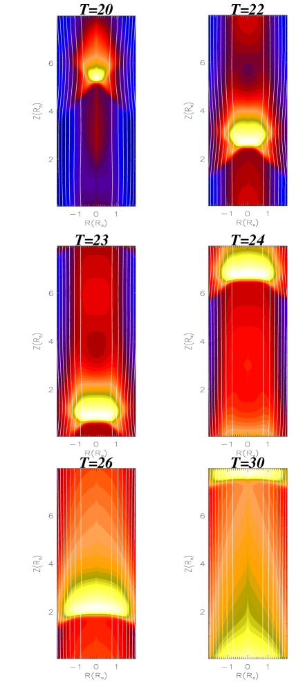
Figure 2: Temporal evolution (in $\tau_{o}$ unit) of a typical internal shock occurring within the jet. The grey-scales represent density levels (dark for low density and white for high density) while solid lines stand for poloïdal magnetic field lines. The parameters of this simulations are $\beta_{p}=10$, $M_{o}=10$, $R_{c}=1$ and $\delta M_{o}=0.1$. This shock arises from a initial setup prone to axisymmetric MHD Kelvin-Helmholtz instabilities. In the early stage of the shock evolution, the shock front displays a bow-shock shape but as the simulation goes on, the shock front evolves toward a front shock.

4.2.3 Inner-jet shock evolution

Kelvin-Helmholtz instability is believed to be one of the source of flow perturbation in astrophysical jets. The evolution of this mechanism has been widely investigated either in a hydrodynamical framework (e.g. Micono et al. (2000) and reference therein) or more recently using MHD framework (see Baty & Keppens (2002) and reference therein). The growth and formation of shock as well as vortices in the jet core depend on the nature of the jet (magnetized or not) and on the magnetic field strength (Malagoli et al., 1996; Frank et al., 1996; Jones et al., 1997; Keppens & Tóth, 1999). In the particular case of axisymmetric jets, it has been shown that the presence of a weak magnetic field significantly modifies the evolution of the inner structures of vortices.
We present on Fig. 2 the temporal evolution of a typical inner-jet shock obtained from our computations. After the linear growth of the instability (up to $t=19\tau_{o}$), the structure exhibits a curved front shock inclined with respect to the jet axis. In the frame of the shock, the flow is upstream super-fastmagnetosonic, and downstream sub-fastmagnetosonic. On both side of the shock, the plasma flow remains superalfvènic. This shock configuration is consistent with a super-fast shock. Rankine-Hugoniot relations show that, at a fast-shock front, the magnetic field component parallel to the shock front is larger in the downstream medium than in the upstream one (Fraix-Burnet & Pelletier, 1991). In the present axisymmetric simulations, the bending of the poloïdal magnetic field lines occurring at the shock front creates a locally strong Lorentz force that tends to push the structure out of the jet. As seen on the following snapshots of Fig.2, the shock front rapidly evolves toward a plane shape. This quasi-plane shock structure remains stable for several time units before being diluted.

4.2.4 Macroscopic quantities

The SDEs coupled with the MHD code provide approximate solutions of the Fokker-Planck equation using macroscopic quantities calculated by the MHD code. Indeed, flow velocity and magnetic field enter the kinetic transport equation and there is no way to treat realistic case in astrophysical environments but to model them from macroscopic multi-dimensional simulations. Nevertheless, one difficulty remains since MHD (or HD) simulations only give these macroscopic quantities values at discrete location, namely at each cells composing the numerical mesh. Hence, these values are interpolated from the grid everywhere in the computational domain. If the domain we are considering is well-resolved (large number of cells in each direction), a simple tri-linear interpolation is sufficient to capture the local variation of macroscopic quantities. When shocks are occurring, the sharp transition in velocity amplitude is more difficult to evaluate because shocks are typically only described by few cells. Thus, the calculus of velocity divergence must be done accurately. We adopt the following procedure to calculate it: shocks are characterized by very negative divergence so at each cells $(i,j)$ we look for the most negative result from three methods

$$\nabla\cdot{\bf u}(i,j)=min\left(\mp\frac{u_{Z}(i,j)-u_{Z}(i,j\pm 1)}{|Z(j)-Z(j\pm 1)|},\right.$$ (36)

$$\left.\frac{u_{Z}(i,j+1)-u_{Z}(i,j-1)}{Z(j+1)-Z(j-1)}\right)$$

$$+ \min\left(\mp\frac{R(i)u_{R}(i,j)-R(i\pm 1)u_{R}(i\pm 1,j)}{R(i)(R(i)-R(i\pm 1))},\right.$$

$$\left.\frac{R(i+1)u_{R}(i+1,j)-R(i-1)u_{R}(i-1,j)}{R(i)(R(i+1)-R(i-1,j))}\right)$$

This approach ensures that the sharp velocity variation occurring within a shock is well described and that no artificial smoothing is created in the extrapolation of flow velocity divergence. At last, note that the location of the most negative $\nabla\cdot{\bf u}$ corresponds to the shock location. The measurement of spectra at shock front will then be done by looking at particles characteristics passing through this location.

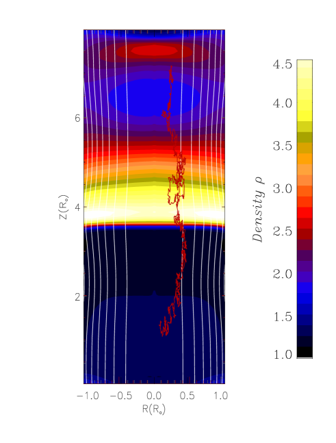
Figure 3: Zoom in a jet snapshot where Kelvin-Helmholtz instabilities are active. The parameters of the MHD simulations are the same as in Fig.2. The grey levels represent the density levels while the white lines are magnetic surfaces. A shock arises in the core of the jet ($R\leq 1$) with a plane shape perpendicular to the jet axis. Using a large number of particles like the one which trajectory is displayed with a thick white line, we measure, in the shock frame, the stationary energetic spectrum of particles at the shock front.

Figure 4: Energetic spectrum of particle population injected at momentum $p_{o}$ in the MHD jet of Fig. 3. The spectrum is measured at the shock front and is in a very good agreement with DSA theory predicting a power-law of index $-4$ for a single plane shock of compression ratio $r=4$. Note that in this computation the diffusion coefficients have constant values fulfilling relation (17).

4.3 Realistic plane shock

In this subsection we address the issue of the production of energetic spectra by plane shocks arising from MHD simulations. This issue is a crucial test for the relevance of SDEs using the velocity divergence defined in Eq.(36). We stress that all simulations performed in this paper are done using test-particle approximation, i.e. no retroactive effects of the accelerated particles on the flow are taken into account.

4.3.1 Strong shock energetic spectrum

We have performed a series of MHD simulations of cylindrical jets subject to Kelvin-Helmholtz instabilities (cf. Sect. 4.2). We selected the case of a plane shock (quite common in the KH instability simulations) propagating along the jet with a radial extension up to the jet radius (see Fig. 3). Its compression ratio is $r=4$ (measured by density contrast) and constant along the shock front. We have chosen a particular snapshot of the structure displayed on Fig. 3. By rescaling the vertical velocity in order to be in the shock frame (where the down and up-stream velocities are linked by $u_{\rm{down}}=u_{\rm{up}}/r$), we first consider this shock with infinite vertical boundaries and reflective radial boundaries. Namely, we set that if the particle is escaping the domain at $Z<Z_{min}=0$ or $Z>Z_{max}=8$, we take the velocity to be ${\bf u}_{p}(Z>Z_{max})={\bf u}_{p}(R,Z_{max})$ (same thing for $Z<Z_{min}$). The condition allows for particles far from the shock to eventually return and participate to the shaping of $F(p)$. The reflective radial boundaries are located at the jet axis $R=0$ (to avoid the particle to reach $R=0$ where SDEs are not valid) and $R=1$. Such boundaries ensure that no particle can radially escape from the jet during the computation. The constant value of the diffusion coefficients $D_{ZZ}$ and $D_{RR}$ must fulfill relations (17) and (19). Actually, in the particular case of a plane shock propagating along the vertical axis, only $D_{ZZ}$ must fulfill previous relations, namely $D_{ZZ}>D_{min}=X_{sh}|u_{Z}|/2$. The shocks width $X_{sh}$ is defined as the location of the most negative velocity divergence of the flow. Typically, this width corresponds to the size of a mesh cell in the case of strong shock. We can then safely set $D_{ZZ}=0.4$ as we will have $D_{ZZ}=10D_{min}$. The radial diffusion coefficient is tuned as $D_{RR}=0.01$ and will enable particle to explore the shock front structure. On Fig. 4 we display the results of the use of SDEs on a particle population injected at momentum $p=p_{o}$ and propagating in snapshot represented by Fig. 3. We easily see that the resulting spectrum is a power-law of index $-4$ completely in agreement with DSA theory (see Section 2). The existence of a few particle with $p<p_{o}$ arises from the fact that outside the shock, the velocity divergence is not equal to zero, as it would be with a prescribed velocity profile (Krülls & Achterberg, 1994; Marcowith & Kirk, 1999). Note that in the absence of other energetic mechanism (as second-order Fermi acceleration or synchrotron losses), the simulation is independent of the physical value of $p_{o}$ as the diffusion coefficient is independent of $p$.

4.3.2 Single shock with synchrotron losses

Figure 5: Energetic spectrum of energetic population injected at momentum $p_{o}c=100MeV$ in the MHD jet of Fig. 3 and subject to synchrotron emission. The spectrum is measured at the shock front. It matches the solution of Webb et al. (1984), in particular for the cut-off momentum $p^{*}$ where synchrotron losses balance shock energy gains. For this computation, we have considered magnetic field given by the MHD code. The upstream velocity $U_{up}=300\rm{km/s}$, and the mean magnetic field $B_{o}=100\ \rm{\mu G}$.

For electrons, the acceleration occurring within shock may be balanced at the cut-off by radiative losses due to the presence of the jet magnetic field. Webb et al. (1984) has presented a complete analytical resolution of Fokker-Planck transport equation including both first-order Fermi acceleration and synchrotron emission. In particular, they show that the energetic spectrum exhibits a cut-off at a momentum $p^{*}$ depending on spatial diffusion coefficient and velocity of the flow. The choice of the injection energy $p_{o}c$ of electrons is determined by the lower boundary of the inertial range of magnetic turbulence. Indeed, to interact with turbulence and to spatially diffuse, electrons must have momentum larger than $p_{i}=m_{i}V_{A}$, where $m_{i}$ is typically the proton mass and $V_{A}$ is the Alfvén speed (Lacombe, 1977). The energy threshold corresponds to

$$\epsilon_{i}=p_{i}c\simeq 900MeV\left(\frac{V_{A}}{c}\right)$$ (37)

In our simulations, we assume an Alfvèn speed $V_{a}\sim 2.2\ 10^{8}\ \rm{cm/s}\sim c/100$ (see the discussion in Section 2.2) leading to $p_{o}c=100MeV\geq p_{i}c$. As previously noted, the Alfvèn speed in extragalactic jets can reach appreciable fraction of the light speed. An increase of $V_{a}$ leads to an increase of the particle injection threshold and a decrease of the dynamical momentum range explored. In that case, the Fermi second order effect must be included in our SDE system (via the diffusive term in momentum in Eq. 15). Time dependent simulations (in progress) will include the associated discussion.
The result of the simulation including synchrotron losses is displayed on Fig. 5. When assuming a constant magnetic field and diffusion coefficients, the cut-off energy $\epsilon^{*}=p^{*}c$ reads as (Webb et al., 1984)

$$\epsilon^{*} = \frac{m_{e}^{2}c^{3}}{D_{ZZ}}\frac{2\pi}{\sigma_{T}B^{2}}u_{\rm{up}}^{2}\frac{r-1}{r(r+1)}$$ (38)

$$= 0.48GeV\left(\frac{U_{\rm{up}}}{300km/s}\right)\left(\frac{R_{jet}}{100pc}\right)^{-1}\left(\frac{B}{100\mu G}\right)^{-2}$$

Fig. 5 displays the spectrum at the shock in case of a the magnetic field obtained from the MHD code. The cut-off is in good agreement with the resulting spectrum despite the numerical simulation is considering a spatially varying magnetic field. The Fig.  5 also shows the case of a constant magnetic field taken as the average of the previous one.

Figure 6: Energetic spectrum resulting from acceleration by multiple shocks in an extragalactic jet. The power-law arising from this simulation matches exactly the result given by DSA theory in the case of no particle escape from the shock region ($t_{esc}\gg t_{acc}$). To achieve this simulation, we have considered the snapshot in Fig.3 but with vertical re-injection of escaping particles. These boundaries mimic the effect of multiple shocks interaction with particle during their propagation along the jet.

4.3.3 Multiple shocks acceleration

The presence of multiple shocks increases the efficiency of particle acceleration. In multiple shocks, the particles accelerated at one shock are advected downstream towards the next shock. The interaction area is enhanced, so as the escaping time. The general expression of the distribution function at shocks front, $\log f\propto-(3+t_{acc}/t_{esc})\log p$ will then tend to $\log f\propto-3\log p$. This multiple shocks acceleration may occur in jets where numerous internal shocks are present (Ferrari & Melrose, 1997). We intend to modelize this effect using the same snapshot as in previous calculations but changing the nature of the vertical boundaries. Indeed, since we are modelizing only a small part of the jet (typical length of $800pc$), we can assume that if a particle is escaping by one of the vertical boundaries, it can be re-injected at the opposite boundary with identical energy. The re-injection mimics particle encounters with several parts of the jet where shocks are occurring. Physical quantities are set to same values than in paragraph dealing with single plane shock. The result of the simulation is displayed on Fig. 6 and on Fig. 7 when synchrotron losses are considered. On Fig. 6, the spectrum reaches again a power-law shape but with a larger index of $-3$, consistent with previous statements. When synchrotron losses are included in SDEs (Fig. 7), we find a similar spectrum than for single shock but with some differences. Namely, the curve exhibits a bump before the cut-off. This bump can easily be understood since the hardening of the spectrum enables particles to reach higher energies where synchrotron losses become dominant. Thus an accumulation of particles near the cut-off momentum $p^{*}$ will occur. The bump energy corresponds to the equality between radiative loss timescale and multiple shock acceleration timescale. The last timescale is larger than the timescale required to accelerate a particle at one isolated shock because of the advection of particles from shock to next one (Marcowith & Kirk, 1999).

Figure 7: Momentum spectrum of electrons injected at $p_{o}c=100MeV$ in a jet prone to multiple shocks acceleration. Note the bump occurring because of the synchrotron cut-off that tends to accumulate particles at the cut-off momentum $p^{*}$.

Figure 8: Spectrum produced by plane shocks with spatially varying compression ratio $r$. The left panel represents compression ratio profiles along the shock front while the right panel displays the resulting spectra. The calculations 1, 2 and 3 have different $r-$profiles but the same $r_{m}=4$. The resulting spectra are corresponding to curve 1,2 and 3 on the right figure. We can see that this curves are almost the same and are very close to a power-law with index $-(r_{m}+2)/(r_{m}-1)$. Curves 4 and 5 correspond to compression ratio profile with mean values $r_{m}$ equal to $3.5$ and $3$. The corresponding spectra on the right figure are again consistent with power-law with indices controlled by their $r_{m}$. All particles are injected at $p_{o}c=100\ \rm{MeV}$ along the shock.

5 Acceleration at complex shock fronts

The shock structures are subject to important evolution during the development of the KH instability. We now investigate the particle distribution function produced at these shocks using the SDE formalism. All the shock acceleration process here is investigated using snapshots of the MHD flow.

5.1 Plane shocks with varying compression ratio

In astrophysical and particularly jet environments, (weak) shocks occurring within magnetized flows in the early phase of KH instability (see Fig. 2) are non-planar and/or with non-constant compression ratio along the shock surface. We first consider analytical calculations of the particle distribution produced in such shocks that extend previous works and we complete our estimates using the MHD-SDE system.

5.1.1 Analytical approach

The theory of DSA explains the energetic spectrum of diffusive particles crossing plane shock with constant compression ratio $r$. Even when the plane structure is relaxed (Drury (1983)) the compression ratio is usually assumed as constant along the shock front. In astrophysical jets, complex flows arise from the jet physics so that even the plane shock assumption is no longer valid implying a non-analytical derivation of the particle distribution function. Nevertheless, it seems obvious that if the shock front is not strongly bent, the particle acceleration process should not be strongly modified.
Let us first quantify this assertion. We calculate the mean momentum gained by a particle during one cycle (downstream $\rightarrow$ upstream $\rightarrow$ downstream)

$$\frac{<\Delta p>}{p}=\frac{4}{3}(r(R)-1)\frac{u_{d}}{v}$$ (39)

we assume that, during this cycle, the particle sees the local structure of the shock as a plane ($v$ is the speed of the particle), e.g. the spatial scale where the shock bends is large compared to the particle diffusive length.
Here, contrary to the standard DSA theory, the energy gain depends on the location of the shock crossing of the particle. The probability for a particle to escape from the shock during one acceleration cycle is however still given by the usual DSA theory, namely $\eta_{k}=4u_{d}/v_{k}$ ($v_{k}$ is the speed of the particle during the $k$th cycle). The probability that a particle stays within the shock region after $n$ cycle $Pr_{n}$ can be linked to the mean momentum gain after $n$ cycle as

$$\frac{\ln{Pr_{n}}}{\ln{p_{n}/p_{o}}}=\frac{\sum_{k=1}^{n}\ln(1-\eta_{k})}{\sum_{k=1}^{n}\ln(1+\eta_{k}(r_{k}-1)/3)}\ .$$ (40)

The compression ratio $r$ depends on the number of the cycle since in reality, the particle is exploring the front shock because of the diffusion occuring along the shock front. This expression can be simplified if we assume the flow background velocity very small compared to particle velocity ($\eta_{k}\ll 1$ for a non-relativistic shock) and that particles are ultra-relativistic ($\eta_{k}=\eta=4u_{d}/c$). The expression then becomes

$$\frac{\ln{Pr_{n}}}{\ln{p_{n}/p_{o}}}\simeq-3\frac{n}{\sum_{k=1}^{n}r_{k}-n}\ .$$ (41)

The sum of the different compression ratios experienced by particle population can be approximated using the average compression ratio measured along the shock front $r_{m}$. Indeed, each particle interacting with the shock are prone to numerous cycles of acceleration and then the sum remaining in Eq.(41) can be expressed as $\sum_{k=1}^{n}r_{k}\simeq nr_{m}$. Hence, the energetic spectrum is a power-law but with an index controlled by the mean value of the compression ratio all over the shock front, namely

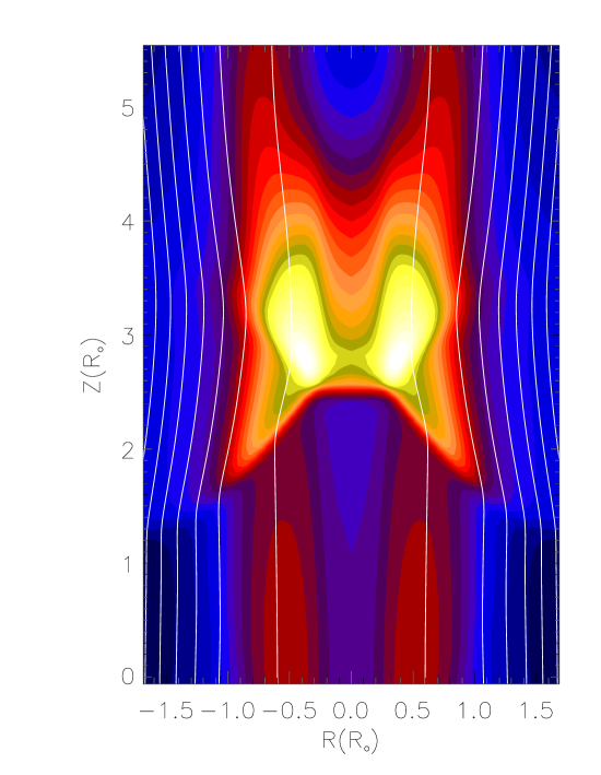
Figure 9: Same plot as Fig.(3). The MHD simulation parameters are the same as in Fig.3 except for $\delta M_{o}=0.5$. This snapshot is selected during the developing phase of the shock where the structure is evolving toward a plane shock. The inclined (with respect to the jet axis) part of the shock front are affected by a strong magnetic bending due to magnetic conservation through the shock.

$$p^{2}f\propto\frac{\partial\ln Pr_{n}}{\partial p_{n}}\propto p^{-3(r_{m}+2)/(r_{m}-1)}\ .$$ (42)

In this demonstration, the compression ratio profile itself is not involved in the spectrum shape but only its average value $r_{m}$, as long as one can consider the shock to be locally plane. Eq.(42) generalizes the results provided by Drury (1983) concerning curved shocks with constant compression ratio. If the plane shock assumption is relaxed, numerical simulations are necessary.
In order to complete this result, we have performed several numerical calculations where a mono-energetic population of relativistic particles are injected with momentum $p_{o}$ behind an analytical prescription describing a plane shock with varying compression ratio (the shocks are test examples). The result of this numerical test is displayed on Fig.(8).
In this test, we have done three calculations with three different compression ratio profiles (curves 1, 2 and 3) but with identical average value $r_{m}=4$. Setting both vertical and radial diffusion, we have obtained the spectra 1, 2 and 3 displayed on right panel of Fig.(8). These three curves are almost the same. On two other calculations, we have chosen linear profiles with different values of $r_{m}$ (curves 4 and 5): again a power-law spectrum is found with indices consistent with previous analytical statements. This conclusion is correct only if during on cycle the particle mean free path along the shock front is small compared to its curvature and if during many cycles the particle is able to explore the whole shock structure.

5.1.2 Locally-plane shock

The previous considerations can be applied to a non-planar shock produced in the early stage of the axisymmetric Kelvin-Helmholtz instability. The inner shocks tend to evolve from curved fronts in the early phases of the instability toward plane shocks, perpendicular to the jet axis (see Sect.4.2.3 and Fig.2). On Fig.9 the curvature radius of the shock is typically of the order of the jet radius while the obliquity angle (between the shock front and the jet axis) ranges from zero to $27^{o}$. For such a low obliquity the shocks are subluminal. A more subtle consequence of the non-constancy of the compression ratio is that the electric fields generated along the shock front cannot be canceled by any Doppler boost. In other words, complex shocks do not have a unique de Hoffman-Teller frame. This problem strongly complexifies the particle acceleration and transport in jets and is postponed to future works especially treating strongly oblique (or even perpendicular) shocks. In the present paper, the MHD shocks are only weakly oblique and non-relativistic (the effects of electric fields on particle acceleration are neglected). In principle, once the electro-magnetic field is known throughout the jet, the systematic electric effects on particle trajectories can be implemented in the SDE system.
Keeping the same prescription for diffusion coefficients than in previous section (constant diffusion coefficients and radial reflective boundaries) we first have to verify the quasi-planar condition of the shock. To this aim, we form the ratio of the typical diffusion length occurring during one cycle along the shock front ($L_{\perp}$) and the curvature radius. The duration of one acceleration cycle is controlled by the residence time at the shock $t_{res}=2D_{ZZ}/u^{2}_{d}$ (assuming that it is composed of $n$ identical cycle). The number of cycle needed for the particle to escape the shock is obtained when the escaping probability after $n$ cycles is equal to unity, namely $\sum_{k=1}^{n}\eta_{k}=4nu_{d}/c$ when particles are relativistic. The duration of one cycle is thus $\tau=8D_{ZZ}/u_{d}c$. The criterion for considering a shock as locally plane will be

$$\frac{L_{\perp}}{L_{curv}}\leq\frac{\sqrt{2D_{\perp,S}\tau}}{R_{jet}}$$ (43)

where $D_{\perp,S}$ is the maximal value of the diffusion coefficient in the direction parallel to the shock front. With the previously prescribed diffusion coefficients the ratio has a maximum value equal to $3.4\ 10^{-2}$. This value is small compared to unity which means that during one cycle, the particle will interact with a zone of the shock where the compression ratio is almost constant. On the other hand, this ratio is not so small and within a few cycles of acceleration particles will explore a significant part of the shock front.
Figure(10) shows the energetic spectrum produced in such curved shock. The result is close to a power-law of index $f\propto p^{-4.7}$ and when synchrotron losses are taken into account, the cut-off energy corresponds to the case of a uniform shock with constant compression ratio equal to $2.76$. The cut-off, given by Eq.(38) is close to the value obtained on the plot. We postpone to Section 5.2.2 the comparison between particle acceleration timescale and shock survival timescale in the different phases of the jet evolution. We can however anticipate here that for typical jet parameters the former is smaller than the latter. This validates our results obtained using MHD snapshots.

Figure 10: Compression ratio profile (left) and energetic spectrum (right) of accelerated particles by the shock displayed on Fig.9. This shock is not a plane shock and does not have constant compression ratio along its shock front. The curvature radius of this shock is much larger than the mean free path of a particle so, locally, the shock can be considered as a plane shock. The resulting spectra (with only acceleration or with synchrotron losses included) are consistent with a plane shock with compression ratio $2.7$ which is close to the average value of the compression ratio of this shock, namely $r_{m}=2.68$.

5.2 Strong shock acceleration and spatial transport

We now consider the shock acceleration and spatial transport in chaotic magnetic field in strong shocks occurring in the late phase of the KH instability where the most efficient particle acceleration is expected (Micono et al., 1999). The validity of the snapshot approach is tested against the survival of the shocks. We investigate the effect of radial escape on the particle distribution in the single and the multiple shock configuration.

5.2.1 Maximum energies expected and electron transport

The maximum electron energy is limited by radiative or escape losses. In case of synchrotron radiation, the loss timescale is $\tau_{\rm{loss}}\sim 1.2\ 10^{4}(B_{\rm{mG}})^{-2}\ E^{-1}_{GeV}\ \rm{yr}$ which compared to the acceleration timescales presented above leads to electron with energies $\gamma_{max}\sim 10^{8}\ (U_{jet}/c)^{3/2}$, around 1 TeV for $U_{jet}/c=0.1$ (the magnetic field and the particle energy are expressed in mGauss and in GeV units respectively).
In a quite general way, the radial and vertical diffusion coefficients can be written as

$$D_{RR} = D_{\parallel}\left|\frac{B_{R}}{B}\right|+D_{\perp}\left(1-\frac{B_{R}^{2}}{B^{2}}\right)^{1/2}$$

$$D_{ZZ} = D_{\parallel}\left|\frac{B_{Z}}{B}\right|+D_{\perp}\left(1-\frac{B_{Z}^{2}}{B^{2}}\right)^{1/2}$$ (44)

where $B$ is the total magnetic field amplitude. The confinement time is driven by the radial diffusion coefficient $D_{RR}$ which may be expressed in term of $\eta_{T}$ as

$$D_{RR}\simeq\frac{D_{o}}{\eta_{T}}(\alpha+(1-\alpha^{2})^{1/2}\eta_{T}^{2.3})\ ,$$ (45)

where $D_{\parallel}=D_{o}/\eta_{T}$ and $\alpha$ stands for the average value of $|B_{R}/B|$ all over the simulation box. The coefficient $D_{o}$ may eventually depends on the particle momentum. It can easily be seen that Eq.(45) has a minimum value for

$$\eta_{T}^{min}=\left(\frac{\alpha}{1.3\ (1-\alpha^{2})^{1/2}}\right)^{1/2.3}\ .$$ (46)

At $\eta_{min}$, particle confinement reaches its maximum (see Eq. 22). Typically, radio jets do not display opening angle larger than a few degrees leading to $\eta_{T}^{min}$ of the order of $0.2$. Paradoxically, low turbulence levels do not provide efficient confinement since largest diffusion motion occurs along the magnetic field which have locally radial components. Within a timescale $\tau_{loss}$ electrons are able to explore distances

$$\Delta R=\sqrt{4\ D_{RR}\ \tau_{loss}}\ .$$ (47)

In the chaotic magnetic regime, Eq.(3) leads to

$$\Delta R\sim 15\ [\frac{(\alpha+(1-\alpha^{2})^{1/2}\eta_{T}^{2.3})}{\eta_{T}}]^{1/2}\ E_{\rm{GeV}}^{-1/3}\ B_{\rm{mG}}^{-7/6}\ \rm{pc}.$$ (48)

We consider a mean turbulence level $\eta_{T}=\eta_{T}^{min}$, and assumed a magnetic field $B=100\ \rm{\mu G}$, and a maximum turbulence scale $\lambda_{max}\sim R_{\rm{jet}}$. For $\alpha\sim 2^{o}$, we get $\Delta R(\rm{1\ TeV})\sim 9\ \rm{pc}$ and $\Delta R(\rm{1\ GeV})\sim 90\ \rm{pc}$. The high energy electrons are only able to explore about one tenth of the jet radius and can be considered as confined to the region where they have been injected. The GeV electrons can explore larger fraction of the jet and escapes are expected to steepen the particle distribution. These are averaged results, $\Delta R$ is sensitive to the magnetic field, for example if B decreases (increases) by one order of magnitude $\Delta R$ increases (decreases) by a factor $\sim 14$. Along the jet, particles are advected from one shock to the next on timescales $\Delta Z_{shock}/V_{flow}$, where a mean inter-shock distance $\Delta Z_{shock}\sim 1\ \rm{kpc}$ and $V_{flow}\sim 10^{-2/-1}c$ lead to $\tau_{adv\parallel}\sim 3\ 10^{4/5}\rm{yr}$. The high energy part of the electron distribution is then produced by one shock and can hardly be re-accelerated in a second one downstream. The spectrum at these energies strongly depends on the shock compression ratio. At lower energies GeV electrons distribution can be subject to either transversal escapes or multiple shock effects. For both populations, the electrons accelerated at inner shocks remain within 1 kpc from their injection points, this clearly separates the inner jet to the Mach disc and justifies a fortiori our approach simulating only the kiloparsec scale jet. It also clearly appears that the spatial transport issue addresses to the multi-wavelength morphologies of jets. We know make these statements more precise using the coupled MHD-SDE system.

5.2.2 Single shock

So far, we have presented numerical calculations using reflective radial boundaries (no particle losses) and constant diffusion coefficients. In this section, we choose to remove step by step these two constraints. Starting from the snapshot of Fig.3, we first remove the outer reflective boundary and consider any particle having $R>R_{jet}$ as lost. Then we adopt diffusion coefficients given by Eq. (3) since they arise from a transport theory consistent with high turbulence levels $\eta_{T}$ and are confirmed numerically. Quasi-linear theory does likely apply at very low turbulence levels implying high parallel diffusion coefficient and acceleration timescales. Expected spectra must then be softer than the same spectrum obtained in chaotic regime.
First, as an illustration of escape effects, we consider the case of constant diffusion coefficients, namely $D_{ZZ}=1$ and $D_{RR}=2.10^{-2}$. The resulting spectrum can be seen on Fig.11 and is consistent with a harder power-law. In previous simulations, the escaping time was defined as the time needed by the flow to advect a majority of RPs away from the shock. Here the effect of the confinement inside the jet if lower than the escaping time from the shock will be the main source of particle losses. The distribution function reads as $\log{f}\propto-(3+t_{acc}/t_{loss})\log{p}$ where $t_{loss}=min(t_{conf},t_{esc})$ and will stay as a power-law as long as the escaping time is not momentum dependent. In our example $t_{loss}=t_{conf}=(R_{jet}-R_{inj})^{2}/4D_{RR}=10.125$, where $R_{inj}$ is the average radius of injected particles. The resulting spectrum index on Fig.11 is in good agreement with this estimate since the ratio $t_{acc}/t_{conf}=6D/(t_{conf}u_{d}^{2}(r-1))=1.26$ and the plot representing the spectrum done with these constant diffusion coefficients has a power-law index as $f\propto p^{-4.25}$.
Secondly, we discuss the case of Kolmogorov turbulence and keep $\eta_{T}$ free in order to check its influence on the transport of particles. The three last plots in Fig.11 represent simulations performed without outer reflective boundaries and diffusion coefficients as described by Eq.44. The simulations account for energy as well as spatially ($B_{r}$ and $B_{z}$ are both function of r and z) dependent transports. Each curve corresponds to a value of the turbulence level $\eta_{T}=0.05,0.2$ and $0.9$. In a Kolmogorov turbulence $D_{\parallel}\propto D_{\perp}\propto p^{1/3}$, $t_{conf}\propto D_{RR}^{-1}\propto p^{-1/3}$ which leads to a confinement time decreasing while increasing momentum and a convex spectrum. At a low turbulence level, the ratio $t_{acc}/t_{conf}$ is large, increases with the particle momentum and leads to softer spectra with low energy cut-off (at few GeV/c). In order to get significant particle acceleration and large energy cut-off (beyond 1 TeV) turbulence levels $\eta_{T}\geq 0.1$ seem mandatory. The maximum confinement is obtained for turbulence level $\eta_{T}$ compatible with Eq. (46).

Figure 11: Spectra produced at the shock front displayed on Fig.3 without outer reflective boundary, namely with radial particle losses. The upper plot represents a spectrum done with constant diffusion coefficients ($D_{ZZ}=1$ and $D_{RR}=0.02$). The radial losses modify the spectrum by increasing the index of the power-law from $-4$ to $-4.25$. The last three curves are spectra produced by using realistic diffusion coefficients given by Eq.(3). The momentum dependence of these coefficients modifies the shapes that are no longer power-laws (see Sect.5.2.2). The upper plot has an arbitrary normalization unrelated to the three last curves.

One important issue to discuss about is the validity of our results while considering snapshots produced from the MHD code. It appears from Fig. 2 that both weak curved and strong plane shocks survive a timescale of the order of $5\ \tau_{o}$. The shock acceleration timescale of a particle of energy $E_{\rm{GeV}}$ may be expressed as $\tau_{acc}\sim 20\ D_{ZZ}/U^{2}_{\rm{sh}}$ for a compression ratio of 4 (Drury, 1983), where $U_{\rm{sh}}\sim 10\ c_{s}$ is the shock velocity. Using the Eq. 3) and 44 we end up with a typical ratio $\tau_{acc}/\tau_{0}\sim 10^{-2}\ \eta_{T}^{-1}\ E^{1/3}_{\rm{GeV}}\ B^{-1/3}_{mG}$. Our snapshot then describes well the shock acceleration (e.g. $\tau_{acc}/\tau_{0}\leq 1$) up to TeV energies unless the turbulence level is very low and the magnetic field much lower than $100\mu G$. The conclusion is the same for curved shocks as the acceleration timescale is smaller in that case. However, time dependent simulations are required to a more exhaustive exploration of the jet parameter space and to test the different turbulence regimes.

5.2.3 Multiple shock-in-jet effects

Figure 12: Same plot as in Fig.11 but with periodic vertical boundaries. This setting mimics the effect of multiple shocks acceleration. As previously, inclusion of radial particle losses affects spectra: a softening of the spectral index, cut-off energies dependent on $\eta_{T}$.

The radial losses should also affect the transport of particles encountering several shocks during their propagation. This description is pending to the possibility of multiple strong shocks to survive few dynamical times. This issue again requires the time coupling between SDE and MHD simulations to be treated.
However, the general statement about the distribution function is still valid but at the opposite of previous multiple shocks acceleration calculations (see Section 4.3.3) the lack of confinement is the only loss term. On Fig.12, we have performed the same calculations as in the previous paragraph except that we impose periodic vertical boundaries where particles escaping the computational domain by one of the vertical boundary is re-injected it at the opposite side keeping the same energy.
We again start with our fiducial case displaying the spectrum obtained from calculations done with constant diffusion coefficients, i.e. $D_{ZZ}=1$ and $D_{RR}=2\ 10^{-2}$ (the upper plot). The power-law index is modified and equals to $-3.13$ instead of $-3$ as obtained in calculations without radial losses. This result is close to the analytic estimate since $t_{acc}/t_{conf}\simeq 0.11$ in that case. In the chaotic diffusion regime the same behavior is observed in the spectra, e.g. convex shape, low energy cut-off at low turbulence levels. In this diffusion context, multiple shock acceleration is again most efficient for $\eta_{T}\sim 0.2-0.3$ and tends to produce hard spectra up to 10-100 GeV for electrons without radiative losses. The spectrum cut-off beyond 10 TeV.
In Fig.13, we have included synchrotron losses effects in one of the most favorable case ($\eta_{T}=0.25$) in the chaotic regime. The resulting spectrum shows a characteristic bump below the synchrotron cut-off lying around a few ten GeV. This hard spectrum may be intermittent in jets as already noticed by Micono et al. (1999). The spectrum and bump may also not exist because of non-linear back-reaction of relativistic particles on the shock structure (this problem require the inclusion of heavier particles in the simulation). Beyond the electrons loss their energy before reaching a new shock as discussed in Section 5.2.1. The magnetic field used is $10\ \mu G$ and suggests that higher values are apparently not suitable to obtain TeV electrons. The synchrotron peaked emission of the most energetic electrons of this distributions gives an idea of the upper limit of radiative emission achievable by this inner-jet shock. In a $10\mu G$ magnetic field, these electrons radiate UV/X-ray photons as (Rybicki & Lightman, 1979)

$$h\nu_{syn}=0.29\frac{3h\epsilon^{2}eB}{\mu_{o}m^{3}_{e}c^{5}}\sim 20eV\left(\frac{\epsilon}{10TeV}\right)^{2}\left(\frac{B}{10\mu G}\right)$$ (49)

The electron population computed here does not go beyond $50\ \rm{TeV}$, which then suggests an energy emission upper limit around $\sim 0.5\rm{keV}$. The maximum energy scales as $U_{jet}$ (see Eq.(38)) and can be significantly increased in case of fast jets (with speeds up to c/2 the limit of the validity of the diffusion approximation).
In case of inefficient confinement, e.g. $\eta_{T}$ different from 0.2-0.3, this result also suggests that the synchrotron model may in principle not account for the X-ray emission of extragalactic jets probably dominated by another radiative mechanism (for instance the Inverse Compton effect). However again, we cannot draw any firm conclusions about this important issue and postpone it to the next work treating full time dependent simulations.

Figure 13: Multiple inner-jet shocks spectrum including synchrotron losses for $\eta_{T}=0.2$, $B_{o}=10\mu G$ and $U_{jet}=c/5$. The synchrotron cut-off energy lies at a few $TeV$. The most energetic electrons at the bump of this distribution would have a peaked synchrotron emission at $\nu\sim 1.9\ 10^{16}Hz$ which corresponds to UV/X-ray emission ($h\nu\sim 20eV$).

6 Concluding remarks and outlook

In the present work, we performed 2.5D MHD simulations of periodic parts of extragalactic jets prone to KH instabilities coupled to a kinetic scheme including shock acceleration, adiabatic and synchrotron losses as well as appropriate spatial transport effects. The particle distribution function dynamics is described using stochastic differential equations that allow to account for various diffusion regimes.
We demonstrate the ability of the SDEs to treat multi-dimensional astrophysical problems. We pointed out the limits ($D_{min}$ defined in Eq. 19) imposed by the spatial resolution of the shock on the diffusion coefficient. The SDEs are applicable to particular astrophysical problem provided $D\geq D_{min}$. We perform different tests in 2D showing consistent results between numerical simulations and analytical solutions of the diffusion-convection equation. Finally we demonstrate the ability of the MHD-SDE system to correctly describe the shock acceleration process during the evolution of the KH instability. Complex curved shock fronts with non constant diffusion coefficients that occur at early stage of the instability behave like plane shock provided the diffusion length is smaller than the shock curvature. The equivalent plane shock has a compression ratio equals to the mean compression of the curved shock. In case of strong plane shocks which develop at later stages of the KH instability, we found that the inclusion of realistic turbulent effects, e.g. chaotic magnetic diffusion lead to complex spectra. The resulting particle distributions are no more power-laws but rather exhibit convex shapes linked to the nature of the turbulence. In this turbulent regime, the most efficient acceleration occurs at relatively high turbulence levels of the order of $\sim 0.2-0.3$. The electron maximum energies with synchrotron losses may go beyond 10 TeV for fiducial magnetic field values in radio jets of $\sim 10\mu G$ and the spectrum may be hard at GeV energies due to multiple shock effects.
However, in this work, SDEs were used on snapshots of MHD simulations neglecting dynamical coupling effects, preventing from any complete description of particle acceleration in radio jets. Such dynamical effects encompass temporal evolution of shock, magnetic field properties and particle distribution. The time dependent simulations will permit us to explore the parameter space of the turbulence and to critically test its different regimes.
The simulations have also been performed in test-particle approximation and do not account for the pressure in RPs that may modify the shock structure and the acceleration efficiency. This problem will be addressed in a particular investigation of shock-in-jet acceleration including heavier (protons and ions) particles. Nevertheless the present work brings strong hints about the ability of first order Fermi process to provide energetic particles along the jet. Our first results tend to show that synchrotron losses may prevent any electron to be accelerated at high energies requiring either supplementary acceleration mechanisms or other radiative emission processes to explain X-ray emission as it has been recently claimed. Future works (in progress) will account for these different possibilities.