Search for Relativistic Curvature Effects in Gamma-Ray Burst Pulses

Abstract

We analyze the time profiles of individual gamma-ray burst (GRB) pulses, that are longer than 2 s, by modelling them with analytical functions that are based on physical first principles and well-established empirical descriptions of GRB spectral evolution. These analytical profiles are independent of the emission mechanism and can be used to model both the rise and decay profiles allowing for the study of the entire pulse light-curve. Using this method, we have studied a sample of 77 individual GRB pulses, allowing us to examine the fluence, pulse width, asymmetry, and rise and decay power-law distributions. We find that the rise phase is best modelled with a power law of average index $r=1.31\pm 0.11$ and that the average decay phase has an index of $d=2.39\pm 0.12$. We also find that the ratio between the rise and decay times (the pulse asymmetry) exhibited by the GRB pulse shape has an average value of 0.47 which varies little from pulse to pulse and is independent of pulse duration or intensity. Although this asymmetry is largely uncorrelated to other pulse properties, a statistically significant trend is observed between the pulse asymmetry and the decay power law index, possibly hinting at the underlying physics. We compare these parameters with those predicted to occur if individual pulse shapes are created purely by relativistic curvature effects in the context of the fireball model, a process that makes specific predictions about the shape of GRB pulses. The decay index distribution obtained from our sample shows that the average GRB pulse fades faster than the value predicted by curvature effects, with only 39$\%$ of our sample being consistent with the curvature model. We discuss several refinements of the relativistic curvature scenario that could naturally account for these observed deviations, such as symmetry breaking and varying relative time-scales within individual pulses.

Introduction

The temporal structure of gamma-ray bursts (GRBs) varies drastically, with no apparent pattern among bursts. Of the $>$2704 GRBs detected by the BATSE instrument onboard the Compton Gamma Ray Observatory (CGRO) (Fishman et al., 1994), less than 10 $\%$ of the detected light-curve profiles can be categorized as being similar in overall shape or morphology, in that they comprise coherent structures, or pulses of radiation. It is generally believed that these pulses represent the fundamental constituent of GRB time profiles (light curves), and appear as asymmetric pulses with a fast rise and a slower decay, often denoted FRED ”Fast Rise and Exponential Decay” (see Figure 1). Each pulse is assumed to be associated with a separate emission episode, with complex GRBs being superpositions of several such episodes, of varying amplitude and intensity. Although the duration and amplitude of the FRED pulses vary considerably, the shape is the only recurring pattern that can be distinguished among the vast range of complex GRB light curves that have been observed.

The observed $\gamma$-ray pulses are believed to be produced in a highly relativistic outflow, an expanding and collimated fireball, based on the large energies and the short time scales involved. There are several possible mechanisms underlying the emission, although the commonly assumed scenario is that individual pulses are created, when shocks internal to the relativistic outflow, drain the kinetic energy and accelerate leptons which radiate. In this paper we base our discussion on this standard, fireball model, in which the $\gamma$-rays arise from the internal shocks at a distance of $R\sim 10^{13}-10^{17}$ cm from the initial source (Piran, 1999). In the context of the fireball model, the episodic nature of the outflow causes inhomogeneities in the wind to collide and thus create the shocks. The dominant emission mechanisms are most probably non-thermal synchrotron (Tavani, 1996; Lloyd & Petrosian, 2000)) and/or inverse Compton emission (Liang, Kocevski, Boettcher, 2003), but there have been other suggestions, for instance, thermal, saturated Comptonization (Liang, 1997). The simplest scenario here is to assume an impulsive heating of the leptons and a subsequent cooling and emission. Therefore, the rise phase of the pulse is attributed to the energization of the shell and the decay phase reflects the cooling of the energized particles.

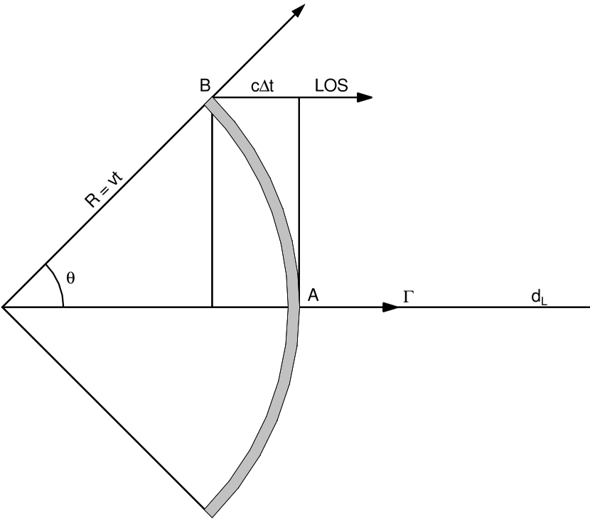
Figure 2: (a) Schematic drawing of the visible part of the fireball shell. The photons from A are boosted by 2$\Gamma$, whereas the photons from B are boosted by $\Gamma(1-\beta\cos{\theta})^{-1}$ and delayed by $\Delta t=R/c(1-cos{\theta}).$ Adapted from Ryde & Petrosian (2002).

As many authors have pointed out, this cooling interpretation does not work well when applied to non-thermal synchrotron and/or inverse Compton emission because the radiative cooling timescales alone are typically much too short to explain the pulse durations. For example, if we interpret the average break energy of a GRB spectrum ($\sim E_{pk}$) as the characteristic energy of synchrotron self-absorption, then the resulting magnetic field must be extremely high, about $1\times 10^{7}$ to $1\times 10^{8}$ Gauss. Similar estimates are obtained if we assume equipartition conditions between the lepton energy and the magnetic field. In either case, such a high $B$ field would create a synchrotron cooling timescale of the order of $10^{-5}$ seconds in the comoving frame (Wu & Fenimore, 1996). One resolution to this problem is to introduce relativistic effects. If the relativistic fireball expands with a Lorentz factor of $\Gamma$ $>$ 100, then the geometry of the shell would make radiation emitted off the line of sight delayed and affected by a varying Doppler boost (see Figure 2). This would cause the GRB spectra to evolve to lower energies and produce decay profiles much longer than the microscopic cooling timescale. These relativistic curvature effects would produce a signature decay profile that can be obtained analytically and searched for in a sample of GRB pulses. Thus it is of great importance to characterize the individual pulse profiles within GRBs and study their parameter distributions.

Several investigations along the lines of pulse modelling have perviously been made. Initially, the pulse profiles were modelled by ”stretched exponential” functions, both for the rise phase and for the decay phase (Norris et al., 1996; Lee et al., 2000a, b):

$$F(t)=F_{\rm 0}e^{-(|t-t_{\rm max}|/\tau_{\rm r,d})^{\nu}},$$ (1)

where $t_{\rm max}$ is the time of the maximum flux, $F_{\rm 0}$, of the pulse, $\tau_{\rm r,d}$ are the time constants for the rise and the decay phases, respectively, and $\nu$ is the peakedness parameter. Such a function is very flexible which makes it possible to describe the whole shape of most pulses, and to quantify the characteristics of the pulses for a statistical analysis, most notably their location, amplitude, width, rise phase, transition phase, and decay phase. Norris et al. (1996) studied a sample of bursts observed by BATSE and found that the decay generally lies between a pure exponential ($\nu=1$) and a Gaussian ($\nu=2$). Lee et al. (2000a, b) studied approximately 2500 pulse structures, in individual energy channels, using the high time resolution BATSE TTS data type. They confirmed the general behavior, namely, that pulses tend to have shorter rise times than decay times.

The stretched exponential was introduced because of its very flexible nature, although recently Ryde & Svensson (2000, 2002) have proposed that the decay phase would be better described by a power law, which in terms of energy flux is :

$$F(t)=F_{\rm 0}\left(1+\frac{t}{T(d-1)}\right)^{-d},$$ (2)

See §2 for the derivation of equation (2) and definition of $d$. The motivation for this type of shape is entirely based on empirical relations describing the evolution of the GRB spectra during the decay phase of individual pulses.

Ryde & Petrosian (2002) have recently shown that the form expressed in equation (2) can be produced through simple relativistic kinematics when applied to a spherical shell expanding at extreme relativistic velocity. The curvature of a relativistic fireball would make the photons emitted off the line of sight (LOS) delayed and affected by a varying Doppler boost due to the increasing angle at which the photons were emitted with respect to the observer (See Figure 2 for an illustration). They show that this Doppler boosting of off-axis photons can reproduce the two well known empirical correlations observed in the GRB spectra, namely the hardness-intensity and hardness-fluence correlations (HIC and HFC, respectively), in a manner that is highly predictive of the resulting pulse profile. Following Ryde & Petrosian (2002), we can derive the expected emission profile from a spherical shell that radiates for an infinitesimal period of time at a peak energy $E^{\prime}_{pk}$ in the comoving frame. The Lorentz boosting factor for transformations from the comoving frame to the observers frame of photons emitted from different locations on the surface of a spherical shell is given by

$${\cal D}(\Gamma,\mu)=\frac{1}{\Gamma(1-\beta\mu)}=\Gamma(1+\beta\mu^{\prime}),$$ (3)

where the angle $\theta\equiv\arccos\mu$ shown in figure 2. If we define the point where the flow velocity is parallel to the line of sight (LOS) to be $\theta=0$, then the difference in light travel time between photons emitted along the LOS and photons emitted at an angle $\theta$ is given by $\Delta t=R_{0}(1-\mu)/c$, which gives $\mu=1-c\Delta t/R_{0}$. Substituting this into the Lorentz boost factor, we find

$${\cal D}(\Gamma,\Delta t)=\frac{1}{\Gamma(1-\beta+\beta c\Delta t/R_{0})}.$$ (4)

For extremely relativistic outflows $\beta=1-(2\Gamma^{2})^{-1}$, and the boost factor becomes

$${\cal D}(\Gamma,\Delta t)=2\Gamma(1+\Delta t/\tau_{\rm ang})^{-1},\,\,\,\tau_{\rm ang}\equiv R_{0}/(2\Gamma^{2}c).$$ (5)

The outcome of such a Doppler profile is that if the emitted spectra from different parts of the shell are identical, then the observed spectra will be gradually redshifted in time by a factor of $\cal D$ as photons from different parts of the shell are received by the observer. The peak energy of the spectra will be observed to evolve as

$$E_{\rm pk}(t)=E^{\prime}_{\rm pk}{\cal D}=\frac{E_{\rm pk,0}}{(1+t/\tau_{\rm ang})}$$ (6)

Where $E^{\prime}_{\rm pk}$ is the peak energy in the comoving frame. By similar arguments, Ryde & Petrosian (2002) show that the resulting bolometric energy flux should evolve as

$$F_{\rm bol}(t)=F_{0}{\cal D}^{2}=\frac{F_{0}}{(1+t/\tau_{\rm ang})^{2}}$$ (7)

Therefore, the decay of the resulting light curve, produced purely by relativistic effects, should exhibit a distinct profile, given by equation (7). This result becomes more complicated when one considers the three primary timescales relevant for the shape of the pulse: the shell crossing time, the angular spreading time, and the cooling time. The first two timescales are comparable and dominate over the third and compete with each other to produce the observed results. The authors find that for the case of ”pure” spherical curvature, where the curvature timescale dominates over the intrinsic light-curve profile (the shell crossing time), the convolved light curves indeed reach the behavior of equation (7) fairly quickly. However, if the crossing timescale and the curvature timescale are comparable, then the resulting light curve will have some convolved shape and the index value of 2 will only be manifested at late times in the pulse decay.

The Ryde & Petrosian (2002) treatment assumes that the variations in the low- and high-energy power law indices ($\alpha$ and $\beta$) that are commonly used to describe the GRB spectra tend to be small over the length of the pulse, which may not necessarily be the case. In order to account for this, Fenimore et al. (1996) and Fenimore & Sumner (1997) used a photon number spectrum which they described by a single power law index equal to the average value of $(\alpha+\beta)/2$. They examined the resulting light curve and spectral evolution that would be expected if the FRED profile were due primarily to relativistic effects. They conclude that the decay phase of FRED profiles should be independent of intrinsic spectral variations and should scale roughly as $T^{-\alpha-1}$.

Therefore, one of the primary goals of this paper is to model the FRED light curves using an analytic function derived from physical first principles and relations describing the spectral evolution of GRBs to obtain parameters that uniquely quantify the shape of smooth pulses and compare those values to the predicted signatures of relativistic kinematics. Preliminary results of this analysis have been presented in Kocevski & Liang (2002b) and Ryde, Kocevski, & Liang (2003), where we derived analytic models and tested for a small number of pulses. This paper expands on these previous results to include a much larger sample and a more detailed analysis of the distribution of pulse attributes. In $\S 1$, we review the empirical hardness-intensity and hardness-fluence correlations which are crucial to the derivation of an analytic pulse model. In $\S 2$, we derive an analytic function based on the above-mentioned spectral correlations. In $\S 3$, we define a sample of FRED pulses observed by CGRO to which we fit our function to obtain a distribution of model parameters, most notably the decay power law index and pulse asymmetries. In $\S 4$, we discuss our measured parameter distributions and compare them to the values predicted by relativistic geometry. We discuss several mechanisms that can skew the distributions away from the expected values.

1 Spectral Correlations

Gamma-ray burst continuum spectra have a well-known evolution as the burst proceeds, both over the entire, often complex light curves, and over individual pulses. The latter evolution is often more spectacular. This evolution is generally characterized by an overall softening of the spectra to lower energies with time. Two specific correlations between observable quantities have been found that describe this softening in a qualitative manner. The first is the hardness-intensity correlation or HIC, which relates the instantaneous hardness of the spectra and the instantaneous energy flux $F_{E}$, within individual pulses. For the decay phase of a pulse the most common behavior of the HIC is

$$F_{E}=F_{\rm 0}(E_{\rm pk}/E_{\rm pk,0})^{\eta},$$ (8)

where $E_{\rm pk,0}$ and $F_{\rm 0}$ are the initial values of the peak of the $EF_{E}$ spectrum and the energy flux at the beginning of the decay phase of each pulse, respectively. $\eta$ is the power law index. This is a general form for non-thermal energy flux spectra that is largely independent of the emission mechanism which gives $F$ an implicit time dependence because the peak energy evolves with time. The original study by Golenetskii et al. (1983) found the power law index to vary between $1.5-1.7$ over the whole GRB. Moreover, Borgonovo & Ryde (2001) studied a sample of 82 GRB pulse decays and found them to be consistent with a power law HIC in, at least, 57% of the cases and for these found $\eta=2.0\pm 0.7$. Several physical emission processes are described by such a relation, with the most prominent example being single particle synchrotron emission with a constant magnetic field and a variable electron Lorentz factor $\Gamma$. In this particular case, $E_{pk}\propto\Gamma^{2}$ while $F\propto\Gamma^{2}$, so the HIC index is $\eta=1$.

The second correlation is the hardness-fluence correlation or HFC (Liang & Kargatis, 1996) which describes the observation that the instantaneous hardness of the spectra decays exponentially as a function of the time-integrated flux, or fluence, of the burst:

$$E_{pk}=E_{0}e^{-\Phi/\Phi_{0}},$$ (9)

where $\Phi(t)$ is the photon fluence integrated from the start of the burst and $\Phi_{0}$ is the exponential decay constant. Liang & Kargatis (1996) found the HFC to be valid for 35 of 37 smooth GRB pulses. These findings were later confirmed by Crider et al. (1999) who studied a sample of 41 pulses in 26 GRBs and found that the spectral evolution in the majority of the pulses could be described by the HFC. The physical interpretation of the HFC is not immediately clear, but upon differentiation of equation (9), it can be seen that it simply states that the rate of change in the hardness is proportional to the luminosity of the radiating medium (or, equivalently, to the energy density);

$$-dE_{pk}/dt=-\frac{F_{N}E_{pk}}{\Phi_{\rm 0}}\approx-\frac{F_{E}}{\Phi_{\rm 0}}.$$ (10)

Here the last equivalency is only approximately true. The energy flux is actually defined as the integral of the photon energy times the photon spectrum, $F_{E}=\int EN(E)dE$, where in this case the integral would be carried over the BATSE energy band. We make the assumption that if $E_{pk}$ falls well within that band, then the energy flux is approximately $E_{pk}$ times the instantaneous photon flux, $F_{N}E_{pk}\approx F_{E}$. Since $E_{pk}$ is defined to be the peak of the $EF_{E}$ spectrum, it represents the energy of most of the arriving photons and therefore this equivalency is robust as long as $E_{pk}$ does not evolve outside of the BATSE window. We also make the assumption that the evolution of the low-energy power law index $\alpha$ should not effect our results except for pulses with an extreme amount of evolution. This assumption is supported by the findings of Crider et al. (1999) and Borgonovo & Ryde (2001) who avoided making the assumption that $F_{N}E_{pk}\approx F_{E}$ by directly using photon flux to test the HFC and HIC relations. Using independent methods, they show the approximation to be valid for a large sample of GRBs.

Liang and Kargatis originally proposed that the HFC could be the result of a confined plasma with a fixed number of particles cooling via $\gamma$-radiation. This type of exponential decay of the break energy with photon fluence that is seen in the HFC is expected if the average energy of the emitted photons is directly proportional to the average emitting particle energy such as in thermal bremsstrahlung or multiple Compton scattering, although this interpretation is not unique.

2 Analytic Light Curve Profile

We now follow Ryde & Svensson (2000) to find an analytical description of the energy-flux decay-profile. Note that in their original description they used the photon flux, and we will here reformulate their results in terms of the energy flux instead, which makes a physical interpretation easier. Combining the empirical relations, the HIC and HFC, gives the following differential equation governing the spectral evolution

$$\dot{E}=-\frac{F_{0}}{\phi_{0}E_{0}^{\eta}}E^{\eta}$$ (11)

The solution gives an expression for the energy flux during the decay phase of a pulse

$$F(t)=\left\{\begin{array}[]{ll}F_{\rm 0}\left(1+\frac{(\eta-1)t}{T}\right)^{-\eta/(\eta-1)}&\mbox{if $\eta\neq 1$ }\\ F_{\rm 0}e^{-t/T}&\mbox{if $\eta=1$ ,}\end{array}\right.$$ (12)

and correspondingly the peak of the $EF_{E}$ spectra follow

$$E_{\rm pk}(t)=\left\{\begin{array}[]{ll}E_{\rm pk,0}\left(1+\frac{(\eta-1)t}{T}\right)^{-1/(\eta-1)}&\mbox{if $\eta\neq 1$ }\\ E_{\rm pk,0}e^{-t/T}&\mbox{if $\eta=1$ ,}\end{array}\right.$$ (13)

where $T\equiv\Phi_{\rm 0}E_{\rm pk,0}/F_{\rm 0}$. Note that this gives the possibility to measure $\Phi_{\rm 0}$ directly from the light curve with the knowledge of $E_{\rm pk,0}$. Introducing $d\equiv\eta/(\eta-1)$ ($d$ as in the asymptotic decay of the energy flux) we can describe the $E_{pk}(t)$ and the $F(t)$ decays as

$$F(t)=F_{\rm 0}\left(1+\frac{t}{T(d-1)}\right)^{-d}$$ (14)

$$E_{\rm pk}(t)=E_{\rm pk,0}\left(1+\frac{t}{T(d-1)}\right)^{1-d}$$ (15)

for the $\eta\neq 1$ case. Note that this representation is completely model-independent and is based solely on the empirical HIC and HFC relations that describe GRB’s spectral evolution. As will be shown in the following sections, specific models, such as relativistic kinematics, make specific predictions regarding the value of the HIC power-law index and hence the value of decay constant $d$.

2.1 Inclusion of the Rise Phase

The analytic profile derived above describes only the decay phase of a pulse, since that is the portion of the GRB time history for which the HIC is often a power law (eq. [3]) and the HFC follows equation (4). This introduces an ambiguity when fitting equations (14) and (15) to the data, since the power law index $d$ and the time constant $T$ are coupled and are therefore not well constrained by fitting. Furthermore, choosing the moment when the pulse changes from the rise to the decay phase is somewhat subjective. In order to eliminate these ambiguities, a rise phase must be supplemented to equations (9) and (10) in order to produce a complete description of the FRED profile. This also allows for additional parameters such as the pulse rise time and asymmetry values to be measured.

We first note the fact that in most physical models both the peak of the energy spectrum and the luminosity are proportional to the random Lorentz factor of the shocked electrons to some power (Rybicki & Lightman, 1979):

$$E_{\rm pk}(t)\propto\Gamma_{\rm r}^{a}(t)\cdot g(t),$$ (16)

and

$$F(t)\propto\Gamma_{\rm r}^{b}(t)\cdot h(t).$$ (17)

The functions $g(t)$ and $h(t)$ parameterize the unknown time dependencies on particle densities, optical depth, magnetic field and kinematics, etc. The correlation between hardness and the energy flux can thus be described as

$$F(t)\propto E_{\rm pk}^{\eta^{\prime}}\cdot f(t)$$ (18)

with $\eta^{\prime}=b/a$ and $f(t)=h(t)g(t)^{-\eta^{\prime}}$. During the decay phase of a pulse the power law relation dominates the HIC, which has been elucidated in previous studies. However, the HIC during the rise phase will be dominated by the unknown function $f(t)$.

We will now assume two simple representations of $f(t)$ and recapitulate the analytical discussion in the previous section to find a description for the shape of the entire pulse.

2.1.1 Power-Law Rise

The simplest assumption one can make is that the rise phase is dominated by a power-law increase of flux. This leads to a simple prescription of the function

$$f(t)\propto t^{r}$$ (19)

where the power-law index, $r$, stands for the rise. In the case of optically-thin synchrotron emission the energy flux is given by $F_{E}\propto{E_{\rm pk}}{\tau_{T}}B$, so the HIC exponent in equation (8) is unity, $\tau_{T}$ is the Thompson depth, and $B$ is the magnetic field. In this case the explicit time dependence arises from the evolution of the Thompson depth and the magnetic field strength. Our initial assumption gives rise to a general form that should also emerge when considering other non-thermal emission mechanisms.

To fully model the FRED light curve we have to define the time at which the light curve peaks as $t=t_{\rm max}$ or $t_{\rm m}$ for brevity. This allows us to define several new parameters, $E_{\rm pk}(t=0)=E_{0}$ and $E_{\rm pk}(t=t_{\rm m})=E_{\rm m}$ and $F(t=t_{\rm m})=F_{\rm m}$ and that $\tau_{\rm m}\equiv F_{\rm m}/E_{\rm m}\Phi_{\rm 0}$. The HIC can then be written as:

$$F=F_{\rm m}\left(\frac{E_{\rm pk}}{E_{\rm m}}\right)^{\eta}\left(\frac{t}{t_{\rm m}}\right)^{r}$$ (20)

which combined with the HFC now gives the differential equation

$$\dot{E_{\rm pk}}=-\frac{F_{\rm m}}{\Phi_{\rm 0}E_{\rm m}^{\eta}t_{\rm m}^{r}}E_{\rm pk}^{\eta}t^{r}$$ (21)

Now, we define the exponent $d$ (for finite $r$) to describe the asymptotic power law behavior of the light curve, $F(t)\rightarrow t^{-d}$ as $t\rightarrow\infty$ which gives $\eta=(d+r)/(d-1)$. We can now better define the peak of the pulse to be at $t=t_{\rm m}$ by letting ${\rm d}F/{\rm d}t(t=t_{\rm m})=0$ and get the condition that for $t_{\rm m}\neq 0$,$\tau_{\rm m}=t_{\rm m}(d+r)/[(d-1)r]$. Therefore, for a simple power-law rise, the final pulse shape and $E_{pk}$ evolution can be described by:

$$F(t)={F_{\rm m}}\left(\frac{t}{t_{\rm m}}\right)^{r}\left(\frac{d}{d+r}+\frac{r}{d+r}\left(\frac{t}{t_{\rm m}}\right)^{r+1}\right)^{-\frac{r+d}{r+1}}$$ (22)

$$E_{\rm pk}(t)={E_{\rm m}}\left(\frac{d}{d+r}+\frac{r}{d+r}\left(\frac{t}{t_{\rm m}}\right)^{r+1}\right)^{-\frac{d-1}{r+1}}$$ (23)

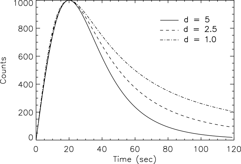
Figure 3: Examples of profiles of the power-law rise-model for three different power-law indices during the decay phase; $d=5$ (solid line), $d=2.5$ (dashed line), $d=1$ (dashed-dotted line).

This four parameter model fully describes a single pulsed GRB event with direct measurements of an observed light curve yielding the values for $F_{\rm m},t_{\rm m},r,d$. This then gives $\tau_{\rm m}$, which in its turn, gives the product $E_{\rm m}\cdot\Phi_{\rm 0}$. As $E_{\rm m}$ can be measured from the $E_{\rm pk}$ decay, $\Phi_{\rm 0}$ can be deduced. Example profiles with varying decay parameters for the power-law rise-model are shown in Figure 3.

It must be noted that in this scenario (rise+decay), the HIC power law index, $\eta^{\prime}$, will correspond to both the implicit power law behavior, $E^{\eta}$ as well as the explicit behavior, $t^{r}$. Here $\eta^{\prime}$ denotes the power law in the second description. The two descriptions coincide as $r$ tends to $0$ and as $E_{\rm pk,0}\rightarrow E_{\rm m}$ which gives

$$F=\frac{F_{\rm m}}{\left(1+\frac{t}{(d-1)\tau_{\rm m}}\right)^{d}}$$ (24)

and thus $T=\tau_{\rm m}$ by identification. Note that $t_{\rm m}$ tends to $0$ as $r$ approaches $0$. It is also readily seen that the asymptotic behaviors as $t$ approaches $\infty$ are the same.

2.1.2 Exponential Rise

It is reasonable that the rise phase is connected to some transient process, e.g., an initial decrease in optical depth, increase in the number of energized particles, or the merging (or crossing) of two shells. After this initial phase, the original decay behavior as described by equations (14) and (15) should emerge. We therefore try the following prescription

$$f(t)\propto 1-e^{-t/\tau_{\rm r}}$$ (25)

where the time constant $\tau_{\rm r}$ now represents the rise phase. This corresponds to $h(t)\propto g(t)^{\eta}$ as $t>>\tau_{\rm r}$. We therefore have

$$F=F_{\rm m}\left(\frac{E_{\rm pk}}{E_{\rm m}}\right)^{\eta}\frac{1-e^{-t/\tau_{\rm r}}}{1-e^{-t_{\rm m}/\tau_{\rm r}}}$$ (26)

which gives the differential equation

$$\dot{E_{\rm pk}}=-\frac{F_{\rm m}E_{\rm pk}^{\eta}(1-e^{-t/\tau_{\rm r}})}{\Phi_{\rm 0}E_{\rm m}^{\eta}(1-exp(-t_{\rm m}/\tau_{\rm r}))}$$ (27)

In the same manner as before we define the decay index $d$ by requiring $F(t)\rightarrow t^{-d}$ as $t\rightarrow\infty$. This gives $\eta=d/(d-1)$. Solving the differential equation (27) and combining with equation (26) we find

$$F(t)=\frac{A_{0}(1-e^{-t/\tau_{\rm r}})}{(1+(t+\tau_{\rm r}e^{-t/\tau_{\rm r}})/\tau_{\rm d})^{d}}$$ (28)

$$E_{\rm pk}(t)=\frac{A_{1}}{(1+(t+\tau_{\rm r}e^{-t/\tau_{\rm r}})/\tau_{\rm d})^{(d-1)}}$$ (29)

where $A_{0}$ and $A_{1}$ are analytical functions of $d,\tau_{\rm d},\tau_{\rm r},\Phi_{\rm 0},F_{\rm m},E_{\rm m}$ and $t_{\rm m}$. There is no analytical expression for the peak time $t_{\rm m}$, but it can be solved for numerically if the other parameters are known. Equation (28) describes the pulse by four parameters: $A_{0},\tau_{\rm r},\tau_{\rm d},$ and $d$. This description coincides with the decay function (eqs. [14] and [15]) when $\tau_{\rm r}\rightarrow 0$ or $t\rightarrow\infty$ with $\tau_{\rm d}\rightarrow(d-1)T$ (and $E_{\rm m},F_{\rm m}\rightarrow E_{\rm pk,0},F_{\rm 0}$). Note that in this description there are two explicit time constants $\tau_{\rm r}$ and $\tau_{\rm d}$, while in equation (22) the decay constant is an expression of $r$ and $t_{\rm m}$. For a sharp rise phase the explicit time dependence will disappear. This is, however, not the case for equation (22).

3 Data Analysis

For the purposes of this study, we utilize 64ms count data provided by the BATSE instrument onboard the CGRO spacecraft. These data were gathered by BATSE’s Large Area Detectors (LADs) which provide discriminator rates with 64 ms resolution from 2.048 s before the burst to several minutes after the trigger (Fishman et al., 1994). The discriminator rates are gathered in four broad energy channels covering approximately 25-50, 50-100, 100-300, and 300 to about 1800 keV allowing for excellent count statistics since the photons are collected over a wide energy band. For our analysis, we combine the data from all four channels in order to study the ”bolometric” light curve profile. We chose to study the count flux light curves rather then directly using the energy flux because of the spectral fitting that is trespassory to obtain energy flux measurements. Although BATSE’s spectroscopic detectors (SDs) can gather enough data to produce spectra on a 0.128 s timescale, the data usually has to be integrated to get an acceptable fit to a given spectra model. This reduces the resolution of the energy flux time history to a level that is unacceptable for a four or five parameter fit. Furthermore, Borgonovo & Ryde (2003) have shown that, empirically, there is a power-law relation between the count flux and the energy flux, with an index clustering around $1$, which supports the use of the count light-curves for our study of the pulse shapes. The background is, in general, fitted to a quadratic polynomial using 1.024 s resolution background data that are available from 10 minutes before the trigger to several minutes after the burst. The data along with the background fit coefficients were obtained from the CGRO Science Support Center (GROSSC) at Goddard Space Flight Center through its public archives.

We selected bursts from the entire BATSE catalog with the criteria that the peak flux be greater than 1.0 photons cm^-2 s^-1 on a 256 ms timescale. Of these, we selected bursts that exhibited clean, single-peaked events, or in the case of multi-peaked bursts, pulses that were well distinguished and separable from each other. We limited the bursts to events with durations longer than 2 s (full width half max - FWHM), primarily because this study focuses on the properties of long GRB events. There are strong indications that short bursts with $T_{90}<2.6$ s have different temporal behaviors compared to long bursts and that they may actually constitute a different class of GRBs (Norris, Scargle, & Bonnell, 2001). Therefore, in this study we are primarily interested in the shape and temporal properties of long GRB events. In the search we did not assume any functional description of the pulse profile, i.e. pulses that did not look like FREDs were also selected, in order to eliminate any preconceived idea of what the fundamental pulse shape should be. We note that we do not know what the clean, ”generic” pulse actually looks like, and some noise, or substructure, in the comoving light curve can be expected, for instance, if the surface brightness of the shell is non-homogeneous and/or if the density profile of the shell, through which the shock is traversing, has a complicated radial profile. Therefore, we adopt the following criteria. If a significant substructure on top of a smoothly fitted pulse is within a time interval of 1/4 the FWHM of the main pulse peak and it contains more than 15 $\%$ of the total flux in the main pulse, the pulse structure is rejected. If the substructure occurs in a time interval of more than twice the FWHM of the primary pulse, then the pulse is treated as an independent event and is fitted separately. We believe that this limits the possible contamination of the sample with pulses that are actually a composite of overlapping emission episodes. The final sample consisted of 76 pulses within 68 bursts. This sample differs from those examined in previous studies such as Norris et al. (1996) because they primarily represent separable pulses that exhibit long decay tails that can be followed to background. Therefore, no attempt was made to perform deconvolution fits of overlapping pulses, for the purpose of obtaining robust measurements of the asymptotic decay of each pulse, which is not possible for overlapping regions of activity. For more details on the sample selection, see F. Ryde $\&$ D. Kocevski (in prep.). These bursts are presented in Table 1, and are denoted by both their GRB names and BATSE trigger numbers. The pulses within multi-peaked bursts are distinguished by their $t_{max}$ value.

All of the background-subtracted light-curves were fitted with the power-law rise- (eq. 22) and the exponential rise- (eq. 28) functions via $\chi^{2}$ minimization. To aid in this, we developed a graphical IDL fitting routine which allowed the user to set the initial pulse attributes manually before allowing the fitting routine to converge on the best fit model. The convergence routine utilized the Marquardt technique to minimize the difference between the model and the time profile by adjusting the model parameters and tracking the resulting effects on the $\chi^{2}$. In the case of the power-law rise-function, the free parameters were: peak flux $f_{max}$, position of peak flux $t_{max}$, the rise index $r$, and the decay index $d$. Most of the GRBs had significant emission prior to the BATSE trigger time, so we introduced a fifth parameter $t_{0}$ which measures the offset between the start of the pulse and the trigger time. The initial value of $t_{0}$ was typically set to where the light curve would rise above 10$\%$ of the background, helping to eliminate the ambiguity associated with the start of the pulse. In the case of the exponential rise-function, the free parameters were: pulse amplitude $A_{0}$, rise time constant $\tau_{r}$, decay time constant $\tau_{d}$, the asymptotic decay power law index d, and the trigger offset $t_{0}$.

4 Results

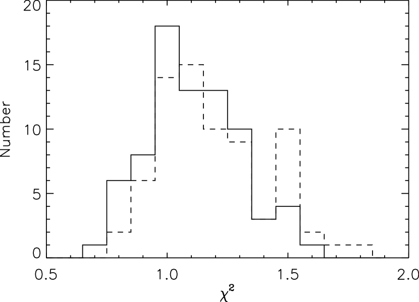
Figure 5: $\chi^{2}$ distributions for the power-law rise-model (solid line) and exponential rise-model (dashed line). A simple power-law representing the rise-phase provides an overall better fit to the data sample.

Presented in Figure 4 are four type-fits to the power-law rise-function (eq. 22). These pulses represent a good example of the clean separable FRED pulses chosen for this analysis and the degree of acceptability of $\chi^{2}$ for our fits. Overall the power-law rise-function appears to give a better fit to most of the pulses compared to the exponential rise-function (eq. 28). This can be seen in the spread of the respective $\chi^{2}$ distribution for our entire sample shown in Figure 5, with the power-law rise-model giving a mean $\chi^{2}$ of 1.16 with a standard deviation of 0.19. This is most likely due to the fact that the power-law function allowed for the modelling of both concave and convex rise profiles, whereas the nature of the exponential function is limited to modelling concave shapes. This is a major constraint for the latter model since many GRB pulses that are arguably single emission episodes are seen to have concave rise profiles, at least in the initial stage.

The narrow distribution of $\chi^{2}$ values also indicates that a power law is sufficient to model the decay portion of the pulse light curve. According to Fenimore et al. (1996), this would not be the case if evolution of the low energy spectral index $\alpha$ greatly affected the resulting light curve. As discussed in $\S 1$, they show that the decay phase should scale roughly as the power of the low energy spectral index $T^{-\alpha-1}$. If $\alpha$ exhibited a large range of evolution during the decay phase, then a single power law would no longer be adequate to model the temporal behavior of the light curve. The $\chi^{2}$ distributions support the assumption that the evolution of the low energy spectral index does not significantly alter our results.

4.1 Rise and Decay Timescales

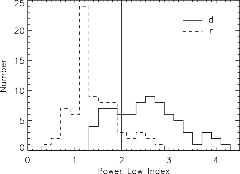
Figure 6: Distribution of the rise (dashed line) and decay (solid line) power-law indices for the power-law rise-model. The thick solid line represents the expected decay value if the pulse profile were produced purely by curvature effects.

The primary pulse attributes that can be derived from fitting the time profiles are related to the pulse rise and decay rates. In the case of the power-law rise-function, these consist of the asymptotic rise and decay power-law indices $r$ and $d$ described in $\S$2.3. The resulting $r$ and $d$ parameter distributions for our entire sample are shown in Figure 6. The rise index appears to be the tighter of the two, with a mean value of $\langle r\rangle=1.49\pm 0.25$ and a standard deviation of 0.63. The distribution of the decay index is somewhat broader with a mean value of $\langle d\rangle=2.39\pm 0.12$ with a standard deviation of 0.76. The exponential-rise function has no corresponding rise index, but rather the rise timescale is associated with the time constant $\tau_{r}$ in equation (28). The fit results show that the rise timescale covers a very broad range of values with a median value of $\langle\tau_{\rm r}\rangle=2.40\pm 0.10$ and a standard deviation of 2.50. The asymptotic decay index is similar to that found with the power law rise model except that it has a much broader distribution with a median value of $\langle d\rangle=2.75\pm 0.12$ with a standard deviation of 1.50.

4.2 Pulse Asymmetry

A measure of the average pulse time-asymmetry can be easily constructed using the fit parameters obtained from both models. Several authors have studied burst asymmetry properties in the past (Norris et al., 1996; Fenimore et al., 1996) - and found interesting correlations between the pulse asymmetries and other temporal properties. Norris et al. (1996) measured asymmetry values for some 400 fitted pulses and reported a general trend that narrower pulses tend to be more symmetric and have harder spectra. This is often referred to as the GRB pulse paradigm. Here we define the asymmetry as the fraction of the FWHM belonging to the rise phase of the pulse to the fraction belonging to the decay phase (see Figure 7 for an illustration). This description is independent of the model parameters used to fit the pulses and hence allows the asymmetry to be measured for both of the functions utilized in this analysis in a comparative manner. The resulting asymmetry distribution for the power-law rise-model is remarkably tight with a median value of 0.47 $\pm$ 0.08 and a standard deviation of 0.09. The exponential rise model provides similar results yielding a median value of 0.45 $\pm$ 0.07 and a standard deviation of 0.07.

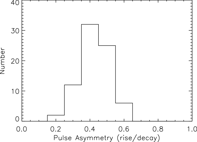
Figure 8: Pulse asymmetry distribution for the power law rise model as measured by taking the ratio of the rise to decay times, see section §4.2 for a complete definition. The distribution peaks at 0.47 $\pm$ 0.08.

Alternatively, the asymmetry can be defined using the $T_{90}$ of the pulse instead of the FWHM. The rise phase would then be defined as the interval from when where 5$\%$ of the pulse counts are accumulated till the time of peak flux as measured by the model parameter $t_{max}$. Similarly, the decay phase is simply the time between the peak flux till when 95$\%$ of the pulse counts are collected. Note that here we are using $T_{90}$ for the individual $pulses$, not the entire burst which is the common practice. Although this description is straightforward, it is somewhat more problematic when dealing with multi-pulsed bursts because subsequent pulses will routinely begin before the signal from the first pulse falls to within 5$\%$ of the background. It is presumed that the decay phase of the pulse is hidden under the rise phase of the following pulse, therefore in these cases the decay time is only a lower limit to the true length of the decay phase of the pulse. This occurred in 10$\%$ of the pulses observed, so the effect on the overall distribution should be minimal. The resulting median asymmetry values using the $T_{90}$ definition for both the power law and exponential models are 0.30 $\pm$ 0.04 and 0.21 $\pm$ 0.03 respectively. The resulting asymmetry distributions for the power-law rise-function for the FWHM definition is plotted in Figure 8.

Surprisingly, we find no evidence of a connection between the pulse asymmetry and the pulse duration ($T_{90}$) for the individual FRED pulses. Likewise, we find no significant correlations between the pulse asymmetry and the pulse width (FWHM). The lack of any significant correlation can be seen in Figure 9 and measured quantitatively by the use of the Spearman rank-order statistic which provides a robust and convenient means of evaluating the statistical significance of a given correlation. A Spearman rank order analysis on the data shown in Figure 9 yields a correlation coefficient of $R=0.057$, where $R=1$ represents a 1:1 correspondence. Both of these conclusions are contrary to the pulse paradigm referred to earlier and the disagreement is most likely due to the difference in samples used in the two studies. The Norris et al. (1996) study examined complex overlapping bursts for a majority of their data sample, while the majority of our sample consist of single-peaked FRED bursts. This leads to the conclusion that most of the simple FRED pulses that were examined in our sample are extremely self-similar, independent of their duration and amplitude.

4.3 Correlations

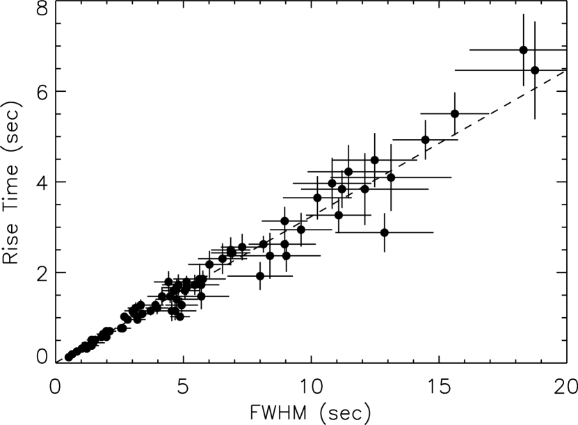
Figure 10: Rise time vs. the FWHM as measured by the model with a power-law rise. The linear correlation is a manifestation of the tight asymmetry distribution. The correlation coefficient yields a value of $R=0.981$.

We now examine several correlations between temporal properties measured from the pulse profiles such as the FWHM, rise and decay times and fluence values. First, Figure 10 shows the pulse rise time versus the pulse width, as measured by the FWHM, for our entire sample. The resulting linear correlation has a slope of 0.323 $\pm$ 0.01 with an associated Spearman rank order correlation coefficient of $R=0.981$ and is a direct consequence of the tight asymmetry distribution discussed above. This same effect is also observed between the time constant $\tau_{r}$ derived from the exponential rise model and the pulse width. Here again, the rise time constant, which is an alternative way of measuring the characteristic rise timescale, is linearly correlated to the FWHM. Note that the FWHM values plotted in Figure 10 are not normalized to any timescale such as the pulse duration, reasserting that the rise time is a constant fraction of the overall pulse width independent of the duration of the pulse.

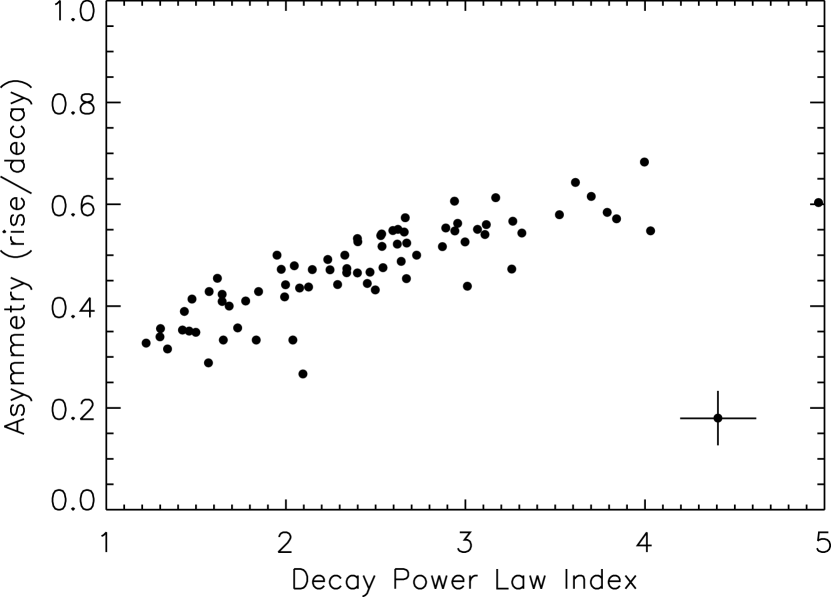
Figure 12: Asymmetry plotted vs. the decay power-law index. Pulses with higher decay indices appeared slightly less symmetric, with a correlation strength of $R=0.831$. The average error is illustrated in the bottom right corner.

Another correlation born from the data is the relationship between the normalized rise time and the decay power-law index, which is shown in Figure 11 and has a correlation coefficient of $R=0.799$. Here the rise time is normalized to the FWHM of the pulse, so the longer the rise time is, relative to the FWHM, the steeper the resulting power-law decay of the pulse envelope becomes. This is very interesting since the rise time is thought to be proportional to the dynamic or shell-crossing time of the pulse and is generally believed to be independent of the subsequent fall of the FRED profile. A similar effect can be seen in Figure 12 where the pulse asymmetry data are plotted versus the asymptotic decay power-law index. The degree of asymmetry is seen to be proportional ($R=0.831$) to the decay index in such a way that pulses with steep decay profiles (large $d$) have a larger rise-to-decay ratio. The latter correlation is to be expected since, as $d$ tends to 0, the decay time approaches $\infty$ and hence the asymmetry tends to 0. A similar correlation is not seen with the rise power-law index.

5 Discussion

The fit results presented above indicate that the analytic functions derived in §3 are very successful in describing the overall profile of individual GRB pulses. These descriptions differ from those used in previous modelling surveys as they are motivated by physical first principles within the general fireball model with the requirement that the previously observed empirical relations for the spectral evolution must hold. These descriptions also build on the original Ryde & Svensson (2002) analysis by including a description of the rise phase of the pulse. Of the two assumed rise profiles presented in §2, a simple, power-law rise seems to better describe the majority of the FRED pulses examined. This is one of the simplest assumptions that can be made regarding the dynamic (or shell crossing) phase of a GRB pulse and may point to the explicit time-dependance of the parameters internal to the shock such as Thompson depth or the magnetic field. Hence, the measured pulse parameters have the potential to be used to diagnose pulse characteristics, such as bulk Lorentz factors, $\Gamma$, shell radii, and thickness.

The decay power-law index appears to cover a wide range of values with a median centered around 2.39 $\pm$ 0.12, which is 3.25 $\sigma$ steeper than the analytically derived value of $d=2$ for pulse profiles created principally by relativistic effects due to spherical symmetric shells. Overall, 30 of the 77 pulses that we analyzed had decay indices that were consistent (within 1$\sigma$) with the predicted $d=2$ value, constituting 39$\%$ of our sample. We note that the distribution of HIC indices, which were shown in $\S 2$ to be directly related to the decay index, found by Borgonovo & Ryde (2001) also has a broad distribution, with several cases differing substantially from $\eta=2$. There are several mechanisms that can cause the decay envelope to deviate from the predicted spherical scenario, but the most obvious would be the breaking of local spherical symmetry. Both prolate and oblate shell geometries as seen by the observer would create light curves with resulting power-law indices that differ from the spherical case. In $\S 1$ we derived the shape that the light curve is expected to take if the pulse profile were created purely by a spherical shell. In the case of an elliptical geometry, the time delay between the arrival of off axis photons will be given by $\Delta t=(R_{0}-R\mu)/c$, where $R_{0}$ is the radius of the shell at $\theta=0$. The radius $R$ of the shell is no longer independent of the angle $\theta$, and is given by

$$R=a\sqrt{\frac{1-e^{2}}{1-e^{2}\mu^{2}}}$$ (30)

where e is the eccentricity of the shell, a is the semi-major axis, and $\mu=cos(\theta)$. Substituting this back into $\Delta t$, we find that

$$\Delta t=a-a\sqrt{\frac{1-e^{2}}{1-e^{2}\mu^{2}}\mu}$$ (31)

Solving for $\mu$ and substituting into the Doppler boost expression (equation 3) gives the Doppler profile (Doppler boost as a function of time) for elliptical shells

$${\cal D}(\Gamma,t)=\frac{1}{\Gamma(1-\frac{\beta(-t+a)}{\sqrt{e^{2}t^{2}-2e^{2}ta-a^{2}}})}$$ (32)

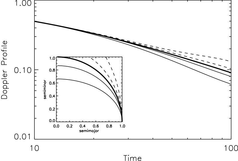
Figure 13: Resulting Doppler profiles for various shell geometries (shown in the inset). The prolate shells (dashed) yield a Doppler profile that is steeper than the spherical case (thick solid), whereas the emission from oblate geometries (dashed) will be observed to decay more slowly.

Following from the discussion in $\S 1$, the resulting evolution of the spectral break-energy and light curve of the energy-flux should follow $E_{\rm pk}(t)=E^{\prime}_{\rm pk}{\cal D}$ and $F_{bol}(t)=F_{0}{\cal D}^{2}$, so the profile of the varying Doppler boost should directly give rise to the time dependence of the $E_{pk}$ evolution and the pulse light curve. The Doppler profile, expressed in equation 32, is shown for several different prolate and oblate shock fronts in Figure 13, with the corresponding shell geometry plotted as an inset. It shows that the prolate shells (solid lines) have steeper Doppler profiles resulting in asymptotic power law slopes which are greater than the spherical case (thick solid line) whereas the opposite is true for the oblate geometries (dashed lines). The extreme limit of the oblate scenario is such that the shell becomes a parallel slab, in which case for an unresolved source the Doppler profile approaches zero and any pulse evolution is directly due to the shell’s intrinsic emission profile. Because of this effect, the observed range of power-law decay indices may be explained by a simple distribution of shell geometries, where the median decay index of 2.39 $\pm$ 0.12 would indicate that, in the context of relativistic curvature, the majority of the analyzed pulses were produced by shells with a degree of curvature greater than that exhibited by a spherical shell. Such conditions are not unreasonable in the context of the fireball model and a simple angular dependance of the bulk Lorentz factor can easily produce an elliptical shock front that evolves as the shock propagates. The evolution of the shock geometry, from oblate at early times to prolate at later times, and a variation in the time at which the shell ”ignites” during this evolution, could account for the distribution of decay indices.

Fenimore et al. (1996) and Fenimore & Sumner (1997) provide several other arguments in support of the breaking of local spherical symmetry, the most prominent being that the pulse photon light curves appear to evolve uncoupled to the GRB spectra. They find that the GRB spectra also evolve faster than the predicted rate of evolution due to the simple boost factor that is expected from a spherically symmetric shell. According to the investigation performed by Ryde & Petrosian (2002), this result is consistent with our findings that the average light curve profile also decays faster than predicted. In the context of their model, a range of relative sizes between the comoving and the curvature timescales defined in $\S 1$ can result in a variety of pulse shapes. Light curves that exhibit a substantially different shape than that predicted by spherical curvature are attributed to a scenario where the comoving timescale dominates within a burst that already has an intrinsically fast decay rate ($d>2$) of the comoving light curve. This, according to their model, must also be manifested in the spectral evolution in a corresponding manner. Therefore, an analysis of the spectral evolution rates and $\alpha$ values of the pulses that vary the furthest from the predicted scenario of $d=2$ may test how much these values affect the resulting light curve profiles. This research is currently being pursued (F. Ryde,& D. Kocevski in prep).

The asymmetry results are rather surprising and the reason for the tight asymmetry distribution among such a variety of GRB pulses is not immediately clear. It would indicate that the dynamical and angular timescales are not fully independent and that the observed rate at which the shell becomes active is dependant on the decay timescale and hence the curvature of the shell. A situation can be envisioned where a short comoving rise profile is delayed and boosted to the same degree as the shell’s intrinsic cooling profile. If both of these timescales are extremely short as compared to the angular spreading timescale, then a relationship can be produced between the observed rise and decay profile. This effect could produce a narrow asymmetry distribution and would also predict a correlation between the rise timescale and decay power-law indices, which is indeed observed in our sample. Ryde & Petrosian (2002) have discussed extensively the effect of varying intrinsic emission profiles and angular spreading timescales on the resulting light curve that is observed. They find that the resulting pulse asymmetry relies heavily on the convolution of the intrinsic emission profile and the angular spreading timescale. Therefore, future modelling of pulse timescales and shell geometries, with the constraint that they produce the observed asymmetry distribution, may yield clues to the intrinsic profile of the emission episode.

Figure 1: (a) Background subtracted (64ms resolution) count light-curve (energy range: KeV) for GRB 930612 (BATSE trigger 2387), a quintessential FRED pulse. (b) Similar light-curve for GRB 960113 (trigger 4350) which exhibits three separable FRED pulses.

Figure 4: Examples of fits to the power-law rise-model for GRB 911016b (trigger 907), GRB 000323 (8049), GRB 910721b (563), and GRB 980718a (6930). See Table 2 for the associated fit parameters.

Figure 7: Rise and decay times used to calculate the pulse asymmetry are defined as the fraction of the FWHM before and after the time of peak emission, ${t_{\rm max}}$. This example has a rise index of $r=1$ and a decay index of $d=2$.

Figure 9: Pulse asymmetry vs. the pulse duration ($T_{90}$) showing no correlation between the length of the pulse to the ratio of its rise and decay timescales. The correlation coefficient is $R=0.057$.

Figure 11: Decay power-law index plotted vs. the normalized rise time. The time to peak is correlated to the hardness of the decay profile with a correlation coefficient of $R=0.799$. This again is an effect of the narrow asymmetry distribution exhibited by the pulses. The average error is illustrated in the bottom right corner.

Table 1: Burst Sample with Select Model Parameters.

Burst	Trigger	$T_{max}$	Peak Intensity	$T_{90}$	Power Law Index		Model Fits
Name	Number	(s)	(photons s-1 cm-2)	(s)	Rise	Decay	$\chi_{p}^{2}$	$\chi_{e}^{2}$
910721	563	1.65	2.13 $\pm$ 0.29	24.8 $\pm$ 3.97	0.77 $\pm$ 0.15	1.34 $\pm$ 0.07	1.34	1.34
911016	907	1.47	3.74 $\pm$ 0.34	19.7 $\pm$ 2.56	0.85 $\pm$ 0.11	1.46 $\pm$ 0.05	1.29	1.29
911022	914	0.55	2.64 $\pm$ 0.33	6.27 $\pm$ 0.76	1.81 $\pm$ 0.10	2.33 $\pm$ 0.14	0.86	0.96
911031	973	2.87	5.71 $\pm$ 0.41	17.9 $\pm$ 0.99	1.23 $\pm$ 0.08	3.07 $\pm$ 0.10	1.34	1.35
911031	973	23.9	3.17 $\pm$ 0.40	17.9 $\pm$ 2.03	1.21 $\pm$ 0.23	2.15 $\pm$ 0.09	1.27	1.33
911104	999	3.94	12.4 $\pm$ 0.65	1.98 $\pm$ 0.20	2.40 $\pm$ 0.33	2.73 $\pm$ 0.07	1.24	3.05
911209	1157	4.83	12.2 $\pm$ 0.55	8.58 $\pm$ 1.07	1.60 $\pm$ 0.58	1.62 $\pm$ 0.10	1.30	1.58
920216	1406	3.14	2.10 $\pm$ 0.27	25.1 $\pm$ 3.18	0.95 $\pm$ 0.07	2.29 $\pm$ 0.11	1.06	1.07
920307	1467	4.32	2.59 $\pm$ 0.27	18.3 $\pm$ 2.05	2.53 $\pm$ 0.08	2.62 $\pm$ 0.08	1.01	1.06
920801	1733	3.30	3.20 $\pm$ 0.32	17.3 $\pm$ 1.73	1.97 $\pm$ 0.08	2.05 $\pm$ 0.06	1.17	1.29
920830	1883	1.26	5.36 $\pm$ 0.37	8.19 $\pm$ 0.51	1.48 $\pm$ 0.04	2.60 $\pm$ 0.08	1.06	1.07
920925	1956	2.81	2.80 $\pm$ 0.28	10.7 $\pm$ 1.04	1.31 $\pm$ 0.38	3.31 $\pm$ 0.22	1.47	1.50
921015	1989	116	2.96 $\pm$ 0.31	18.3 $\pm$ 1.83	2.00 $\pm$ 0.18	2.40 $\pm$ 0.06	1.35	1.66
921207	2083	8.59	46.6 $\pm$ 0.92	4.00 $\pm$ 0.20	2.12 $\pm$ 0.05	1.85 $\pm$ 0.02	1.25	1.71
921218	2102	1.88	1.79 $\pm$ 0.26	10.9 $\pm$ 1.51	1.90 $\pm$ 1.03	2.94 $\pm$ 0.29	0.89	0.95
930120	2138	1.50	7.08 $\pm$ 0.39	9.73 $\pm$ 1.27	2.00 $\pm$ 0.06	4.00 $\pm$ 0.20	1.28	1.15
930120	2138	48.9	35.6 $\pm$ 0.59	9.73 $\pm$ 1.77	1.46 $\pm$ 0.47	2.23 $\pm$ 0.29	0.96	1.00
930120	2138	86.1	9.81 $\pm$ 0.10	15.0 $\pm$ 1.18	0.42 $\pm$ 0.06	2.10 $\pm$ 0.11	1.29	1.35
930214	2193	10.9	1.78 $\pm$ 0.26	70.3 $\pm$ 10.3	0.80 $\pm$ 0.01	2.50 $\pm$ 0.04	1.04	1.02
930612	2387	6.57	4.11 $\pm$ 0.33	32.8 $\pm$ 2.91	1.20 $\pm$ 0.04	2.87 $\pm$ 0.06	1.07	1.17
930807	2484	1.87	1.75 $\pm$ 0.27	13.5 $\pm$ 1.87	1.26 $\pm$ 0.29	3.26 $\pm$ 0.43	1.10	1.17
930909	2519	63.5	1.68 $\pm$ 0.28	15.0 $\pm$ 3.21	1.69 $\pm$ 0.16	1.43 $\pm$ 0.12	1.13	1.21
930914	2530	114	2.03 $\pm$ 0.27	25.3 $\pm$ 3.28	1.12 $\pm$ 0.05	2.34 $\pm$ 0.12	1.13	1.14
931127	2662	1.10	1.82 $\pm$ 0.29	14.9 $\pm$ 2.94	1.20 $\pm$ 0.05	1.30 $\pm$ 0.03	1.07	1.04
931128	2665	1.34	2.10 $\pm$ 0.31	12.8 $\pm$ 2.25	1.74 $\pm$ 0.43	1.65 $\pm$ 0.10	1.00	1.16
931221	2700	53.8	4.17 $\pm$ 0.35	13.0 $\pm$ 1.13	0.75 $\pm$ 0.09	3.01 $\pm$ 0.18	1.33	1.52
940313	2880	0.4	3.20 $\pm$ 0.29	4.16 $\pm$ 0.54	1.32 $\pm$ 0.27	2.13 $\pm$ 0.15	1.51	1.61
940410	2919	0.30	6.11 $\pm$ 0.39	10.6 $\pm$ 0.80	1.55 $\pm$ 0.14	1.97 $\pm$ 0.04	1.28	1.55
940529	3003	9.56	3.04 $\pm$ 0.32	28.8 $\pm$ 3.13	1.51 $\pm$ 0.04	2.62 $\pm$ 0.08	1.11	1.21
940830	3143	0.63	2.69 $\pm$ 0.29	5.5 $\pm$ 0.76	1.84 $\pm$ 0.68	2.40 $\pm$ 0.14	1.04	1.16
940904	3155	0.66	1.92 $\pm$ 0.26	3.39 $\pm$ 0.46	1.24 $\pm$ 0.21	3.84 $\pm$ 0.60	0.88	1.01
941023	3256	1.25	1.89 $\pm$ 0.22	14.0 $\pm$ 2.68	0.80 $\pm$ 0.02	1.50 $\pm$ 0.04	1.28	1.16
941026	3257	3.27	3.21 $\pm$ 0.27	36.8 $\pm$ 5.49	0.52 $\pm$ 0.04	1.57 $\pm$ 0.07	1.02	1.08
941026	3259	4.65	2.28 $\pm$ 0.23	25.0 $\pm$ 3.28	1.55 $\pm$ 0.17	2.89 $\pm$ 0.16	0.96	1.15
941121	3290	2.91	10.9 $\pm$ 0.36	1.98 $\pm$ 0.47	1.47 $\pm$ 0.25	2.04 $\pm$ 0.09	0.92	1.52
950211	3415	0.25	10.3 $\pm$ 0.40	6.91 $\pm$ 1.77	2.76 $\pm$ 2.14	1.68 $\pm$ 0.15	0.99	1.22
950211	3415	11.5	2.36 $\pm$ 0.11	3.78 $\pm$ 0.34	1.26 $\pm$ 0.14	2.47 $\pm$ 0.17	1.48	1.36
950624	3648	2.65	5.91 $\pm$ 0.31	22.0 $\pm$ 3.97	0.84 $\pm$ 0.44	2.67 $\pm$ 0.60	0.82	0.82
950624	3648	24.1	36.6 $\pm$ 1.22	17.0 $\pm$ 3.51	1.10 $\pm$ 0.04	2.40 $\pm$ 0.14	1.03	0.97
950624	3648	40.9	1243 $\pm$ 3.71	11.7 $\pm$ 1.16	2.54 $\pm$ 0.07	1.57 $\pm$ 0.03	1.45	1.19
950818	3765	66.1	25.9 $\pm$ 0.54	8.83 $\pm$ 0.98	2.42 $\pm$ 0.07	1.84 $\pm$ 0.02	1.50	1.43
951016	3870	0.43	14.1 $\pm$ 0.46	5.76 $\pm$ 0.52	1.38 $\pm$ 0.09	1.42 $\pm$ 0.02	1.52	1.78
951019	3875	0.21	3.02 $\pm$ 0.23	4.03 $\pm$ 0.42	0.96 $\pm$ 0.11	1.73 $\pm$ 0.13	1.57	1.51
951030	3886	0.20	2.27 $\pm$ 0.21	2.82 $\pm$ 0.65	1.27 $\pm$ 0.12	2.45 $\pm$ 0.27	1.00	1.55
951102	3892	0.61	1.86 $\pm$ 0.20	5.31 $\pm$ 0.51	1.26 $\pm$ 0.24	2.67 $\pm$ 0.29	0.97	1.03
951213	3954	0.70	8.45 $\pm$ 0.39	10.3 $\pm$ 0.70	4.31 $\pm$ 3.52	2.54 $\pm$ 0.50	1.06	1.52
951228	4157	7.67	2.32 $\pm$ 0.24	17.7 $\pm$ 2.16	1.92 $\pm$ 0.09	2.53 $\pm$ 0.12	1.21	1.36
960113	4350	0.51	3.52 $\pm$ 0.25	6.66 $\pm$ 0.83	2.41 $\pm$ 0.16	1.95 $\pm$ 0.07	1.29	1.86
960113	4350	14.3	1.65 $\pm$ 0.27	6.66 $\pm$ 0.75	1.00 $\pm$ 0.02	2.00 $\pm$ 0.03	1.39	1.22
960113	4350	34.1	8.71 $\pm$ 0.45	6.66 $\pm$ 0.98	1.70 $\pm$ 0.34	2.66 $\pm$ 0.23	1.30	1.47
960114	4368	2.45	58.6 $\pm$ 0.83	10.0 $\pm$ 0.75	2.87 $\pm$ 0.68	2.53 $\pm$ 0.07	1.26	2.01
960530	5478	1.98	3.10 $\pm$ 0.24	14.3 $\pm$ 1.43	0.98 $\pm$ 0.08	2.54 $\pm$ 0.17	0.97	0.98
960530	5478	261	7.69 $\pm$ 1.70	37.2 $\pm$ 6.22	1.20 $\pm$ 0.02	3.00 $\pm$ 0.08	1.12	1.16
960613	5495	0.23	2.39 $\pm$ 0.23	5.44 $\pm$ 1.66	0.63 $\pm$ 0.34	1.65 $\pm$ 0.16	1.16	1.14
960624	5517	0.83	2.06 $\pm$ 0.23	7.42 $\pm$ 0.79	1.72 $\pm$ 0.11	3.61 $\pm$ 0.37	1.04	1.05
960628	5523	1.03	3.73 $\pm$ 0.28	6.98 $\pm$ 0.71	1.92 $\pm$ 0.07	3.17 $\pm$ 0.15	1.19	1.34
960715	5541	1.32	1.84 $\pm$ 0.23	12.6 $\pm$ 1.68	1.51 $\pm$ 0.47	2.96 $\pm$ 0.39	1.13	1.16
960912	5601	7.55	4.94 $\pm$ 0.29	9.00 $\pm$ 0.74	1.30 $\pm$ 0.26	2.64 $\pm$ 0.16	1.29	1.38
970405	6159	3.20	2.16 $\pm$ 0.25	12.0 $\pm$ 1.79	1.82 $\pm$ 0.13	1.30 $\pm$ 0.11	1.18	1.28
970815	6335	98.3	4.29 $\pm$ 0.29	21.3 $\pm$ 3.02	1.29 $\pm$ 0.08	3.52 $\pm$ 0.40	1.10	1.17
970925	6397	3.30	6.02 $\pm$ 0.30	20.4 $\pm$ 1.44	1.25 $\pm$ 0.07	2.25 $\pm$ 0.05	1.61	1.53
971127	6504	3.12	2.79 $\pm$ 0.24	22.1 $\pm$ 3.00	1.18 $\pm$ 0.12	1.78 $\pm$ 0.08	1.00	1.09
980301	6621	32.5	6.85 $\pm$ 0.34	7.36 $\pm$ 0.47	1.51 $\pm$ 0.05	1.65 $\pm$ 0.03	1.21	1.59
980302	6625	5.12	2.04 $\pm$ 0.26	31.4 $\pm$ 4.19	1.32 $\pm$ 0.05	3.12 $\pm$ 0.19	1.04	1.16
980401	6672	6.85	5.60 $\pm$ 0.29	3.80 $\pm$ 0.41	1.17 $\pm$ 0.07	2.34 $\pm$ 0.17	0.78	0.84
980718	6930	31.7	5.76 $\pm$ 0.36	6.34 $\pm$ 0.30	1.51 $\pm$ 0.04	3.70 $\pm$ 0.16	1.15	1.10
990102	7293	3.53	3.06 $\pm$ 0.23	25.2 $\pm$ 2.92	0.96 $\pm$ 0.07	1.99 $\pm$ 0.07	1.20	1.20
990102	7295	2.14	3.50 $\pm$ 0.35	8.50 $\pm$ 1.05	1.20 $\pm$ 0.42	2.08 $\pm$ 0.35	0.97	0.98
990316	7475	8.54	3.87 $\pm$ 0.29	34.4 $\pm$ 2.96	0.99 $\pm$ 0.07	4.03 $\pm$ 0.19	1.12	1.05
990505	7548	3.7	3.14 $\pm$ 0.25	10.6 $\pm$ 1.02	1.92 $\pm$ 0.46	2.94 $\pm$ 0.17	0.82	1.04
990528	7588	2.76	2.32 $\pm$ 0.24	15.5 $\pm$ 1.77	1.15 $\pm$ 0.13	3.11 $\pm$ 0.25	0.83	0.92
990707	7638	1.12	1.92 $\pm$ 0.22	15.0 $\pm$ 2.68	1.27 $\pm$ 0.30	1.22 $\pm$ 0.06	1.30	1.33
990712	7648	4.45	1.78 $\pm$ 0.21	24.7 $\pm$ 3.45	1.22 $\pm$ 0.13	3.79 $\pm$ 0.41	1.05	1.17
990816	7711	1.86	3.97 $\pm$ 0.26	13.2 $\pm$ 1.32	0.85 $\pm$ 0.04	3.26 $\pm$ 0.24	1.34	1.48
323	8049	30.5	1.77 $\pm$ 0.19	36.6 $\pm$ 4.23	1.13 $\pm$ 0.04	4.97 $\pm$ 0.42	1.04	1.24
519	8111	4.98	4.33 $\pm$ 0.28	13.8 $\pm$ 1.68	1.69 $\pm$ 0.03	1.48 $\pm$ 0.02	1.36	1.27

References

- Band et al. (1993) Band, D., et al. 1993, ApJ, 413, 281
- Borgonovo & Ryde (2001) Borgonovo, L., & Ryde, F. 2001, ApJ, 548, 770
- Borgonovo & Ryde (2003) Borgonovo, L., & Ryde, F. 2003, in proc. ”Gamma-ray bursts in the afterglow era”, 3rd workshop, Rome 17-20 Sept. 2002, in press
- Cheng et al. (1995) Cheng, L. X., Ma, Y. Q., Cheng, K. S., Lu, T., Zhou, Y. Y., 1995, AA, 300, 746
- Crider et al. (1999) Crider, A., Liang, E. P., Preece, R. D., Briggs, M. S., Pendleton, G. N., Paciesas, W. S., Band, D. L. , & Matteson, J. L. 1999, ApJ, 519, 206
- Eichler & Levinson (2000) Eichler & Levinson 2000, ApJ 529, 146
- Fenimore et al. (1996) Fenimore, E. E., Madras, C. D., & Nayakshin, S. 1996, ApJ 473, 998
- Fenimore & Sumner (1997) Fenimore, E., & Sumner, M. C. 1997, All-Sky X-Ray Observations in the Next Decade, 167
- Frail et. al. (2001) Frail, D. A., et. al. 2001, ApJ, 562, L55
- Fishman et al. (1994) Fishman, G. J., et al. 1994, ApJS, 92, 229
- Golenetskii et al. (1983) Golenetskii, S. V., Mazets, E. P., Aptekar, R. L., & Ilyinskii, V. N. 1983, Nature, 306, 451
- Lee et al. (2000a) Lee A., Bloom, E. D., & Petrosian, V. 2000a, ApJS, 131, 1
- Lee et al. (2000b) Lee A., Bloom, E. D., & Petrosian, V. 2000b, ApJS, 131, 21
- Liang & Kargatis (1996) Liang, E. P., & Kargatis, V. E. 1996, Nature, 381, 495
- Liang (1997) Liang, E. P. 1997, ApJ, 491, L15
- Liang, Kocevski, Boettcher (2003) Liang, E., Kocevski, D., Boettcher, 2003 in ASP Conf. Ser., Gamma Ray Burst and Afterglow Astronomy 2001, ed. G. Ricker and R. Vanderspek., in press
- Lloyd & Petrosian (2000) Lloyd, N., & Petrosian, V. 2000, ApJ, 543, 722
- Kobayashi, Ryde, & MacFadyen (2001) Kobayashi, S., Ryde, F., & MacFadyen, A. 2001, ApJ, 577, 302
- Kocevski & Liang (2002b) Kocevski, D., & Liang, E. 2002, in the proceedings of ’Gamma-Ray Burst and Afterglow Astronomy 2001’
- Norris et al. (1996) Norris, J. P., Nemiroff, R. J., Bonnell, J. T., Scargle, J. D., Kouveliotou, C., Paciesas, W. S., Meegan, C.A., & Fishman, G. J. 1996, ApJ, 459, 393
- Norris, Scargle, & Bonnell (2001) Norris, J. P., Scargle, J. D., & Bonnell, J. T. 2001, in Gamma-Ray Bursts in the Afterglow Era, eds. E. Costa, F. Frontera, & J. Hjorth (Berlin Heidelberg: Springer), 40
- Nemiroff et. al. (1994) Nemiroff, R. J., Norris, J. P., Kouveliotou, C., Fishman, G. J., Meegan, C. A., Paciesas, W. S.
- Piran (1999) Piran 1999, Physics Reports, 314, 575
- Preece et al. (1998) Preece, R. D., Briggs, M. S., Mallozzi, R. S., Pendleton, G. N., Paciesas, W. S., Band, D. L., 1998, ApJ, 506, L23
- Preece et al. (2000) Preece, R. D., Briggs, M. S., Mallozzi, R. S., Pendleton, G. N., Paciesas, W. S., & Band, D. L., 2000, ApJS, 126, 19P
- Ryde (1999) Ryde, F. 1999, Astrophys. Lett. Commun., 39, 281
- Ryde, Borgonovo, & Svensson (2000) Ryde, F., Borgonovo, L., & Svensson, R. 2000, in AIP Conf. Proc. 526, Gamma-Ray Bursts, 5th Huntsville Symposium, ed. R. M. Kippen, R. S. Mallozzi, & G. J. Fishman (New York: AIP), 180
- Ryde, Kocevski, & Liang (2003) Ryde, F., Kocevski, D., & Liang, E. 2003 in ASP Conf. Ser., Gamma Ray Burst and Afterglow Astronomy 2001, ed. G. Ricker and R. Vanderspek., in press
- Ryde & Petrosian (2002) Ryde, F., & Petrosian, V. ApJ, 578, 290
- Ryde & Svensson (1999) Ryde, F., & Svensson, R. 1999, ApJ, 512, 693
- Ryde & Svensson (2000) Ryde, F., & Svensson, R. 2000, ApJ, 529, L13
- Ryde & Svensson (2002) Ryde, F., & Svensson, R. 2002, ApJ, 566, 210
- Rybicki & Lightman (1979) Rybicki, G. & Lightman, A. Radiative Processes in Astrophysics (Wiley, New York, 1979).
- Tavani (1996) Tavani, M. 1996, ApJ 466, 768
- Wu & Fenimore (1996) Wu, B., Fenimore, E. 1996, ApJ 466, 768