Absolute calibration and beam reconstruction of MITO (a ground-based instrument in the millimetric region).

Abstract

An efficient sky data reconstruction derives from a precise characterization of the observing instrument. Here we describe the reconstruction of performances of a single-pixel 4-band photometer installed at MITO (Millimeter and Infrared Testagrigia Observatory) focal plane. The strategy of differential sky observations at millimeter wavelengths, by scanning the field of view at constant elevation wobbling the subreflector, induces a good knowledge of beam profile and beam-throw amplitude, allowing efficient data recovery. The problems that arise estimating the detectors throughput by drift scanning on planets are shown. Atmospheric transmission, monitored by skydip technique, is considered for deriving final responsivities for the 4 channels using planets as primary calibrators.

G. Savini^a A. Orlando^a E.S. Battistelli^a M. De Petris^a L. Lamagna^a G. Luzzi^a E. Palladino^a

^a Dipartimento di Fisica, Universitá ”La Sapienza”, P.le A.Moro 2, I-00185 Roma,Italy

1 Introduction

At millimeter wavelengths ground based cosmological observations are mainly constrained by atmospheric transmission and its time dependent emission as huge noise source. The largely employed observational technique, among collectors of submm/mm radiation, is differential measurements and consequent synchronous demodulation, $i.e.$ lock-in amplifiers technique. At MITO, in order to reduce the bulk of atmospheric emission, sky differential observations are obtained by a wobbling sub-reflector in a Cassegrain 2.6-m telescope. Modulation in the sky is usually performed as a 3-field square-wave function as to remove linear gradients of atmosphere in every direction. In the data recovery exact beam-throw amplitude and beam-shape have to be recovered for successive data analysis. This can be obtained, as we will show, by simulating the effect of systematics on the time ordered data. Different methods for beam shape extraction are then explained, and differences between the effects on calibration on point-source and extended beam-size objects outlined. Revised responsivity values obtained with the considered Jupiter temperature models are reported in section 4. In the last section, geometrical consequences on galaxy-cluster SZ-effect measurements are analyzed.

2 Data acquisition system.

Ground based telescopes observing a specific object in the sky can operate mostly in two different ways. One is chasing the object while moving in the sky, and the other is drift-scanning. Microphonics and side-lobe peak-ups prevent the possibility of tracking the source by moving the telescope: all our observations have been carried out in the so-called drift-scan mode. That is, the telescope is fixed, pointing a sky region which will be crossed by the source due to the natural Earth’s rotation. Since we know approximately the shape of our source we may predict the time-shape of the signal and only its peak amplitude remains a free parameter. In the present focal plane 4-bands single pixel photometer (FotoMITO), the voltage-signals of the bolometric detectors are filtered by commercial lock-in amplifiers (SR850). The use of lock-in amplifiers will be upgraded with a software-based acquisition system, allowing a great variety of offline demodulation techniques, in the new detector array instrumentation, MAD (Lamagna et al. 2002).

2.1 Retrieval of exact modulation amplitude.

Modulation of the secondary mirror is controlled by an electro-mechanical system with shakers in a push-pull configuration (Mainella et al. 1996), its position is read by a Linear Variable Differential Transformer (LVDT). Original optical design should allow us to retrieve information on sky modulation, the amplitude of which can be trimmed remotely. The exact modulation amplitude is checked by drift-scanning objects that can be treated as point-sources in respect to beam-size (like a planet $\sim 10^{\prime\prime}\div 40^{\prime\prime}$ in respect to $\sim 15^{\prime}\div 17^{\prime}$ FWHM of f.o.v.). If we assume a sampling rate of 1 Hz, then by knowing the distance between the two minima of the drift-scan, by adjusting for drift-modulation angle and knowing the speed of the object by its celestial declination, we can measure with good approximation the beam-throw of our telescope. Assumptions are that the shape of the beam is the same during modulation (primary goal during mirror design) (De Petris et al. 1996). In particular, this assumption has been verified by comparing the beam shape obtained with different methods (see.3). Precision of this measurement can be mined by atmospheric fluctuations (greatest noise source) in the proximity of the minima of the drift-scans (when a culminating source is in the center of the modulated beam). A solution is to find a polynomial best-fit around each minimum to obtain a reasonable identification of relative minima. If acquisition was achieved without hardware or software lock-in procedures, setting aside noise problems, and with beam-throws considerably greater than the width of the beam at -30dB so to avoid contamination and averaging as we do on 3 modulation periods, we would reasonably have 3 distinct beam-shapes (for a culminating source) separated by a small baseline. As beam-throw decreases contamination sets in and the three shapes start to merge.

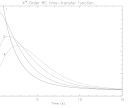
Figure 1: First to fourth order time impulse response function of the Lock-in low-pass integration circuit.

Moreover Lock-in techniques introduce time-integration due to their internal filter to extract the locked frequency with a steep cut. In our case (hardware and software) a $4^{th}$ order RC circuit filter has been employed (fig.1). Setting the time-constant of the lock-in determines the impulse-response that is applied to acquired data in the time domain. This introduces a progressive time-shift that becomes constant after a certain number ($10\div 20$) of time-constants. If base-lines (acquisition of atmospheric signal before and after the source enters the modulating beam) are sufficiently long, the shift sets in and no correction for time separation of minima is needed. If not, it would be necessary to ”de-convolve” the signal from the time-impulse, but this can be done only on the final averaged data points. To do so we sample the time-domain transfer function at the same rate of our final data (i.e. 1 per second) in a vector $K=\{k_{i}\}$. In this way the data set $D=\{d_{i}\}$ can be viewed as the result of the following operation on the true ”would-be” data $T=\{t_{i}\}$:

$$D=\frac{(K\circ T)}{A}\ \ \ \ \ \bigl{(}\mbox{ with }A=\sum_{i=0}^{n-1}k_{i}\bigr{)}$$ (1)

In this way if we make the non restrictive hypothesis that non-acquired data before the beginning of our drift (like an extended base-line) is zero, or in the case of a constant baseline with a non-zero signal, equal to that offset (we consider a zero baseline for calculations), we obtain the recursive process:

d_0 = t_0k_0/A ,

$$d_{1} = (t_{1}k_{0}+t_{0}k_{1})/A,$$

$$d_{i} = \sum_{j=0}^{i}(t_{i-j}k_{j})/A\ \ \ \mbox{for}\ i<n,$$

$$d_{i} = \sum_{j=0}^{n-1}(t_{i-j}k_{j})/A\ \ \ \mbox{for}\ i\geq n$$ (2)

that under the cited assumptions can be solved backwards in

t_0 = Ad_0/k_0 ,

$$t_{1} = (Ad_{1}-t_{0}k_{1})/k_{0},$$

$$t_{i} = \bigl{(}Ad_{i}-\sum_{j=1}^{i}(t_{i-j}k_{j})\bigr{)}/k_{0}\ \ \ \mbox{for}\ i<n,$$

$$t_{i} = \bigl{(}Ad_{i}-\sum_{j=1}^{n-1}(t_{i-j}k_{j})\bigr{)}/k_{0}\ \ \ \mbox{for}\ i\geq n$$ (3)

The obtained vector (fig.2) will be purged from the increasing time-shift that can distort the first minima, modulation beam-throw can be thus obtained by estimating the distance between the two minima fits, $\Delta_{m}(s)$, and converted by the following:

$$Beamthrow(^{\prime})=\frac{\Delta_{m}(s)}{60\cdot\cos\alpha}(15^{\prime\prime}\cdot\cos\delta)$$ (4)

$$\tan\alpha=\frac{sinH}{\cos\delta\tan\phi-\sin\delta\cos H}$$ (5)

where $15^{\prime\prime}\cos\delta$ is the true speed of the source in the sky and $1/\cos\alpha$ accounts for the projection of the minima position due to the parallactic angle between source passage and constant elevation modulation as in fig.3 ($\delta$ is the source declination, $\phi$ is the geographic latitude and $H$ is the Hour angle, $H=LST-\alpha$, right ascension subtracted from the Local Sidereal Time ). In the case of equatorial modulation such a correction is not necessary.

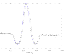
Figure 2: Demodulated drift scan of Jupiter (dots) and acquired drift-scan (dot-dash), with fitted minima and maximum (short continuous). Increasing delay between the two are barely visible. Correction for declination and non-transit passage of source are conceptually drawn under the plots.

This procedure has been applied on all planet drift-scans with a moderate $\alpha$ angle (i.e.,  close to transit) so to have pronounced minima well above noise level. The beam-throw of our telescope has been calibrated to a value of $(22.1^{\prime}\pm 0.4^{\prime})/Vpp$ of the transducer. Stability of modulation angles during the drift scans is higher than 0.3%.

2.2 Correction for atmospheric absorption.

In order to correct for atmospheric absorption we measure zenithal channel transmissions ($\tau_{0}$) performing several skydips (chopping at focal plane between atmospheric signal and a Black-Body reference at telescope temperature) during each night and correcting for a secant-law at angles different from zenith. Altitude angles are stepped to match tenths of air-masses ($90$ for $1.0$, $65.24$ for $1.1$, ecc… ). Skydips data present themselves as continuous acquisition of an offset that varies at the change of telescope elevation. Averages of each plateau continuous acquisition are subsequently fitted with a $1/\cos h$ law. As expected there is good agreement with air-mass dependence and we obtain transmission values for zenithal angle $z$:

$$T=\biggl{(}1-\frac{\rho}{\cos(90-h)}\biggr{)}$$ (6)

where $1-\rho$ is zenithal transmission, and $h$ is telescope elevation. Typical atmospheric transmission values for the four channels are listed in table 1.

Table 1: Values for zenithal transmission of the 4 channels on jupiter drift night.

Channel	$\tau_{0}$
$1(143GHz)$	$0.853$
$2(212GHz)$	$0.866$
$3(271GHz)$	$0.812$
$4(353GHz)$	$0.651$

3 Beam shape reconstruction.

Having a correct knowledge of the modulation amplitude, we now focus on the exact beam-shape of our instrument. By technical design, we employ a compact Cassegrain configuration with a 8 meter focal length and 40mm of correct focal plane we expect by design and ray-tracing a FWHM beam of 17 arcminutes. Yet, it is necessary to have an experimental evidence of the beam-shape of photometer+telescope (the beam shape of the photometer alone has been measured in laboratory). An exact reconstruction of the beam shape allows us to reduce the contribution to calibration uncertainty regarding instrumental errors (for planet temperature see 4.1).

The responsivity of the different spectral channels, when measuring CMB anisotropies, is defined by eq.7. The two major uncertainties in this quantity are the planet temperature considered as the integrated black-body temperature over the frequency bands of the instrument, and the $\Omega_{beam}$ of the telescope, that is exactly expressed by eq.8

$$R(\mu K/nV)=\frac{T_{CMB}}{S_{planet}}\frac{\Omega_{planet}}{\Omega_{beam}}\frac{\int BB(T_{planet},\nu)f(\nu)d\nu}{\int BB(T_{CMB},\nu)\frac{xe^{x}}{e^{x}-1}f(\nu)d\nu}$$ (7)

$$\Omega_{beam}=\int\int\sin\theta\cos\theta\cdot AR(\theta,\phi)d\theta d\phi$$ (8)

where $BB(T,\nu)$ is the blackbody emission (brightness), and $AR(\theta,\phi)$ is the angular response of the instrument that in our case can be considered cilindrically simmetric (i.e.,  function of $\theta$ alone).

3.1 Jupiter drifts.

One of the most bright and point-like sub-millimetric sources frequently adopted is Jupiter. The best way to determine the beam-shape would be to drift-scan at various declination offsets while chopping the source with a black-body reference, but unfortunately atmospheric fluctuations (which would not be removed), having a large ($\sim 16^{\prime}$) beam, dwarf the diluted planet signal. Consequently we simulate the drift-scan acquisition, introducing lock-in integration and correct modulation by the acquired LVDT and pointing system. Each beam-model generates a different convolved map from which the drift is extracted. All drifts thus obtained are best-fitted to the real time-ordered data (hereafter TOD) acquired. The advantage of this simulation is the capacity of considering any degree of sidelobe contamination during modulation if beamsize and half beam-throw are comparable.

Resulting fits thus obtained define the best beam-shape for each spectral channel. Solid angle $\Omega_{beam}$ present in eq.7 can then be computed by simple numerical integration. Moreover, the different angular responses of the various channels may induce differences in the ratios of atmospheric fluctuations as they cross the observed sky patch, differences that have to be accounted for during calibration. One important issue is that the main beam and the reference beam do not differ in the manner that contour levels of the beam are similar and do not undergo deformations. This has been verified confronting the simulated drift obtained by the afore-mentioned procedure, and the following method to construct the reference beam shape. This method is possible if data from a very small parallactic angle $p$ is used. In our case 3 square-field modulation allows us to reconstruct the reference beam by rescaling the negative sidelobe at the beginning of the drift scan. This can be done because contamination from the main beam is lower than -50dB at distances greater than half beamthrow. A third method to obtain the original beamshape is to generate families of analytical beamshapes B(x) and simulate passage of the source by calculating the contamination level for every data point as in (eq.9):

$$Data(x)=B(x)-\frac{1}{2}B(\sqrt{x^{2}+m_{A}^{2}-2xm_{A}\cos p})$$ (9)

Beam shapes obtained with different methods are consistent, and FWHM obtained is equal to $16^{\prime}\pm 1^{\prime}$.

Figure 3: Relative differences of the 4 spectral channels over-plotted for Jupiter drifts (top) and moon scans (bottom).

Moreover it is important to note that relative differences in the beamshape, that can slightly alter the data on planet drifts, is a negligible effect while studying beam-sized sources. Cross scans performed on the moon with our instrument report very low relative difference between different spectral channels (after intensity peak-normalization). In fig. (3) relative differences (i.e. difference of normalized scans - baseline $=0$, peak emission $=1$ - between spectral channels) of Jupiter drifts and Moon scans can be seen in the double plot. This allows us to consider the same form-factor for all 4 channels in the analysis of the galaxy cluster SZ-effect performed (De Petris et al. 2002).

4 Refinement of optical calibrations.

When detecting CMB anisotropies or indeed any cosmological signal it is necessary to convert the voltage signal (amplified bolometer output) to CMB thermodynamic temperature or power. To do so, a good knowledge of the optical responsivity $R=\Delta T/\Delta V$ is required. The best method to determine this physical parameter would be of course, to measure the same signal that is our final measuring objective but of which we already know its value (i.e. CMB dipole for CMB experiments and so on…) This is not always possible, so we restrain ourselves to dividing possible calibrations in two different sets: point-like sources (total-flux gathering), or extended sources (beam-dependent).

4.1 Planet models.

Many models of planetary emission have been proposed and subsequently refined with many different spectroscopic measurements in the recent past (Ulich 1973), (Furniss et al. 1977), (Werner et al. 1978), (Whitcomb et al. 1978), (Hildebrand et al. 1985), (Griffin et al. 1986), (Mangum 1992), (Naselsky et al. 2003). All these measurements have been plotted in figure fig.4, along with the thermal model with modified Van-Vleck Weisskopf line profiles assumed by Moreno (Moreno, 1998). Moreover spectral absorption lines are expected from the nominal synthetic spectra of Jupiter at the HCN (J=1 and J=2) and PH3 (J=0) frequencies. The latter two should be practically indistinguishable by a $\sim 10\%$ bandwidth filter as the ones we employed. The variability of Jupiter’s emission is known at low frequencies to be connected to synchrotron emission relative to spiraling particles of solar wind in Jupiter’s magnetic field. Although dominant at radio frequencies ($<10GHz$) this contribution is negligible in the sub-mm region. The large uncertainties in the existing Jupiter temperature measurements hint to a possible apparent thermal variation, as noted in (Naselsky et al. 2003), yet this could be the case if narrow spectral bands were employed and local variations in chemical composition distribution were present, altering the relative absorption of the lines. In our case, integration over our spectral channels, and spatially over the whole planet, would dilute this variation at less than a few percent effect. Lack of information, obtainable with future repeated measurements at different time-scales with narrow-band spectrometers, could resolve this uncertainty that leaves us with a $10\%$ error on the thermal temperature of Jupiter used for calibrating our detectors. These temperatures are for the 4 channels: 171, 171, 170 and 169K respectively for the 143, 213, 272 and 353 GHz.

Figure 4: Jupiter temperature measures from (see text references) different experiments. Over plotted is the thermal emission with Van-Vleck modified profiles as in (R.Moreno ph.D. thesis 1998). Over plotted are Fotomito spectral channels over which integration is computed for calibration.

Substituting all quantities calculated and the total $\Omega$ of the best-fitted beam in 7 we obtain the revised responsivities for the four spectral channels : $(462\pm 46)\mu k/nV$, $(377\pm 46)\mu k/nV$, $(426\pm 43)\mu k/nV$ and $(317\pm 32)\mu k/nV$. Ten percent errors have been considered due to jupiter temperature uncertainty, widely dominant as error source.

5 Geometrical form factors for cluster observations.

It has been mentioned before that the characterization of the beam profile and determination of actual modulation pattern and amplitude into the sky are vital to retrieve accurate calibration data from the observation of point-like sources. Besides, they also allow correct interpretation of observational data when significantly extended sources are scanned; this is the case for the measurement of SZ effect towards galaxy clusters (which exhibit typical angular sizes of up to tens of arcminutes), where signal recovery from noisy datasets can obviously take full advantage from the characterization of filtering and selection effects provided from the observation strategy. It has been noted (see eq. 7) that the effective brightness map observed from the experiment when exploring a given sky region will suffer from the dilution/smoothing effects due to the finite angular resolution of the experiment:

$$S_{\nu}(\alpha_{0},\delta_{0})=\int_{\alpha,\delta}B_{\nu}(\alpha-\alpha_{0},\delta-\delta_{0})AR(\alpha,\delta)d\Omega$$ (10)

since, even at few tens of arcminutes away from the source center, the collected signal will not be negligible, it turns out that at a given modulation amplitude $\theta_{BT}$, a differential measurement will be partially reduced from the contamination effect in the side beams of the modulation pattern. It is therefore necessary to distinguish between the observed SZ effect, as the apparent CMB anisotropy that results from the difference between beam-diluted signals in center and partially contaminated reference beams at beam-throw $\theta_{BT}$, and the central value of the comptonization across the cluster, as it would be measured in absence of side beam contamination and in pencil beam conditions. The two quantities, in term of the measured CMB comptonization effect, are related by

$$\Delta T^{obs}=\Delta T_{0}^{dil}-\Delta T^{dil}_{\theta_{BT}}=\eta\Delta T_{0}$$ (11)

where $\eta$ plays the role of a geometrical form factor needed to define the coupling between the instrument angular selection capabilities (i.e.,  angular response and modulation beam-throw) and the cluster morphology (e.g.,  the isothermal $\beta$-model parameters when such modeling is justified from X-ray observation). Figs. 5 and 6 show the dependence of the form factor from beam-throw and cluster core radius respectively, assuming the present single-pixel resolution of $16^{\prime}$ FWHM. Obviously, reference beam contamination decreases with increasing beam-throws (fig.5), and at any fixed beam-throw the form factor is maximized for a certain specific core radius representing a balance between reduction of signal dilution and reference beam contamination, so that, basically, one should try to reach the highest possible modulation amplitude for any selected cluster.

Figure 5: Form factor dependence from beam-throw, when $3$-field modulation is applied. MITO telescope resolution ($16^{\prime}$ FWHM) has been considered. A core radius of $8^{\prime}$ has been assumed.

Figure 6: Form factor variation as a function of core radius for the MITO telescope (FWHM $16^{\prime}$), with the $\pm 20^{\prime}$ $3$-field modulation pattern applied during the Coma observations. A value of $\beta=0.75$ has been assumed, in accordance with X-ray measurements on the same cluster. The selected modulation amplitude ensures optimal efficiency ($\eta\simeq 0.4$) for $\theta_{core}\simeq 10^{\prime}$ as for Coma.

More realistically, a compromise is to be found between maximization of the form factor and removal of bulk atmospheric fluctuation, which is more efficient when modulation explores sky regions close to that of the main beam. The above considerations have been usefully applied to evaluate $\eta$ in the case of the Coma cluster, with the $\beta-$model parameters $b=0.75\pm 0.03$ and $\theta_{c}=10.5^{\prime}\pm 0.2$, the beam profile reconstructed with the procedure described in 3 and a beamthrow of $\pm 18.5^{\prime}$, we get $\eta=0.43\pm 0.02$ which is compatible, within errors, with the determination of $0.41\pm 0.02$ reported in De Petris et al. , 2002.

References

- [1] \harvarditem(De Petris et al.)(1996)depetris96De Petris M., E. Aquilini, M. Canonico, L. D’Addio, P. de Bernardis, G. Mainella, A. Mandiello, L. Martinis, S. Masi, B. Melchiorri, M. Perciballi and F. Scaramuzzi 1996, New Astr., 1, 121
- [2] \harvarditem(De Petris et al.)(2002)depetris2002 M. De Petris, L. D’Alba, L. Lamagna, F. Melchiorri, A. Orlando, E. Palladino, Y. Rephaeli, S. Colafrancesco, E. Kreysa, M. Signore 2002, Astroph.J. , 574, L119
- [3] \harvarditem(Furniss et al.)(1977)Furniss77 Furniss I., Jennings R.E. and King K.J., 1977, Icarus, 35, 74
- [4] \harvarditem(Griffin et al.)(1986)Griffin86 Griffin M.J., Ade P.A.R., Orton G.S., Robson E.I., Gear W.K. and Nolt I.G. and Radostitz J.V., 1986, Icarus, 65, 244
- [5] \harvarditem(Hildebrand et al.)(1985)Hildebrand85 Hildebrand R.H., Loewenstein R.F., Harper D.A., Orton G.S., Keene J. and Whitcomb S.E., 1985, Icarus, 64, 64
- [6] \harvarditem(Lamagna et al.)(2002)lamagna2002 Lamagna L., De Petris M., Melchiorri F., Battistelli E. S., De Grazia M., Luzzi G., Orlando A., Savini G., 2002, AIP Conference Proceedings, 616, 92, editors: M. De Petris and M. Gervasi
- [7] \harvarditem((Mainella et al.)(1996)Mainella96 Mainella G., P. de Bernardis, M. De Petris, A. Mandiello, M. Perciballi and G.Romeo 1978, Applied Optics , 35, 2246
- [8] \harvarditem(Mangum )(1992)Mangum92 Mangum J.G., 1993, Astr. Soc. of the Pacific, 105, 117
- [9] \harvarditem(Melchiorri et al.)(1996) mel96 Melchiorri, B., De Petris, M., D’Andreta, G., Guarini, G., Melchiorri, F. and Signore, M. 1996, Astroph.J. , 471, 52
- [10] \harvarditem(Moreno )(1998)Moreno98 Moreno R., PhD Thesis, 1998, University Paris VI
- [11] \harvarditem(Naselsky et al.)(2003)Naselsky03 Naselsky P.D., Verkhodanov O.V., Christensen P.R., and L.Y. Chiang, Astronomy and Astrophysics, accepted for pubblication.
- [12] \harvarditem(Ulich )(1973)Ulich73 Ulich B.L. 1973, Icarus, 21, 254
- [13] \harvarditem(Werner et al.)(1978)Werner78 Werner M.W., Neugebauer G., Houck J.R. and Hauser M.G., 1978, Icarus, 35, 289
- [14] \harvarditem(Whitcomb et al.)(1978)Whitcomb78 Whitcomb S.E., Hildebrand R.H., Keene J., Stiening R.F. and Harper D.A., 1978, Icarus, 38, 75
- [15]