The Extremely Metal-Poor, Neutron-Capture-Rich Star CS 22892-052: A Comprehensive Abundance Analysis

Abstract

High-resolution spectra obtained with three ground-based facilities and the Hubble Space Telescope (HST) have been combined to produce a new abundance analysis of CS 22892-052, an extremely metal-poor giant with large relative enhancements of neutron-capture elements. A revised model stellar atmosphere has been derived with the aid of a large number of Fe-peak transitions, including both neutral and ionized species of six elements. Several elements, including Mo, Lu, Au, Pt and Pb, have been detected for the first time in CS 22892-052, and significant upper limits have been placed on the abundances of Ga, Ge, Cd, Sn, and U in this star. In total, abundance measurements or upper limits have been determined for 57 elements, far more than previously possible. New Be and Li detections in CS 22892-052 indicate that the abundances of both these elements are significantly depleted compared to unevolved main-sequence turnoff stars of similar metallicity. Abundance comparisons show an excellent agreement between the heaviest $n$-capture elements (Z $\geq$ 56) and scaled solar system $r$-process abundances, confirming earlier results for CS 22892-052 and other metal-poor stars. New theoretical $r$-process calculations also show good agreement with CS 22892-052 abundances as well as the solar $r$-process abundance components. The abundances of lighter elements (40 $\leq$ Z $\leq$ 50), however, deviate from the same scaled abundance curves that match the heavier elements, suggesting different synthesis conditions or sites for the low-mass and high-mass ends of the abundance distribution. The detection of Th and the upper limit on the U abundance together imply a lower limit of 10.4 Gyr on the age of CS 22892-052, quite consistent with the Th/Eu age estimate of 12.8 $\pm$ $\simeq$ 3 Gyr. An average of several chronometric ratios yields an age 14.2 $\pm$ $\simeq$ 3 Gyr.

1 INTRODUCTION

Elemental abundance observations of Galactic halo stars provide fundamental knowledge about the history and nature of nucleosynthesis in the Galaxy. In particular, abundance determinations of the neutron-capture ($n$-capture) elements — those from the ($s$)low and ($r$)apid neutron-capture processes — have been utilized to constrain early Galactic nucleosynthesis and chemical evolution. A number of observational and theoretical studies have, for example, established that at the earliest times in the Galaxy the $r$-process was primarily responsible for $n$-capture element formation (Spite & Spite 1978; Truran 1981; Sneden & Parthasarathy 1983; Sneden & Pilachowski 1985; Gilroy et al. 1988; Gratton & Sneden 1994; McWilliam et al. 1995; Cowan et al. 1995; Sneden et al. 1996, Ryan, Norris & Beers 1996). The onset of the $s$-process occurs at higher metallicities (and later Galactic times) with the injection of nucleosynthetic material from long-lived low- and intermediate-mass stars into the interstellar medium (Busso, Gallino, & Wasserburg 1999; Burris et al. 2000). The relatively recent detections of radioactive elements such as thorium and uranium in a few $r$-process-enhanced metal-poor stars are providing new opportunities to determine the ages of the oldest stars, and in the process, set lower limits on the age of the Galaxy (Sneden et al. 1996; Cowan et al. 1997, 2002; Johnson & Bolte 2001; Cayrel et al. 2001; Hill et al. 2002; Schatz et al. 2002).

The halo giant star CS 22892-052 was discovered in the southern Galactic pole survey of Beers, Preston, & Shectman (1985, 1992), and was judged to be extremely metal-poor based upon the relative weakness of its Ca II K line. Basic data for this star are listed in Table 1. McWilliam et al. (1995) included CS 22892-052 in a followup high-resolution chemical composition study of 33 low metallicity stars. Inspection of the CS 22892-052 spectrum revealed unusually strong transitions of $n$-capture elements, and so Sneden et al. (1994) subjected it to a separate analysis. That study confirmed the status of CS 22892-052 as an extremely metal-poor giant (T_eff $\approx$ 4725 K, log $g$ $\sim$ 1.0, [Fe/H] $\sim$ –3.1). The low signal-to-noise (S/N) and moderate spectral resolution of their data permitted study of only the stronger $n$-capture spectral features of (mostly) the rare-earth elements. But Sneden et al. established that CS 22892-052 is indeed $n$-capture-rich (e.g., [Eu/Fe] $\approx$ +1.6), and that the relative abundances of nine elements in the range 56 $\leq$ Z $\leq$ 66 are consistent with a scaled solar-system purely $r$-process distribution. Norris, Ryan, & Beers (1997a) performed an independent study of this star and found abundances consistent with the Sneden et al. investigation.

A more extensive spectroscopic study of CS 22892-052 with better data (Sneden et al. 1996) expanded the total number of $n$-capture element abundances to 20, including a clear detection of the strong Th II 4019 Å line. Thorium is radioactive with a half-life of 14.0 Gyr, and the observed [Th/Eu] abundance ratio combined with an assumed extrapolation of the solar-system $r$-process abundance distribution out to Th yielded a simple “decay age” of about 15 Gyr. Unfortunately CS 22892-052 is also relatively carbon-rich ([C/Fe] $\approx$ +1.0; McWilliam et al. 1995). A study of carbon-rich metal-poor stars without $r$-process abundance enhancements (Norris, Ryan, & Beers 1997b) revealed an important problem in using the Th II 4019 Å line for chronometry estimates: this is a transition blended with not only atomic contaminants but also two ¹³CH lines. All these contaminants must be properly accounted for in the extraction of the Th abundance in CS 22892-052.

Most strong $n$-capture element transitions in the spectra of metal-poor giants occur at wavelengths $\lambda$ $<$ 4300 Å. Therefore we obtained a new high resolution, high signal-to-noise (S/N) near-UV spectrum of CS 22892-052 with the Keck I HIRES. Preliminary abundances from that spectrum were reported by Sneden et al. (2000). Spectroscopic data farther in the UV were gathered with the Hubble Space Telescope Imaging Spectrograph (STIS). New visible wavelength spectra have been obtained with the McDonald Smith 2.7-m telescope and “2d-coudé” spectrograph. Commissioning data with the ESO VLT/UT2 (Kueyen) and the UVES spectrograph have also been included in this assemblage. With these four data sets we have performed a new abundance analysis of CS 22892-052. Abundances or significant upper limits are reported for 57 elements in this star. To date this is the largest number of elemental abundances discussed for any star other than the Sun, rivaled only by the 54 elements detected by Cowley et al. (2000) in the Ap star HD 101065 (Przybylski’s star). Observations are described in §2, the abundance analysis is given in §3, and our interpretation of this large abundance set is discussed in §4.

2 OBSERVATIONS AND REDUCTIONS

HST STIS UV spectra: We obtained high-resolution spectra in the vacuum ultraviolet, 2400 $\leq$ $\lambda$ $\leq$ 3100 Å, with the Hubble Space Telescope Imaging Spectrograph ($STIS$). The instrument setup included echelle grating E230M centered at $\lambda$ = 2707 Å, entrance aperture 0.2$\arcsec\times$0.06$\arcsec$, and the $NUV-MAMA$ detector. The resolving power ($R$ $\equiv$ $\lambda/\Delta\lambda$) was approximately 30,000. Because CS 22892-052 is a ($V$ = 13.1) K-giant star, 12 separate HST visits with five individual integrations each were needed to produce a final reduced spectrum with S/N $\sim$ 20. We employed standard HST STIS reduction procedures implemented in IRAF to combine the 60 integrations into a one-dimensional, flat-fielded, wavelength-calibrated spectrum. The individual spectra from each of the 60 integrations had very low S/N values, and experiments with the total reductions showed that a more reliable final spectrum could be obtained with background corrections neglected. We therefore used the “raw” STIS spectra, and combined these 60 with a median algorithm that neglected the five highest and five lowest data points in each spectral pixel.

Keck I Near-UV spectra: We gathered Keck I $HIRES$ (Vogt et al. 1994) echelle spectra in the spectral region 3100 $\leq$ $\lambda$ $\leq$ 4250 Å. Seven individual integrations were combined to produce the final spectrum. The resolving power of the fully reduced spectrum was $R$ $\simeq$ 45,000. Its S/N decreased blueward, from $\sim$150 per pixel at $\lambda$ $\sim$ 4200 Å to $\sim$20 at $\lambda$ $\sim$ 3100 Å; both the stellar flux and the CCD response decline toward the UV. We used auxiliary tungsten lamp spectra for flat-fielding the stellar spectrum and Th-Ar lamp spectra for wavelength calibration. We performed all extraction and reduction tasks to produce a spectrum for analysis with the software package MAKEE (e.g., Barlow & Sargent 1997).

McDonald 2d-coudé spectra: We obtained a high-resolution spectrum in the wavelength range 4300 $\leq$ $\lambda$ $\leq$ 9000 Å with the McDonald Observatory 2.7m H. J. Smith telescope and “2d-coudé” echelle spectrograph (Tull et al. 1995). In addition to tungsten and Th-Ar calibration spectra, we also acquired a spectrum of the hot, rapidly rotating star $\lambda$ Aql for use in canceling telluric (O₂ and H₂O) lines that occur in the yellow-red region. The spectrograph setup had a 1.2$\arcsec$ entrance slit and a Tektronix 2048$\times$2048 CCD detector, yielding a 2-pixel resolving power of $R$ $\simeq$ 60,000. The star was observed on three consecutive nights. Initial processing of the raw spectra was done with standard $IRAF$ echelle reduction tasks. The co-added reduced spectra have S/N $>$ 100 for $\lambda$ $>$ 5500 Å, and this declines steadily to levels of $\sim$40 at $\lambda$ $\sim$ 4400 Å.

VLT UVES spectra: We made use of VLT UVES (Dekker et al. 2000) echelle spectra which were obtained during the commissioning phase of the instrument and during the course of the ESO Large Program 165.N-0276(A) (First Stars, PI R. Cayrel). The two sets of observations obtained using a dichroic beam-splitter covered respectively 3300-4000 Å + 4800-10000 Å (at a resolution of $R$ $\approx$ 55000) and 3350-4570Å + 6700-10000Å ($R$ $\approx$ 45000), for a total of 5.5 hours of integration. The spectra were reduced individually, using a MIDAS (Warmels 1991 and references therein) context dedicated to UVES, including bias and inter-order background subtraction, optimal extraction of the object (weighted over the profile object profile), flat-field correction and a wavelength calibration using a Th-Ar lamp. The S/N of the combined spectra ranged from $\sim$40 at 3300Å to $\sim$100 at 4500Å in the blue part of the spectrum, and $\sim$175-200 throughout most of the red part.

Final processing of the spectra: We used the software package $SPECTRE$ (Fitzpatrick & Sneden 1987) for the completion of the stellar data reductions, to $(a)$ eliminate anomalous radiation events and bad pixels; $(b)$ normalize spectral continua with spline function fits to interactively chosen continuum points; and $(c)$ smooth the spectra via 2-pixel FWHM Gaussian convolutions for STIS, McDonald, and those parts of the Keck spectra with $\lambda$ $<$ 3400 Å. For unblended spectral lines, equivalent widths (EWs) were measured by fitting Gaussian profiles or by direct integrations over the absorption profiles. Line data for transitions used in this study are given in Table 2 for lighter (Z $\leq$ 30) elements, and in Table 3 for $n$-capture elements. Many lines are blended and/or have multiple sub-components, so synthetic spectra described in the next section were used instead of EWs for the abundance computations. There are two categories of such complex spectral features. Some of them (e.g., Ba II 4554.03 Å, La II 4086.71 Å, or Tb II 3702.85 Å) are sufficiently strong and unblended that measurement of an approximate EW was possible. For those lines the EW entries are written as “syn(EW)” so that the reader may have an indication of the absorption strengths. However, these EWs were not and should not be employed in abundance computations for CS 22892-052892. Other synthesized transitions are either so weak or so blended that EW measures would be meaningless and misleading. For those lines the EW entries are simply “syn”.

3 ABUNDANCE ANALYSIS

3.1 Model Atmosphere and Abundances of Lighter Elements

Spectral lines of Fe-peak species were employed in deriving a new model atmosphere for CS 22892-052. A conventional LTE analysis was performed in the same manner as was done in our earlier abundance analyses of $n$-capture-rich, very metal-poor stars (e.g., Westin et al. 2000; Cowan et al. 2002). We began with the line list of Westin et al. for species with Z $\leq$ 30, augmenting it to include lines of additional Fe-peak species rarely employed in abundance analyses (e.g., Sc I, Mn II). Single-line EW matches were employed for most transitions, but full spectrum syntheses were done for transitions of Sc I, Sc II, Mn I, Mn II, and Cu I, all of which have substantial hyperfine substructures (hfs).

The effective temperature, T_eff, was determined by minimizing the line-to-line abundance differences with excitation potential, EP, for species with a sufficient EP range. The microturbulent velocity parameter, v_t, was adjusted to remove trends in line abundances with EW. The gravity, log $g$, was set by requiring neutral and ionized species of Sc, Ti, V, Cr, Mn, and Fe to have the same abundances on average.

Trial model atmospheres for CS 22892-052 were interpolated from the Kurucz (1995) grid with a modified version of software kindly provided by A. McWilliam (private communication). Models without convective overshooting were chosen, as recent literature suggests that such models give best overall matches to optical and UV spectra of metal-poor stars (e.g., Castelli, Gratton, & Kurucz 1997; Peterson, Dorman, & Rood 2001). Abundances were computed for each line with the current version of Sneden’s (1973) line analysis code, iterating on the model parameters until the satisfaction of the above criteria was achieved. The best model had parameters (T_eff, log $g$, [M/H], v_t) = (4800$\pm$75 K, 1.5$\pm$0.3, –2.5, 1.95$\pm$0.15). The chosen model metallicity, [M/H] = –2.5, is somewhat larger than the derived [Fe/H] = –3.1, but –2.5 is the lowest metallicity of the Kurucz grid models without convective overshooting. Test abundance runs using models with overshooting and smaller model metallicities yielded little differences in derived model parameters.

Our spectroscopically-derived model atmosphere for CS 22892-052 is in good accord with low-resolution indicators. Extensive photometric temperature scales for giant stars have been determined by Alonso, Arribas, & Martinez-Roger (1999, 2001). We used their formulas with the photometric data of Table 1 to compute T_eff values for color indices $U-V,B-V,V-K,J-H$, and $J-K$ (the $V-R$ color is not covered by the Alonso formula). Giving the derived T_eff($V-K$) double weight due to the excellent temperature sensitivity of the $V-K$ color, we obtain: (a) $<\mbox{T${}_{\rm eff}$}>$ = 4791 $\pm$ 18 K ($\sigma$ = 44 K) if $E(B-V)$ = 0.00 (Beers et al. 1999); (b) $<\mbox{T${}_{\rm eff}$}>$ = 4836 $\pm$ 24 K ($\sigma$ = 58 K) if $E(B-V)$ = 0.02 (Beers et al. 1992), and (c) $<\mbox{T${}_{\rm eff}$}>$ = 4861 $\pm$ 27 K ($\sigma$ = 65 K) if $E(B-V)$ = 0.03 (from dust maps of Schlegel et al. 1998). All of these estimates agree well with the spectroscopic T_eff.

To compute an evolutionary gravity for CS 22892-052, fundamental physical considerations provide a standard formula relating absolute visual magnitude ($M_{V}$ = –0.2 $\pm$ 0.4, Beers et al. 1999), effective temperature (T_eff = 4800 $\pm$ 75 K), mass (assumed here to be a metal-poor near-turnoff mass $\mathcal{M}$ = 0.75 $\pm$ 0.10 $\mathcal{M}_{\odot}$), and bolometric correction (BC = –0.39 $\pm$ 0.04, computed from Eq. 18 of Alonso et al. 1999):

$$\log g_{evol}=-12.50+0.4\left(M_{V}+BC\right)+\log\mathcal{M}+4\log\mbox{T${}_{\rm eff}$}\$$

These quantities combine to yield log $g$_evol = 1.85 $\pm$ 0.25, in agreement with our derived log $g$_spec = 1.5 $\pm$ 0.3, given the uncertainties of both values.

Note that log $g$_spec $<$ log $g$_evol is in the expected sense if the ionization equilibrium used to constrain log $g$_spec is affected by “overionization” departures from LTE. However, the close agreement of abundances from neutral and ionized species of six different Fe-peak elements (with ionization potentials that range from 6.8 to 7.9 eV) indicates that our derived spectroscopic gravity is sufficient to compute reliable relative abundances of elements with only one ionization state or the other detected in CS 22892-052. Exceptions may exist for neutral species of elements with very low first ionization potentials (I.P. $\lesssim$ 5 eV); see remarks for K I below.

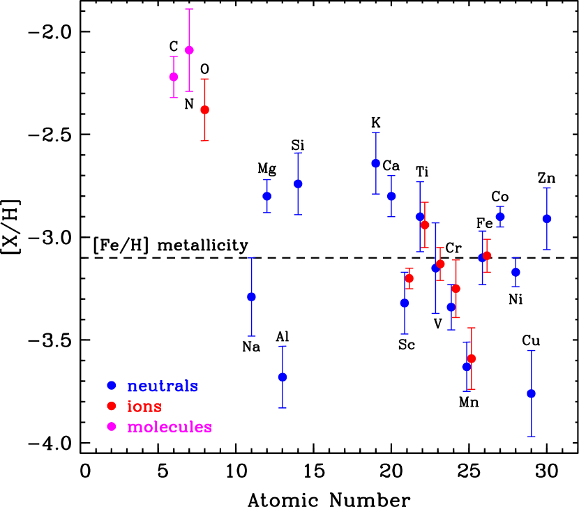
Figure 1: Abundances with respect to the Sun, [X/H], versus atomic number for elements with Z $\leq$ 30. The symbols are defined in the figure legend, and the dashed line representing the standard “metallicity” of CS 22892-052 is drawn through the Fe I abundance, [Fe/H] = –3.10. See §3.1 for discussion of the error bars displayed in this and other figures. For display purposes small leftward and rightward shifts for points from neutral and ionized species, respectively, have been imposed on abundances of elements represented by two ionization stages.

Derived abundances of elements with Z $\leq$ 30 are listed in Table 4 and plotted in Figure 1. Solar abundances are taken from Grevesse & Sauval (1998). Following Cowan et al. (2002), the error bars in this figure are generally the sample standard deviations $\sigma$. However, minimum values were imposed, noting that the smallest line-to-line scatter for any species (of light or $n$-capture elements) with at least several measured lines is $\sigma$ $\sim$ 0.05 dex. Therefore for an abundance based on three or more lines, the plotted error bar is the maximum of its $\sigma$ and 0.05. For a species with two measured lines, the error bar is the maximum of its $\sigma$ and 0.10. For a species with only one line, $\sigma$ is undefined and so an arbitrary value of 0.15 is adopted as the error bar. In a few cases with only 1-2 lines for a species, we have increased the error bar even further to account for very uncertain $gf$ values, difficult line blending problems, etc.

In general the abundances displayed in Figure 1 conform to well-established patterns for these elements in very metal-poor halo stars (e.g., Cayrel 1996; McWilliam 1998). In particular, the $\alpha$ elements are all overabundant in CS 22892-052: $<$[Mg,Si,Ca,TiI,TiII/Fe] = +0.26 $\pm$ 0.04 ($\sigma$ = 0.08). The light odd-Z elements Na and Al are underabundant with respect to Fe. Among the Fe-peak elements, the now-well-established overabundance of Co and underabundances of Mn and Cu (perhaps Sc and Cr as well) are evident. Apparently Zn is also overabundant, as it is in some other stars of this metallicity (e.g., Primas et al. 2000c; Blake et al. 2001).

A few of these overall conclusions should be viewed with caution. We emphasize the inherent uncertainties of elemental abundances deduced from only one line, as in the cases of Al, Si, and Zn. Also, the Cu abundance of CS 22892-052 has been determined from the Cu I resonance lines at 3247 and 3274 Å, not from the 5105 Å line that is employed in most other studies of this element in metal-poor stars. Since the 5105 Å line cannot be detected on our CS 22892-052 spectra, the mapping of its Cu abundance onto [Cu/Fe] trends with metallicity (e.g., Mishenina et al. 2002) cannot be accomplished with confidence yet. The Al abundance is derived from the Al I 3961 Å resonance line, which is known (e.g., Ryan et al. 1996) to yield systematically lower abundances than do the red-region spectral lines arising from excited states of this species. Finally, the large overabundance of K derived here may or may not be real. Takeda et al. (2002) have made statistical equilibrium calculations of the K I 7699 Å line strengths in stars of various metallicities, concluding that LTE-based [K/Fe] values are generally too large by 0.2 to 0.7 dex. Further investigation of this issue is warranted, but it is beyond the scope of the present investigation.

Next we consider the CNO element group. The [O I] 6300.3 Å line is detected on our VLT spectrum, but it is extremely weak, EW = 1.9 $\pm$ 0.2 mÅ. The line does not appear to be contaminated by telluric features. A synthetic spectrum fit to this spectral region was used to estimate the O abundance, and to ensure that reasonable abundances could be recovered from the comparably weak neighboring Fe I 6301.5, 6302.5 Å lines. The derived abundance, [O/Fe] $\approx$ +0.7, is in good agreement with abundances determined from [O I] lines in other very low metallicity giant stars (e.g.. Westin et al. 2000; Depagne et al. 2002). However, the Grevesse & Sauval (1998) recommended value of log $\epsilon_{\sun}$(O) = 8.83 has recently been re-assessed by Reetz (1999), Allende Prieto, Lambert, & Asplund (2001) and Holweger (2001); the mean of their values is log $\epsilon_{\sun}$(O) = 8.75. Adoption of this solar O value of course would increase the relative abundance in CS 22892-052 to [O/Fe] $\approx$ +0.8. It is recommended that the [O I] 6300 Å be re-observed in CS 22892-052 with better resolution and S/N (the 6363 Å line is a factor of three weaker, and likely to remain undetected in this star).

The anomalous strength of the CH G-band in CS 22892-052 was first discovered from a medium-resolution spectrum of this star, and noted in Table 8 of Beers et al. (1992). The implied large C abundance was confirmed in subsequent high-resolution studies (Sneden et al. 1996; Norris et al. 1997a). Our synthetic spectrum fits to G-band lines recover the earlier results. But as with O, the solar abundance of C may need revision, as a new analysis of the [C I] 8727 Å line by Allende Prieto, Lambert, & Asplund (2002) yields log $\epsilon_{\sun}$(C) = 8.39, about 0.1 dex smaller than the value recommended by Grevesse & Sauval (1998) (however, Holweger 2001 recommends log $\epsilon_{\sun}$(C) = 8.59). This of course would lead to a comparable upward shift in our derived [C/Fe] = 0.95, but a careful analysis of the CH G-band in both the Sun and CS 22892-052 should be done before altering the [C/Fe] listed in Table 4.

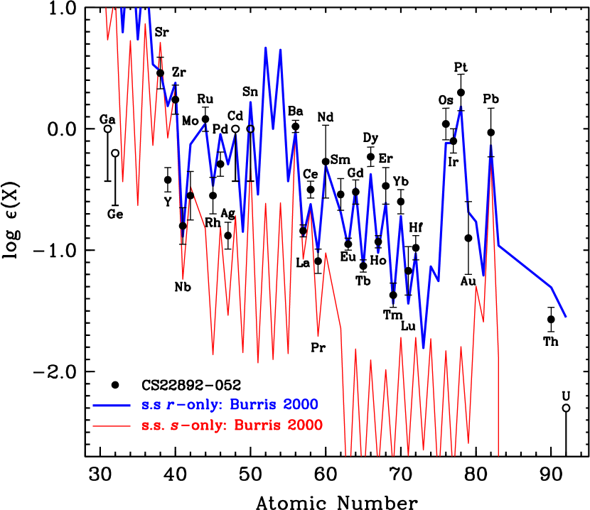
Figure 6: Observed $n$-capture abundances in CS 22892-052 and two scaled solar-system abundance distributions (Burris et al. 2000). Detected elements are shown as solid circles with complete error bars, and upper limits are denoted with open circles with only the lower half of an arbitrary-length error bar. The solar-system $r$-process abundance set (solid line) is vertically scaled by a single additive constant to match the observed Eu abundance, while the $s$-process set (dashed line) is scaled to match the observed Ba abundance.

Norris et al. (1997b) searched without success for ¹³CH features on their spectra of CS 22892-052, and suggested that ${\rm{}^{12}C/^{13}C}$ $\gtrsim$ 10. Using the Sneden et al. (1996) CTIO 4-m echelle spectrum, Cowan et al. (1999) estimated ${\rm{}^{12}C/^{13}C}$ $\approx$ 16, From the new VLT spectrum we concur with the earlier value, deriving ${\rm{}^{12}C/^{13}C}$ = 15 $\pm$ 2. Additionally, CN blue system $\Delta$v = 0 bandheads are weakly visible in CS 22892-052 (see Figure 6 of Sneden et al.). New syntheses of the 3868-3885 Å region of our Keck HIRES spectrum yield approximately the same N enhancement ([N/Fe] $\approx$ +0.8) as was claimed in the earlier work.

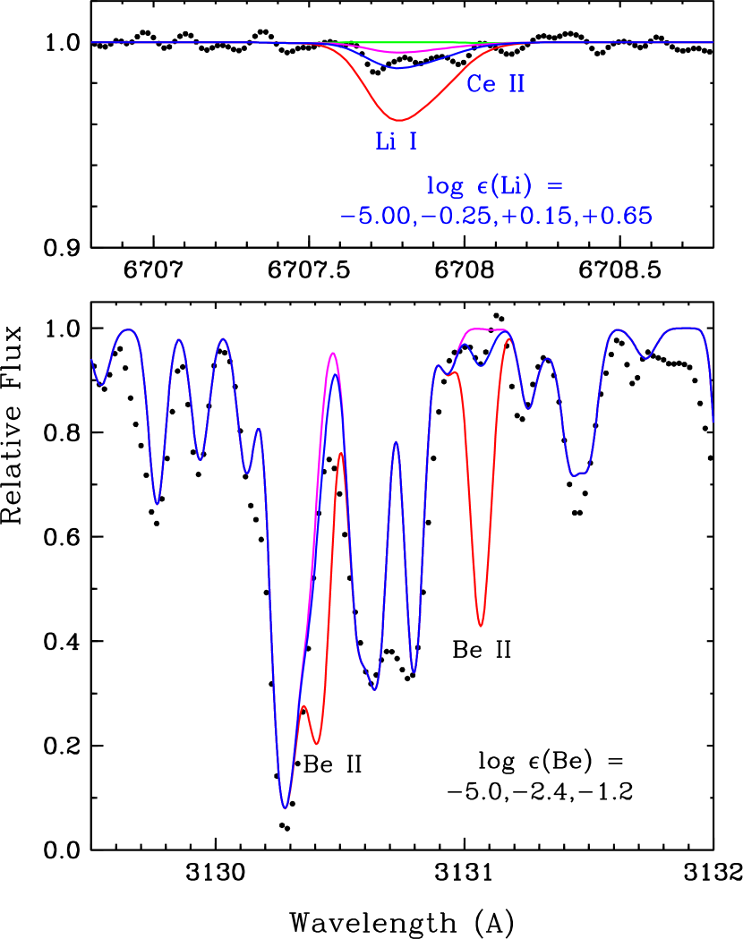
Figure 2: Observed and synthetic spectra of the Li I and Be II resonance doublets in CS 22892-052. In the upper panel, a potential Ce II blending transition at 6708.10 Å is marked. The synthetic spectra are computed with log $\epsilon$(Li) = –5.0 (dotted line), –0.25 (short dashed line), +0.15 (solid line), and +0.65 (long dashed line). In the lower panel, the synthetic spectra are chosen to illustrate the appearance of the spectrum without the presence of Be (log $\epsilon$(Be) = –5.0, dotted line), the appearance if Be were assumed to be undepleted (log $\epsilon$(Be) = –2.4, dashed line), and the best-fit to the 3131 Å feature (log $\epsilon$(Be) = –1.2, solid line). See §3.1 for further comment on the Li and Be features.

Finally, we comment on Li and Be abundances, listed in Table 4 but not plotted in Figure 1. These two elements are normally destroyed in stellar interiors during evolution beyond the main sequence, so their present abundances in CS 22892-052 are unlikely to reflect the values of the ISM from which this star formed. The Li I 6707.8 Å resonance doublet is tentatively detected in our VLT spectrum, with EW = 3.5 $\pm$ 0.5 mÅ. Synthetic spectrum fits, using the Ca I 6717.69 Å line to align the wavelength scales of the observed and synthesized spectra, and with no ⁶Li included in the syntheses, yielded log $\epsilon$(Li) $\approx$ +0.15. We show the Li I doublet spectrum in the upper panel of Figure 2. While it is possible to argue for lower Li abundances than we have estimated, much larger abundances are ruled out based on the extreme weakness of the observed feature. A new study of the 6707.8 Å feature in $s$-process-enriched post-AGB stars by Reyniers et al. (2002) suggests that all or part of this often-strong absorption may actually be due to a line of Ce II ($\lambda$ = 6708.099 Å, E.P. = 0.71 eV, log $gf$ = –2.12; Palmeri et al. 2000). We included this line in our syntheses, but (as shown in Figure 2) it is well separated from the Li I in the CS 22892-052 spectrum, and will create detectable line depth only if the Ce abundance is increased by factors of 5-10 more than our derived value. The Li abundance of CS 22892-052 is not unusual for a metal-poor giant star that has undergone convective envelope mixing, as several studies (e.g., Ryan & Deliyannis 1998, Gratton et al. 2000) find log $\epsilon$(Li) $\lesssim$ 0 for stars with similar atmospheric parameters.

The Be abundance in CS 22892-052 was determined from our Keck spectrum, using spectrum synthesis fits to the observed Be II 3130 Å doublet; see the lower panel of Figure 2. We used the line list assembled and extensively tested by Primas et al. (1997), fixing all abundances except Be to the values given derived in this paper. There are several $n$-capture species transitions that surround the Be II doublet: Ce II 3130.34 Å, Nb II 3130.78 Å, Gd II 3130.81 Å, Ce II 3130.87 Å. These lines are usually insignificant in normal dwarfs and subgiants, but do contribute to the total absorption in CS 22892-052. We derived log $\epsilon$(Be) = –2.4 $\pm$ 0.4 from the 3131.07 Å line. The large error estimate given in Table 4 is due to the combination of substantial line blending, the weakness of the Be II doublet, and the modest S/N of our spectrum in this region.

The Be abundance in CS 22892-052 is extremely low. Halo dwarf stars of similar metallicity typically have Be abundances about a factor of 10 larger. Two examples are: log $\epsilon$(Be) = –1.1 $\pm$ 0.2 in both G 64-12 ([Fe/H] = –3.3; Primas et al. 2000a) and LP 815-43 ([Fe/H] = –2.95; Primas et al. 2000b). Alternatively, using the Boesgaard et al. (1999) mean relationship between Be abundance and stellar metallicity, the predicted initial abundance for CS 22892-052 with [Fe/H] = –3.1 would be log $\epsilon$(Be) = –1.6. These zero-age Be values in very metal-poor stars indicate that significant internal Be depletion has occurred in CS 22892-052. For illustration we show in Figure 2 a synthetic spectrum with log $\epsilon$(Be) = –1.2; the observed 3131.07 Å and (highly blended) 3130.42 Å lines both clash badly with this “zero-age” Be abundance.

The low Be value in CS 22892-052, combined with the equally low Li abundance, may hint at the presence of a mixing mechanism that is able to affect both Li and Be at the same time. Detailed predictions of this phenomenon at low metallicities are lacking, but Boesgaard et al. (2001) show that depletion of both elements occurs in metal-rich F-type stars. Their observations yield a depletion correlation of $\delta$[log $\epsilon$(Be)] $\approx$ 0.36$\delta$[log $\epsilon$(Li)]. Assuming that CS 22892-052 began its life with a “Spite plateau” Li abundance of log $\epsilon$(Li) $\approx$ +2.0 (Ryan et al. 1999 and references therein) then for CS 22892-052 the observed log $\epsilon$(Li) = +0.15 implies $\delta$[log $\epsilon$(Li)] $\sim$ –1.9 or $\delta$[log $\epsilon$(Be)] $\sim$ –0.7. This prediction is in rough accord with the observed $\delta$[log $\epsilon$(Be)] $\sim$ –1.0.

Unfortunately, we cannot confidently predict the Be abundance that CS 22892-052 had at birth, because there may be significant star-to-star scatter among the lowest metallicity unevolved stars. For example, Primas et al. (2000b) derive log $\epsilon$(Be) $\leq$ –1.4 for CD –24^∘17504 ([Fe/H] = –3.3), at least a factor of two lower than that of G 64-12. This possible initial scatter, combined with a lack of extensive Be studies in metal-poor giants and lack of quantitative predictions for Be depletion in low metallicity stars, prevent us from drawing more quantitative conclusions about the Be abundance in CS 22892-052.

3.2 Abundances of the $n$-Capture Elements

Derivation of $n$-capture elements was accomplished with EW matches for lines that were either very weak (log(EW/$\lambda$) $\lesssim$ –5.3) or single $and$ unblended absorptions. For other transitions synthetic spectrum computations were used. All $n$-capture lines are listed in Table 3. Construction of atomic/molecular line lists for the synthetic spectra have been described in earlier papers (e.g., Sneden et al. 1996; Westin et al. 2000; Cowan et al. 2002). Laboratory studies in the past couple of decades have provided a wealth of accurate transition probabilities, hfs constants, and isotopic wavelength shifts for many $n$-capture-element neutral and ionized transitions detectable in the spectra of CS 22892-052 and other $r$-process-rich stars. A good summary and references to line parameters of lanthanide elements has been given by Wahlgren (2002); a similar compendium for other $n$-capture elements would be welcome. Our line data are briefly discussed in Appendix A, with emphasis on species detected in the present study for the first time in this star. New laboratory results for a few spectra are included in Appendix B.

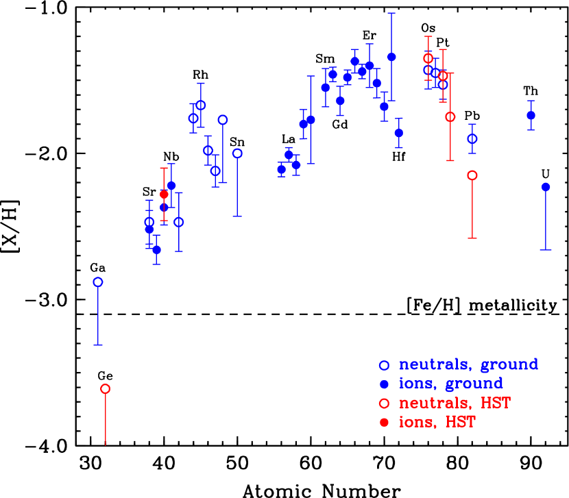
Figure 3: Abundances with respect to the Sun [X/H] versus atomic number for elements with Z $>$ 30. The symbols are defined in the figure legend, and as in Figure 1 a dashed line represents the [Fe/H] metallicity of CS 22892-052. Detected elements are shown with complete error bars, and upper limits are shown with only the lower half of an arbitrary-length error bar. A few element symbols are marked to help with identification of the points.

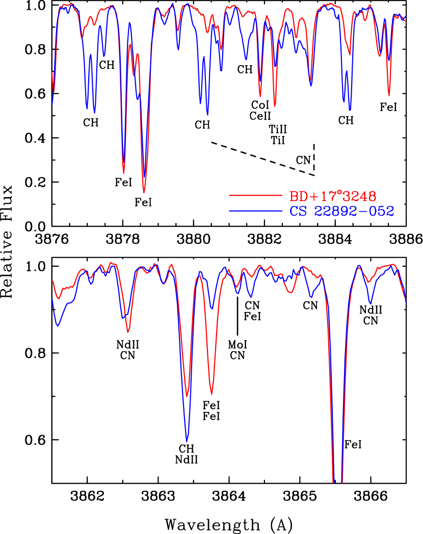
Figure 4: Spectra of CS 22892-052 and BD +17^∘3248 (Cowan et al. 2002) in two small spectral regions relevant to detection of the Mo I 3864.10 Å line. In the top panel the wavelength region near the CN $B^{\rm 2}\Sigma^{+}-X^{\rm 2}\Sigma^{+}$ (0-0) bandhead is shown, and in the bottom panel a small portion of spectrum surrounding the Mo I line is shown. A few major feature identifications are labeled in each panel, and the growth of CN strength with increasing wavelength toward the 3883.4 Å bandhead is indicated by dashed lines in the top panel.

The derived abundances of the $n$-capture elements are listed in Table 5, and their [X/H] values are displayed in Figure 3. The relation between measured $\sigma$ values and adopted error bars in this table and remaining figures for these elements follow the rules described previously for the lighter elements. The general shape of this abundance distribution, increasing [X/H] with increasing atomic number up to Z $\approx$ 65, is not new and can be compared to a similar plot in Figure 4 of Sneden et al. (1996). But the present results are based on 36 abundances or significant upper limits compared with the 20 reported by Sneden et al. The total number of transitions involved is 299 compared to the earlier 125. For species with two or more transitions, the median of the sample deviations $\sigma$ is 0.10 (Table 5) compared with 0.15 (Table 2 of Sneden et al.).

When an abundance has been determined from many lines (N $\gtrsim$ 5) its internal abundance uncertainty is small. Moreover, intercomparisons of any two $n$-capture elemental abundances derived from the same species (e.g., [Ru I/Pd I] or [La II/Eu II]) are likely to have small external errors because atmospheric parameter uncertainties produce (roughly) the same effects on both elements in the ratios. We have argued in past papers (e.g., Sneden et al. 1996) that LTE analyses should be reasonable approximations for the $n$-capture elemental abundances derived from ionized transitions. Additionally, to the extent that possible departures from LTE affect ionization equilibria in similar ways, the general agreement between abundances from neutral and ionized transitions of six Fe-peak elements (Table 4) and of Sr (Table 5) lends confidence in the general $n$-capture abundance results derived from neutral species. Statistical equilibrium computations could potentially settle such questions, but are beyond the scope of this paper. Indeed these “NLTE” studies probably are not possible for each element at present, due to the incompleteness of atomic data for many species.

Our earlier papers on CS 22892-052 have included discussions of elements with multiple detected transitions for which abundance computations are relatively straightforward. As one example, consider La. Parameters of La II lines have been taken from a recent comprehensive lab study (Lawler et al. 2001). For CS 22892-052, there are 15 lines contributing to the mean La abundance, with very small line-to-line scatter ($\sigma$ = 0.05, Table 5). We regard the La abundance as secure, and little comment is needed for this and many other elements.

In the next two subsections we will focus attention on more difficult situations: abundances and upper limits determined from one or two spectral features. These abundances cannot be employed with the same confidence as can those of “the usual suspects” among the $n$-capture elements. The cases of Mo and Sn will be used as illustrative examples to show the prospects and perils of the new element search we have conducted for CS 22892-052. In a third subsection comments will be given as needed for other $n$-capture element abundance analyses.

3.2.1 Detection of Molybdenum

In the visible and near-UV spectral regions only Mo I lines will be detectable in cool, metal-poor stars; strong Mo II lines occur only in the vacuum UV. We searched the transition probability compendium of Whaling & Brault (1988) for promising Mo I lines, and found about 10 of them that merited closer investigation. Frustratingly, all but one of these lines proved to be either undetectably weak or severely blended in our CS 22892-052 spectra. The unusable transitions include all the ones that were employed in the Biémont et al. (1983) solar Mo abundance study. The elimination process left only the 3864.10 Å line.

There is an absorption clearly visible at 3864.10 Å in the CS 22892-052 spectrum, but is it due to Mo I? The Mo contribution to this feature is very difficult to detect in most cool (T_eff $<$ 6000 K) stars, because it is intrinsically weak and is buried beneath strong CN $B^{\rm 2}\Sigma^{+}-X^{\rm 2}\Sigma^{+}$ violet system (0-0) and (1-1) band lines. Only in the relatively rare stars like CS 22892-052 can low metallicity and large departures from the Solar abundance mix potentially combine to reveal the presence of the Mo I contribution. But there are also other potential contaminants in this very crowded spectral region, including lines of the CH $B^{\rm 2}\Pi-X^{\rm 2}\Pi$ system as well as Fe-peak and $n$-capture atomic features. Disentangling all these potential contributors to the 3864.10 Å feature is another process of elimination.

To help in this effort, we compared our CS 22892-052 spectrum to that of BD +17^∘3248 (Cowan et al. 2002), an $r$-process-rich star with somewhat different characteristics than CS 22892-052. Forming differences $\delta$ in the sense BD +17^∘3248 $minus$ CS 22892-052, first note that BD +17^∘3248 is hotter ($\delta$T_eff = +400 K) and so will have intrinsically weaker spectral absorption lines for any element with equal abundances in the two stars. Second, BD +17^∘3248 is less metal-poor ($\delta$[Fe/H] = +1.0). Third, the $n$-capture abundance patterns are essentially identical in these two stars, but $\delta$[Eu/H] = +0.3 (the larger metallicity of BD +17^∘3248 wins out over the larger relative $n$-capture enhancements of CS 22892-052). Fourth, C is more abundant in CS 22892-052 ($\delta$[C/H] = –0.4), but N is slightly more abundant in BD +17^∘3248 ($\delta$[N/H] = +0.2). These differences in effective temperature and abundances lead to substantial differences in the spectra near the Mo I 3864.10 Å line.

In Figure 4 two small spectral regions of CS 22892-052 and BD +17^∘3248 are displayed. In the top panel, a 10 Å segment surrounding the CN violet system (0-0) bandhead illustrates the differences of molecular and Fe-peak line absorptions in the two stars. The CH lines of CS 22892-052 are 5-10 times stronger than in they are in BD +17^∘3248, a combined consequence of its larger C abundance and lower T_eff. The ratio of CN strengths is about a factor of three at the bandhead (the T_eff difference is the cause here, as the C+N abundances are similar in the two stars). Away from the bandhead the CN lines are very weak in both stars. The Fe-peak lines are 1.5-2 times stronger in BD +17^∘3248, due to its higher metallicity.

As shown in the bottom panel of Figure 4, the absorption in the two stars at the Mo I wavelength is nearly identical. This equality suggests which species probably are $not$ dominating the feature: CH and atomic lines of elements with Z $\leq$ 30. If the 3864.10 Å feature is caused by CH, the absorption in CS 22892-052 would be overwhelmingly larger than in BD +17^∘3248. If it is caused by a line of a “light” element, the BD +17^∘3248 spectrum should have the stronger absorption. A conspiracy between CH and atomic contaminants creating similar 3864.10 Å lines in the two stars cannot be totally ruled out, but our synthetic spectrum line list culled from the Kurucz (1995) database has no neutral and ionized lines of Z $\leq$ 30 elements within $\pm$0.09 Å of this wavelength.

As indicated in the bottom panel of Figure 4, some CN absorption should exist in the 3860-3868 Å region of the CS 22892-052 spectrum. The positive identification of CN features from our synthetic spectrum calculations is supported by the much weaker absorption at these wavelengths in the BD +17^∘3248 spectrum. Trial synthetic spectra that forced agreement with the observed features at 3864.3, 3865.2, and 3866.0 Å suggest three related points: $(a)$ the implied N abundance is $\sim$0.5 dex larger than that given in Table 4, which was derived from the 3883 Å bandhead; $(b)$ this same N abundance produces absorptions that are obviously too strong for the observed CN features in neighboring spectral regions; and $(c)$ the CN part of the 3864.10 Å feature is at most 20-30% of the total absorption.

If the absorption at 3864.1 Å is attributable to neither CH nor lighter atomic species, and has only a small CN contribution, it could be due to an $n$-capture species other than Mo I. Two possible such lines are known. First, Palmeri et al. (2000) list a Ce II line at 3864.107 Å, but the combination of its EP = 0.96 eV and log $gf$ = –2.04 render its absorption undetectably small unless the Ce abundance is a factor of $\sim$10 larger than we have derived (Table 5). Second, Kurucz (1995) lists a Sm II line at 3864.047 Å, with EP = 0.66 eV and log $gf$ = -1.15. These line parameters are more favorable, and increasing our derived Sm abundance by only 2-3 times produced detectable absorption. But this distorts the line profile to the blue by unacceptable amounts. Thus the other known $n$-capture contributors to the 3864.1 Å feature are insignificant contaminants to the Mo I line.

With attention to the above issues, we have derived log $\epsilon$(Mo) = –0.55. Tests with adding or subtracting contamination from other species suggests that the 3864.1 Å feature can be matched by Mo abundances that vary by at most 0.2 dex, yielding in particular an upper limit to the abundance of $\approx$–0.3. We attach the estimated 0.2 dex uncertainty to the Mo value in all abundance plots to follow.

3.2.2 Non-detection of Tin

A search was made for lines of Sn I in the manner described above for Mo I; strong lines of Sn II occur only in the vacuum $UV$. In the visible and near-$UV$ spectral regions, the only two that appeared to be potentially detectable and relatively unblended lie at 3262.34 and 3801.02 Å. Atomic and molecular line lists for several Å surrounding these two lines were assembled in the usual manner, and applied to our observed (Keck) spectra of CS 22892-052. Comparisons of synthetic and observed spectra are displayed in Figure 6. Neither Sn I line is clearly present in our data.

These two lines do not present ideal cases for Sn detection, as each is clearly contaminated by other absorptions. The blending agents for the 3262 Å line are Sm II 3262.27 Å and Os I 3262.29 Å; their contributions to the observed feature in the upper panel of Figure 6 are roughly equal. Repeated trial synthetic spectra demonstrated that the Sn I line cannot account for this feature, mainly because it lies 0.05 Å to the red of the observed absorption. But our synthetic spectrum in this small wavelength interval does not adequately reproduce several other observed features, which does not inspire confidence in a detailed analysis of the 3262.33 Å line. A better overall match between observed and synthetic spectra is seen in the bottom panel of Figure 6 for the 3801.02 Å line. The Sn I line is bounded to the blue mainly by Sm II 3800.89 Å and to the red by Nd II 3801.12 Å. Their absorptions are clearly present but that of Sn I is not obvious in the observed CS 22892-052 spectrum.

Our estimation that log $\epsilon$(Sn) $<$ 0.0 is strengthened from the non-detection of $both$ Sn I lines. If only one line had been available for analysis the abundance limit would probably have been higher, with larger uncertainty.

3.2.3 Other $n$-Capture Abundances

$Sr,Ba,and~{}Yb:$ The atomic structures of the ionized species of these elements produce 2-4 extremely strong resonance and low-excitation transitions (e.g., Sr II 4077.7 Å, Ba II 6141.7 Å). Analyses of these features dominate the large abundance literature for Ba and Sr. The occurrence of both Yb II resonance lines below 3700 Å has severely limited studies of this element. All of these lines lie on the flat or damping part of the curve-of-growth in the spectra of $n$-capture-rich metal-poor giants. These elements have multiple isotopes, of which the odd-mass ones have substantial hfs. Both of these effects must be carefully accounted for in synthetic spectrum computations, and still the derived abundances from such deep and saturated absorption features are dependent on assumed values of microturbulent velocity. In the present analysis, however, we have been able to detect two very weak high-excitation lines of Sr II and the weak resonance line of Sr I (Table 3). These transitions yield abundances that are consistent with the two very strong Sr II resonance lines. Abundances from three high-excitation Ba II lines agree with the results from the low-excitation features. The abundances from the strong low-excitation ionized lines appear to be reliable in CS 22892-052.

$Cd:$ Sneden et al. (2000) claimed detection of this element, and they derived log $\epsilon$(Cd) = –0.35 $\pm$ 0.20 from analysis of just the Cd I 3261.05 Å transition. We re-examined the Cd abundance, and confirmed that there are no other Cd I or Cd II lines strong enough to be useful abundance indicators in CS 22892-052. However, our new exploration of the 3261.05 Å line highlighted the possibly substantial contribution of an OH line at the same wavelength to the total absorption feature. If the OH line is neglected we derive log $\epsilon$(Cd) $\sim$ 0.0. Inclusion of the OH at a strength consistent with other probable OH lines in this spectral region suggests that it might dominate the 3261 Å contribution. Therefore we have chosen in Table 5 and in $n$-capture abundance figures to enter log $\epsilon$(Cd) $<$ 0.0. This abundance limit should be viewed with caution.

$Ge,Y,Os,Pt,Au,and~{}Pb:$ Abundances for these elements are wholly or partly determined from our HST spectrum. The general concordance of HST-based abundances of Y, Os, and Pt with those determined from ground-based data increases confidence in the HST data, even though it has relatively poor S/N. The very low abundance of Ge determined from the HST spectrum of the Ge I 3039.07 Å line gains some support from the the low Ga abundance implied from the non-detection of the Ga I 4172.04 Å feature in our Keck and VLT spectra. Finally, we are not confident of the suggested detections of two Pb I lines in the ground-based spectra. These lines should be nearly ten times weaker than the 2833.05 Å line, which we cannot detect in the HST spectrum. The derived Pb abundance upper limit from the 2833 Å line may well be more reliable than the abundances determined from the questionable detections of the other two Pb I lines.

4 DISCUSSION

4.1 Neutron-Capture Abundance Comparisons

Our new observations have provided abundances or upper limits for 36 n-capture elements, including seven more (Ga, Ge, Mo, Sn, Lu, Pt, Au) not seen in our previous study of CS 22892-052 (Sneden et al. 2000a). This provides more abundances than any other halo star, or in fact any other star except the Sun.

4.1.1 Heavier N-Capture Elements

In Figure 6 we compare these abundances in CS 22892-052 with the (scaled) solar system $r$-process abundance curve. This distribution, indicated by the solid line, is based upon $n$-capture cross section measurements (Käppeler et al. 1989; Wisshak et al. 1996) and assumes the “classical” $s$-process empirical relation between abundance and cross section. The resulting $r$-process isotopic abundances are the difference between the solar value and the individual $s$-process isotopic abundances. Summing the isotopic abundances results in the $r$-process elemental abundance distribution (Burris et al. 2000). It is clear from Figure 6 that the relative abundances of the heaviest $n$-capture elements, 56 $\leq$ Z $\leq$ 82, are all consistent with the solar system $r$-process curve. This confirms and extends the previous results in CS 22892-052 (Sneden et al. 2000) and in other stars (Westin et al. 2000; Johnson & Bolte 2001; Cowan et al. 2002; Hill et al. 2002). However, for CS 22892-052 and the majority of the other cases there was very limited data of the heaviest 3^rd $r$-process peak elements, with dominant transitions in the $UV$ necessitating HST observations. The agreement between the $n$-capture abundances in this old halo star and the solar distribution strongly supports the claim of a robust $r$-process over the history of the Galaxy, at least for the elements Ba and above.

Support for this conclusion is also found in recent isotopic abundance studies. Sneden et al. (2002) found that the ¹⁵¹Eu and ¹⁵³Eu isotopes in three halo stars, including CS 22892-052, are in agreement with each other and in solar proportions. From an analysis of another metal-poor star (HD 140283), Lambert & Allende-Prieto (2002) find that the isotopic fractions of Ba are also consistent with the solar $r$-process values.

As one further indication of the abundance history of these elements prior to the formation of CS 22892-052, we also show in Figure 6 an abundance comparison with the solar system $s$-process elemental distribution (dashed line) from Burris et al. (2000). This comparison demonstrates clearly that these elements observed in CS 22892-052, including “traditional” $s$-process elements such as Ba, were synthesized solely in the $r$-process and not in the $s$-process in a previous stellar generation early in the history of the Galaxy.

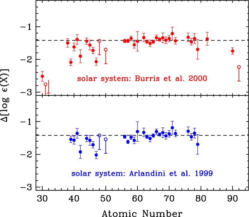
Figure 7: Differences between CS 22892-052 abundances and two scaled solar-system abundance distributions. The dotted line in each panel indicates the unweighted mean difference for elements in the range 56 $\leq$ Z $\leq$ 79. The symbols are as in Figure 6. In the top panel the abundance differences relative to those of Burris et al. (2000; their Table 5) are displayed. The upper limit for Ge (Z = 32) has no open-circle head because its upper limit lies below the lower limit boundary of the plot. In the bottom panel the abundance differences are relative to those of Arlandini et al. (1999). Their solar-system $n$-capture abundances were tabulated only for the atomic number range 39 $\leq$ Z $\leq$ 81.

A detailed element-by-element difference comparison between the solar $r$-process elemental curve from Burris et al. (2000) and the abundances in CS 22892-052 is presented in the top panel of Figure 7. The mean difference between the solar curve and the CS 22892-052 abundances (in log $\epsilon$ units) for 56 $\leq$ Z $\leq$ 79 is –1.42 $\pm$ 0.02 ($\sigma$ = 0.10; see Table 6). That is, the mean stellar abundance level of these elements is deficient with respect to the solar $r$-process abundance set by a factor of $\simeq$ 25, but enhanced with respect to the CS 22892-052 Fe abundance by a factor of $\simeq$ 45. The very small $\sigma$ is consistent with stellar and solar abundance uncertainties. In addition to the curve from Burris et al., there have been other solar r-process abundance determinations. Rather than assuming the model independent, but empirical, “classical” $s$-process relationship, more sophisticated stellar models based upon $s$-process nucleosynthesis in low-mass AGB stars have been developed to predict the isotopic $s$-process contributions to the solar abundances (Arlandini et al. 1999). In the lower panel of Figure 7 we make a similar comparison between the Arlandini et al. solar system $r$-process curve and the abundances in CS 22892-052. The mean difference and its uncertainty are nearly identical to the comparison with the Burris et al. data. This testifies to the success of the Arlandini et al. model in fitting the solar system heavy element $s$-process abundances.

While the overall agreement between the abundances in CS 22892-052 and these two solar system $r$-process curves is excellent, there are some small deviations for a few elements (e.g., Lu and Au). It might be important to examine additional cases with such deviations. In some earlier studies small differences between the elemental abundances and the solar curve were the result of inadequate atomic physics data (e.g., oscillator strengths). Most of these anomalies have been corrected by recent lab atomic data studies. We also note that for cases for which the $s$-process contributions to a solar elemental abundance completely dominate the $r$-process contributions, the uncertainties associated with the extracted $r$-process residuals can be extremely large.

4.1.2 Lighter $n$-Capture Elements

It is clear from examination of Figure 6 and Figure 7 that some of the lighter n-capture elements, those below Ba, show significant deviations from the solar $r$-process curve. Until recently there have been little data available on the lighter $n$-capture elements, particularly those in the range 41 $\leq$ Z $\leq$ 55. Abundance results for BD +17^∘3248 (Cowan et al. 2002) indicate that a few of the elements in this regime, specifically the element Ag, appear to deviate from the same solar curve that fits the heavier $n$-capture elements. This perhaps supports an earlier suggestion, based upon solar system meteoritic studies, of two $r$-processes — one for the elements A $\gtrsim$ 130-140 and a second $r$-process for the lighter elements (Wasserburg, Busso & Gallino 1996). As illustrated in Figure 6 and Figure 7, we have now detected 5 elements in this lighter element regime for CS 22892-052, and also obtained two significant abundance upper limits. Note that Ag and Mo fall well below the scaled solar $r$-process curve. The abundance of Pd also falls below the solar curve, while both Nb and Rh lie on, or very near this distribution. The upper limit on Cd (and Sn with respect to the Arlandini et al. predictions) could also be consistent with the heavier $n$-capture abundances. On average, however, these lighter elements do seem to have been synthesized at a lower abundance level than the heavier $n$-capture elements. The mean difference between the solar curve and the CS 22892-052 abundances for 38 $\leq$ Z $\leq$ 55 is –1.70 and –1.65 with a scatter $\sigma$ about the mean of 0.26 and 0.22 with respect to Burris et al. (2000) and Arlandini et al., respectively (Table 6).

There are several possible explanations for the differences in the abundance data for the lighter and heavier n-capture elements. It has been suggested for example that perhaps, analogously to the $s$-process, the lighter elements might be synthesized in a “weak” r-process with the heavier elements synthesized in a more robust “strong” (or “main”) r-process. Supernovae of a different mass range or frequency (Wasserburg & Qian 2000) or the helium zone of an exploding supernovae (Truran & Cowan 2000), have been suggested as possible second r-process sites that might be responsible for the synthesis of nuclei with A $\lesssim$ 130–140. Alternative interpretations have suggested that that the entire abundance distribution could be synthesized in a single core-collapse supernova (Sneden et al. 2000a; Cameron 2001).

We also note that the upper limits on Ga and Ge are significantly below the solar r-process curve. These elements have significant contributions from $n$-capture synthesis (Burris et al. 2000). However, the very low upper limits are more suggestive of an abundance that scales with the very low iron abundance in this star, similar to that seen in several other metal-poor halo stars (Sneden et al. 1998). Additional studies of the nature of the synthesis of Ga and Ge in other stars are currently underway (Cowan et al. 2003).

4.2 Theoretical Predictions

Our reported observations of the heavy element abundance patterns in CS 22892-052 reveal and confirm two important features that are common to extremely metal deficient stars: (1) the robustness of the goodness of fit to solar system $r$-process abundances, for elements in the range from barium to lead; and (2) the underproduction of $r$-process elements in the region of mass number below barium (A $\lesssim$ 130-140) relative to the barium-to-lead element region. We proceed now on the assumption that the robustness in the heavy region continues through the actinides, so that we can utilize abundance data concerning the interesting actinide radioactivities ²³²Th, ²³⁵U, and ²³⁸U to date the star. A potential test of this robustness follows from theoretical calculations of $r$-process synthesis. Specifically, a better understanding of both of the features identified above can be gained by comparison of representative calculations of $r$-process nucleosynthesis with the abundances determined for CS 22892-052. Note again that the large enhancement of $r$-process products relative to iron in CS 22892-052 makes this a particularly appropriate choice for this kind of analysis.

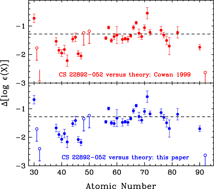
Figure 8: Differences between CS 22892-052 abundances and two scaled $r$-process theoretical predictions. The symbols and lines have the same meaning as in Figure 7. In the top panel the abundance differences relative to those of Cowan et al. (1999) are displayed. In the bottom panel the abundance differences are relative to those newly computed for this paper.

Abundance comparisons with theory are shown in Figure 8, for two specific $r$-process calculations. Both are based upon the equilibrium (i.e., “waiting point approximation”) model for the $r$-process. The first, shown in the top panel of Figure 8, was presented and discussed by Cowan et al. (1999). These calculations utilized a mass formula based upon the ETFSI-Q (Extended Thomas Fermi with Strutinski Integral and Quenching) model. The calculations consisted of a 16 component least-squares fit to the solar abundance distribution in the mass range 80 $\leq$ A $\leq$ 208. For the purpose of this paper, these calculations have now been updated and improved, with the inclusion of recent experimental determinations of half lives and neutron pairing energies (Pfeiffer, Kratz & Moeller 2002; Moeller, Pfeiffer & Kratz 2002). The calculations have then been fit to the solar $r$-process abundances in the mass range 125 $\leq$ A $\leq$ 209. Comparisons of these new theoretical results with CS 22892-052 abundances are shown in the lower panel of Figure 8.

It is clear from the comparisons summarized in both panels of Figure 8 that the agreement with $r$-process in the mass region (130 $\lesssim$ A $\lesssim$ 208) is extremely good, with a mean offset of -1.3, similar to that found for Burris et al. and Arlandini et al. (see Table 6). The scatter about the mean for the theoretical predictions is somewhat larger, when compared to the other solar comparisons, with $\sigma$ = 0.26. The theoretical comparisons again confirm a significantly lower abundance level for the lighter n-capture elements in CS 22892-052 with respect to solar r-process curve – the mean differences and $\sigma$ values very close to what was found in the Burris et al. and Arlandini et al. comparisons.

The excellent agreement between theory and observed heavy element $r$-process abundances gives us some confidence in proceeding to utilize the Th and U chronometers to provide an age estimate for CS 22892-052.

4.3 Cosmochronometry

We now employ the radioactive abundances to make cosmochronometric age estimates for this star. There have been a number of recent detections of Th in halo and globular cluster stars (Sneden et al. 1996, 2000b; Cowan et al. 1999, 2002; Westin et al. 2000; Johnson & Bolte 2001; Cayrel et al. 2001). Comparison of the observed stellar abundances of the radioactive elements and the initial abundances of these elements during $r$-process synthesis leads to a direct radioactive age determination. These chronometric age estimates, however, depend sensitively upon the predicted initial values of the radioactive elements, in ratio to each other, or to stable elements. To determine these initial ratio values we have utilized the theoretical $r$-process predictions described above in §4.2. Constrained by reproducing the observed stable element abundances observed in CS 22892-052, the earlier calculations (Cowan et al. 1999) suggested an initial value, resulting from $r$-process nucleosynthesis, of Th/Eu = 0.48. Comparing the observed Th/Eu ratio to this theoretically predicted (time-zero) Th/Eu value yields a chronometric age of 14.1 Gyr. The newer refined theoretical calculations, including more experimental values, yields an initial value of Th/Eu = 0.42, and leads to a chronometric age estimate of 11.4 Gyr. This spread in ages demonstrates the sensitivity of the radioactive dating method and provides a rough estimate of the uncertainties associated with the theoretical predictions from some of the best available $r$-process mass formulae and models. As illustrated in Figure 7, the Eu abundance value lies slightly below (by 0.04 in log $\epsilon$) the mean fit to the rare earth elements – this is a measure of the observational uncertainty, and in this case would lead to an increase in the age estimates of approximately 1.8 Gyr.

We show in Table 7 the mean age estimates for CS 22892-052, where we have taken the average predicted values from the two model calculations in comparison to the newly-determined oberved abundance values. Thus, for example, this averaging yields an age of 12.8 Gyr based upon the Th/Eu chronometer. We can also employ the abundances of some of the third $r$-process-peak elements for age estimates. Ignoring the relatively uncertain Os abundance for these estimates, averages for the chronometer pairs Th/Ir and Th/Pt suggest ages ranging from 10.5 to 19.2 Gyr (see Table 7) . An average of those values suggests an overall chronometric estimate of 14.2 $\pm$ $\simeq$ 3 Gyr. These chronometric values can be compared with our previous age estimate of 15.6 $\pm$ 4 Gyr (Sneden et al. 2000a) for this star – the differences resulting from slightly different abundance determinations and different theoretical predictions for the initial abundances.

As an additional indication of the age of this star we list in Table 7 the solar system ratios for the various chronometers. These values are measured and do not depend upon theoretical predictions and their associated nuclear physics uncertainties. Thus, we can compare the solar values (as an indication of the initial zero decay-age $r$-process abundance ratios) with the observed stellar values. However, since the Sun is only approximately 4.5 Gyr old, the solar ratios do include Galactic chemical evolution effects and represent a lower limit to the zero decay-age $r$-process abundances. This follows since Eu is stable but Th (while constantly produced and ejected into the interstellar medium) has partially decayed in the time between the formation of the oldest stars and the Sun. This leads, in general, to lower (with respect to theoretical zero decay-age $r$-process) values of Th/(stable elements) for solar ratios. Therefore, the ages derived with the solar ratios should be viewed formally as lower limits. We note, however, that there are cases where some of the predicted ages are less than the expected lower limit solar system age estimates. This is an indication that some of the theoretically predicted abundances need to be revised – for example, an overestimate of the abundance of Pt and corresponding underestimate for Ir. Such revisions are currently underway (Burles et al. 2003). Nevertheless, there is a large overlap in the lower limit age estimates with those based upon theoretical $r$-process predictions. An average of the chronometer pairs, assuming initial solar system ratios, gives an age of 14.7 Gyr, which is not inconsistent with the average based upon theoretically predicted $r$-process abundance ratios.

While Th/Eu has been utilized extensively for chronometric age estimates (Sneden et al. 1996,2000; Cowan et al. 1999, 2002; Johnson & Bolte 2001) this ratio gives a very unrealistic age estimate in CS 31082–001 (Cayrel et al. 2001; Hill et al. 2002; Schatz et al. 2002; Wanajo et al. 2002). The detection of U in that star allows for a second $r$-process chronometer and suggests an age of 14.1 $\pm$ 2.5 Gyr (Wanajo et al.) to 15.5 $\pm$ 3.2 Gyr (Schatz et al.). Since Th/Eu and Th/U give similar age results (13.8 $\pm$ 4 Gyr) for BD +17^∘3248 (Cowan et al. 2002), it is not clear yet why CS 31082–001 is so different. It does suggest that Th/U is a more reliable chronometer — particularly since they are nearer together in mass number than, for example, Th and Eu. Unfortunately we are only able to determine an upper limit on U in CS 22892-052. We can employ the chronometer ratio of Th/(upper limit of U) to determine a lower limit on the age of CS 22892-052. Recent calculations suggest a possible range of the initial Th/U value of 1.45 to 1.81 (Burles et al. 2003), leading to limiting ages for this star of 12.4 and 10.4 Gyr, respectively. This implies a conservative lower limit of 10.4 Gyr, based solely upon the abundance of Th and the upper limit on the U abundance. While these values are not definitive, they are consistent with the other age determinations employing, for example, Th/Eu. It would be extremely important for chronometric studies to eventually obtain a reliable U abundance in this star.

5 CONCLUSIONS

We have conducted an extensive new abundance analysis of the very-metal-poor, $n$-capture-rich, halo giant star CS 22892-052. We have employed high resolution spectra obtained with echelle spectrographs of HST, Keck I, McDonald, and VLT. We have obtained abundances for 52 elements and meaningful upper limits for five more elements, the largest set of elements analyzed in any star other than the Sun. New detections in CS 22892-052 include the $n$-capture elements Mo, Lu, Au, Pt and Pb, and upper limits encompass Ga, Ge, Cd, Sn, and U.

We have derived abundances for both ionization stages of six Fe-peak elements, lending confidence to the derived model atmosphere for CS 22892-052. Abundances of the volatile light elements Li and Be indicate large depletion factors ($>$10) for both elements, confirming the status of this star as an evolved, convectively mixed giant.

Close matches between observed abundances of stable heavy (Z $>$ 56) elements and two empirical scaled solar $r$-process abundance distributions re-enforces the suggested universality of the $r$-process in this element regime. In general, less satisfactory matches are seen for lighter $n$-capture elements – this may indicate the existence of two $r$-process sites or multiple $r$-process production parameters in single sites. Scaled theoretical $r$-process predictions give a reasonable fit to CS 22892-052 abundances (albeit with large element-to-element scatter), providing some encouragement that the predicted production ratios for Th/U and Th/Eu are realistic.

For Ga and Ge, two elements at the boundary between charged-particle fusion and $n$-capture synthesis modes, we derive upper limits much more consistent with the (very low) Fe-peak abundances than with the (enhanced) $n$-capture abundances. It would thus appear that, at least for this and some other old halo stars, $r$-process synthesis has not contributed significantly to these elements. We note that the $r$-process contributions to these lighter elements may have their origin, for example, in a quite different $r$-process site, in stars of longer lifetimes than those whose abundance products enriched the early Galactic halo gas.

The abundance of Th and the U upper limit, and the abundance of Th with respect to those of stable $n$-capture elements in CS 22892-052, yield self-consistent chronometric ages. This is encouraging particularly in light of the fact that this appears not to be true for the halo star CS 31082-001 (Hill et al. 2002). The detection of Th and the upper limit on the U abundance together imply a lower limit of 10.4 Gyr on the age of CS 22892-052, quite consistent with the Th/Eu age estimate of 12.8 $\pm$ $\simeq$ 3 Gyr. An average of several chronometric ratios suggests an overall chronometric age estimate of 14.2 $\pm$ $\simeq$ 3 Gyr for CS 22892-052.

Our study comes close to exhausting the element detection possibilities for CS 22892-052. Atomic physics limitations suggest that one is not likely to detect many additional elements for this star in the near future. However, higher resolution and S/N spectra may be able to turn some of the upper limits reported here into detections. Renewed attempts to detect U would be particularly useful. Very detailed abundance distributions for additional $n$-capture-rich stars will be needed to explore further the questions raised by the present study.

Appendix A NEW ELEMENTS IN THE CS 22892-052 SPECTRUM

Many laboratory studies have contributed to the $n$-capture line lists employed in the CS 22892-052 abundance analysis. We refer the the reader to our previous papers for discussions of the following species: (a) Ge I, Nb II, Pd I, La II, Ce II, Pr II, Nd II, Eu II, Gd II, Tb II, Dy II, Os I, Ir I, Pt I, Au I, and U II: Cowan et al. (2002). (b) Sr I, Sr II, Y II, Zr II, Ba II, Sm II, Er II, and Tm II: Sneden et al. (1996). (c) Os I, Pt I, and Pb I: Sneden et al. (1998). (d) Ag I: Crawford et al. (1996). Here we discuss newly detected elements and revised data for previously known transitions in CS 22892-052.

Ga I: The $gf$ value of the 4172.04 Å line is taken from the latest NIST atomic transition probability “critical compilation” (Fuhr & Wiese 2002).

Mo I: The $gf$ value of the 3863.10 Å line is taken from Whaling et al. (1984).

Ru I: The $gf$ values are taken from Wickliffe, Salih, & Lawler (1994).

Rh I: Two sources contributed the $gf$ values for this species: Kwiatkowski et al. (1982) for 3434.89 Å, and Duquette & Lawler (1985) for 3692.36 Å.

Sn I: This species has been extensively studied in the laboratory, and the $gf$ values used here are taken from the NIST compilation (Fuhr & Wiese 2002).

Yb II: Theoretical $gf$ values have been computed by Biémont et al. (1998). We renormalized these using the accurate beam-laser lifetimes of Pinnington, Rieger, & Kernahan (1997). There are seven stable isotopes of Yb to account for, ^{168,170-174,176}Yb, and only ¹⁶⁸Yb may be neglected due to its very small fractional contribution (0.13%) to the total solar Yb abundance. The odd-numbered isotopes, ^171,173Yb have significant hfs. Data for isotopic wavelength shifts and hfs were taken from Martensson-Pendrill, Gough, & Hannaford (1994)

Lu II: The $gf$ values were taken from Quinet et al. 1999, renormalized with the recent lifetime results of Fedchak et al. (2000). Hyperfine structure constants from new laboratory measurements are reported in Appendix B. These new results are in agreement with a smaller set of published hfs measurements (Brix & Kopferman 1952). There is only one stable isotope for this element, ¹⁷⁵Lu. One of the transitions employed in our Lu analysis, 3397.07 Å, was studied in the solar spectrum by Bord, Cowley, & Mirijanian (1998), who give an extensive discussion of the surrounding complex atomic and molecular spectrum.

Appendix B New Laboratory Data for Holmium and Lutetium

New laboratory measurements of transition probabilities and/or hfs constants for Ho II and Lu II were performed as part of this study of CS 22892-052. Although there is an efficiency advantage in making a large set of measurements once an experiment is operational, the need for improved laboratory data on key lines took priority here. A more comprehensive set of measurements will be published later.

The spectrum of singly ionized holmium needs attention from laboratory spectroscopists. There is evidence that available energy levels have errors of several times 0.1 cm^-1 (Worm et al. 1990). Only a very few laser calibrated transition probabilities and hfs constants have been published (Worm et al. 1990). Although radiative lifetimes for 37 levels of Ho II were measured recently using laser induced fluorescence (Den Hartog et al. 1999), these lifetimes have not yet been combined with branching fractions to determine a large set of transition probabilities. Incomplete knowledge of the energy levels has made it difficult to measure complete sets of branching ratios or branching fractions. We have measured branching ratios for four lines needed in this study of CS 22892-052. Our measurements are from spectra recorded using the 1.0 m Fourier transform spectrometer (FTS) at the U. S. National Solar Observatory. The analysis procedure is very similar to that used in recent work on La II (Lawler et al. 2001). The new Ho II branching fractions, listed in Table 8, were combined with radiative lifetimes from Den Hartog et al. to yield the Ho II log $gf$ values of Table 3. The strong blue/UV transitions listed in the table are the 6p-6s branches from each upper level. Efforts to observe and measure the weak infrared 6p-5d branches have been partially successful. Although the infrared branches have been omitted from Table 8, their approximate effect in decreasing the dominant blue/UV branching fractions has been included.

The same FTS spectra were used to extract hfs constants and improved energy levels needed in this study. The only stable isotope of Ho has mass 165 and nuclear spin 7/2. We used the ground term hfs constant reported by Worm et al. (1990) in our analysis of the FTS data. The least-square fits to partially resolved hfs patterns are most stable if either the upper or lower level constants are fixed. Our uncertainties are thus limited by the accuracy of the hfs constants from Worm et al. which are included with our results in Table 9. Our improved energy levels are accurate to $\approx$0.003 cm^-1.

A similar analysis of FTS data was used to extract the hfs constants for Lu II, which are given in Table 10. The dominant stable isotope of Lu has mass 175 and nuclear spin 7/2. In this case it is not necessary to use any published hfs data in the least-square analysis of our FTS data because we could start the analysis on lines connected to J = 0 levels. Measurements from Brix & Kopfermann (1952) are included for comparison.

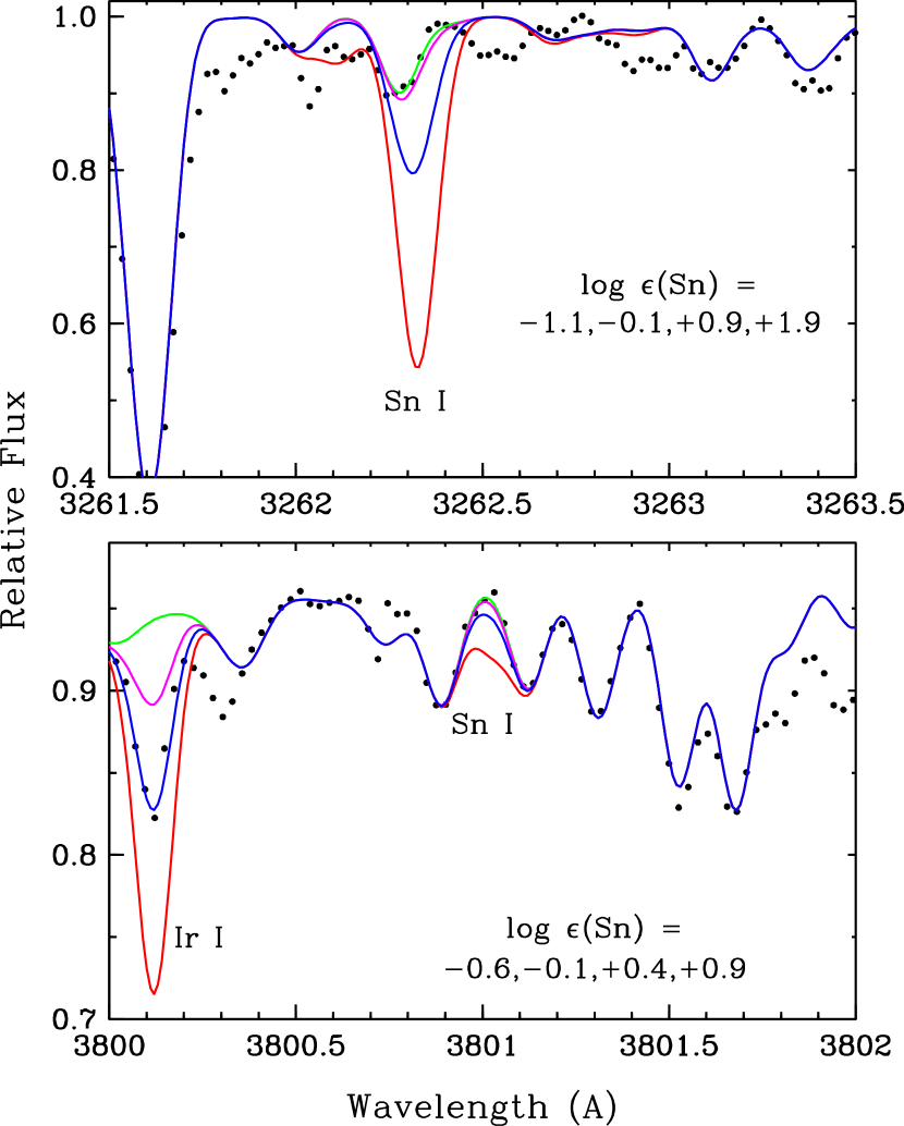
Figure 5: Observed and synthetic spectra of two Sn I lines in CS 22892-052. The assumed Sn abundances for the synthetic spectra are given in each figure panel. The synthetic spectra for two smallest abundances in each case produce nearly the same (extremely weak) Sn I absorptions. These Sn lines cannot be positively detected in CS 22892-052.

Table 1: Basic Data and Model Parameters

Quantity	Value	Source
R.A. (J2000)	$22^{h}17^{m}01.5^{s}$	1
Dec. (J2000)	$-16\arcdeg 39\arcmin 26\arcsec$	1
$l^{\rm II}$	41.15$\arcdeg$	1
$b^{\rm II}$	–52.8$\arcdeg$	1
$V$	13.18	2
$B-V$	0.78	2
$U-B$	0.14	2
$V-R$	0.48	2
$J-H$	0.47	3
$H-K$	0.11	3
$J-K$	0.58	3
$V-K$	2.26	4
$E(B-V)$	0.02, 0.00, 0.03	2,5,6
$M_{V}$	–0.23, –0.16	2,5
Distance	4700, 4648 pc	2,5
[Fe/H]C	–2.92, –3.01	2,5
Teff	4800 K	7
log $g$	1.50	7
[M/H]	–2.5	7
vt	1.95 km s-1	7

References. — 1. SIMBAD; 2. Beers et al. (1992); 3. Two Micron All Sky Survey (2MASS); 4. V from Beers et al (1992) and K from 2MASS; 5. Beers et al. (1999); 6. Schlegel et al. 1998; 7. this paper.

Table 2: Lines of Elements with Z $<$ 30 in CS 22892-052

$\lambda$	E.P.	log $gf$	E.W.	log $\epsilon$
Å	eV		mÅ
Na I, Z = 11
3302.37	0.00	–1.74	syn	+3.21
3302.98	0.00	–2.04	syn	+2.76
5889.95	0.00	+0.11	syn(150)	+3.11
5895.92	0.00	–0.19	syn(122)	+3.06
Mg I, Z = 12
3829.36	2.71	–0.21	138.0	+4.82
3832.31	2.71	+0.15	163.0	+4.82
4571.10	0.00	–5.57	30.0	+4.72
4703.00	4.35	–0.38	43.0	+4.80
5172.70	2.71	–0.38	145.0	+4.67
5183.62	2.72	–0.16	175.0	+4.90
5528.42	4.35	–0.34	44.0	+4.73
Al I, Z = 13
3961.53	0.01	–0.34	106.0	+2.79
Si I, Z = 14
4102.94	1.91	–3.10	48.0	+4.81
K I, Z = 19
7698.97	0.00	–0.17	20.0	+2.48
Ca I, Z = 20
5349.47	2.71	–0.31	5.5	+3.53
5588.76	2.53	+0.36	27.0	+3.44
5857.46	2.93	+0.24	12.0	+3.58
6102.73	1.88	–0.79	17.5	+3.58
6122.23	1.89	–0.32	38.5	+3.57
6162.18	1.90	–0.09	51.0	+3.57
6439.08	2.52	+0.39	31.5	+3.46
6493.79	2.52	–0.11	15.0	+3.54
6499.65	2.52	–0.82	3.5	+3.56
6717.69	2.71	–0.52	7.5	+3.83
Sc I, Z = 21
3911.81	0.02	+0.52	syn	–0.15:
Sc II, Z = 21
4246.83	0.32	+0.242	syn(104)	–0.18
4400.39	0.61	–0.536	syn	–0.03
5031.02	1.36	–0.400	14.0	+0.02
5526.82	1.77	+0.020	11.5	–0.05
5657.88	1.51	–0.600	6.0	–0.06
Ti I, Z = 22
3998.64	0.05	-0.06	43.0	+2.00
4533.25	0.85	0.48	22.0	+1.89
4534.78	0.84	0.28	18.0	+1.96
4548.77	0.83	-0.63	7.5	+2.43
4981.74	0.85	0.50	31.5	+2.02
4999.51	0.83	0.25	30.0	+2.21
5022.87	0.83	-0.43	7.0	+2.16
5024.85	0.82	-0.60	6.0	+2.24
5039.96	0.02	-1.13	10.0	+2.06
5064.66	0.05	-0.99	12.0	+2.04
5173.75	0.00	-1.12	10.5	+2.04
5192.98	0.02	-1.01	27.0	+2.44
5210.39	0.05	-0.88	17.0	+2.10
Ti II, Z = 22
4533.97	1.24	–0.77	87.5	+2.16
4563.77	1.22	–0.96	70.5	+1.97
4571.98	1.57	–0.53	74.5	+2.05
4589.95	1.24	–1.79	33.0	+2.16
4657.20	1.24	–2.15	10.5	+1.91
4708.67	1.24	–2.21	13.0	+2.07
5129.16	1.89	–1.39	19.5	+2.18
5154.07	1.57	–1.92	15.0	+2.19
5185.91	1.89	–1.35	12.0	+1.89
5226.55	1.57	–1.30	36.5	+2.06
5336.79	1.58	–1.70	19.0	+2.09
5381.01	1.57	–2.08	11.5	+2.20
V I, Z = 23
4111.77	0.29	+0.41	6.0	+0.71
4115.18	0.29	+0.07	3.0	+0.73
4116.47	0.28	–0.31	3.0	+1.10
V II, Z = 23
3530.76	1.07	–0.60	26.0	+0.78
3538.23	1.07	–1.64	4.0	+0.88
3545.19	1.10	–0.39	32.5	+0.75
3592.03	1.10	–0.37	42.0	+0.91
3951.97	1.48	–0.74	14.0	+0.92
4005.71	1.82	–0.46	12.0	+0.95
Cr I, Z = 24
4646.17	1.03	–0.71	17.5	+2.34
5206.04	0.94	+0.02	55.0	+2.20
5296.70	0.98	–1.40	7.0	+2.46
5345.81	1.00	–0.98	12.0	+2.32
5348.33	1.00	–1.29	8.0	+2.43
5409.80	1.03	–0.72	16.0	+2.23
Cr II, Z = 24
4588.20	4.07	–0.63	4.0	+2.33
4848.23	3.86	–1.14	3.5	+2.52
Mn I, Z = 25
4030.76	0.00	–0.47	93.5	+1.65
4033.07	0.00	–0.62	91.5	+1.74
4041.37	2.11	+0.29	18.0	+1.88
Mn II, Z = 25
3460.32	1.81	–0.54	68.0	+1.75
3488.68	1.85	–0.86	54.0	+1.84
Fe I, Z = 26
3763.80	0.99	–0.22	137.5	+4.25
3787.89	1.01	–0.84	112.0	+4.34
3820.44	0.86	+0.16	190.0	+4.29
3825.89	0.92	–0.02	179.0	+4.44
3840.45	0.99	–0.50	132.0	+4.38
3856.38	0.05	–1.28	143.0	+4.27
3865.53	1.01	–0.95	114.0	+4.45
3886.29	0.05	–1.06	187.0	+4.55
3887.06	0.92	–1.09	111.0	+4.39
3899.72	0.09	–1.52	138.5	+4.44
3917.18	0.99	–2.15	76.0	+4.58
3922.92	0.05	–1.63	137.0	+4.47
3949.96	2.18	–1.25	41.0	+4.32
4005.25	1.56	–0.58	97.0	+4.20
4071.75	1.61	–0.01	124.0	+4.31
4114.45	2.83	–1.30	11.5	+4.36
4132.91	2.85	–1.01	20.5	+4.37
4134.69	2.83	–0.65	35.5	+4.34
4143.88	1.56	–0.51	102.0	+4.18
4147.68	1.49	–2.07	51.0	+4.48
4157.79	3.42	–0.40	32.0	+4.69
4175.64	2.85	–0.83	43.0	+4.67
4187.05	2.45	–0.51	64.0	+4.31
4187.81	2.42	–0.51	81.0	+4.66
4191.44	2.47	–0.67	54.5	+4.29
4199.10	3.05	+0.16	76.5	+4.60
4202.04	1.49	–0.69	103.0	+4.28
4216.19	0.00	–3.36	79.0	+4.56
4222.22	2.45	–0.91	45.0	+4.33
4227.44	3.33	+0.27	51.0	+4.28
4233.61	2.48	–0.58	59.0	+4.29
4602.01	1.61	–3.13	8.0	+4.53
4602.95	1.49	–2.21	47.0	+4.46
4630.12	2.28	–2.59	5.0	+4.55
4647.43	2.95	–1.35	17.0	+4.68
4871.32	2.87	–0.36	51.0	+4.28
4872.14	2.88	–0.57	34.5	+4.20
4890.76	2.88	–0.39	59.0	+4.46
4891.50	2.85	–0.11	63.0	+4.22
4903.32	2.88	–0.93	25.0	+4.36
4919.00	2.87	–0.34	48.0	+4.20
4924.77	2.28	–2.20	14.5	+4.64
4938.82	2.88	–1.08	14.0	+4.19
4939.69	0.86	–3.25	26.5	+4.33
4966.09	3.33	–0.84	14.0	+4.48
4994.14	0.92	–2.97	41.0	+4.39
5001.87	3.88	+0.05	15.5	+4.27
5006.12	2.83	–0.62	40.0	+4.28
5014.94	3.94	–0.27	9.5	+4.42
5041.08	0.96	–3.09	36.0	+4.46
5049.83	2.28	–1.36	38.5	+4.34
5051.64	0.92	–2.76	59.0	+4.49
5068.77	2.94	–1.04	17.0	+4.31
5074.75	4.22	–0.16	6.5	+4.44
5079.74	0.99	–3.25	35.0	+4.64
5083.35	0.96	–2.84	42.5	+4.33
5110.44	0.00	–3.76	70.5	+4.57
5123.73	1.01	–3.06	47.0	+4.68
5125.12	4.22	–0.08	10.0	+4.56
5127.37	0.92	–3.25	30.0	+4.45
5131.48	2.22	–2.52	5.0	+4.36
5133.69	4.18	+0.20	19.0	+4.56
5141.74	2.42	–2.24	9.5	+4.61
5145.09	2.20	–2.88	4.0	+4.59
5150.85	0.99	–3.04	32.5	+4.38
5151.92	1.01	–3.32	23.5	+4.49
5162.28	4.18	+0.02	15.0	+4.61
5166.28	0.00	–4.12	41.0	+4.43
5171.61	1.49	–1.72	64.5	+4.20
5191.47	3.04	–0.55	42.0	+4.48
5192.35	3.00	–0.42	44.0	+4.34
5194.95	1.56	–2.02	51.5	+4.36
5198.71	2.22	–2.14	13.5	+4.45
5202.34	2.18	–1.84	25.0	+4.42
5216.28	1.61	–2.08	41.0	+4.30
5217.40	3.21	–1.16	9.0	+4.42
5225.53	0.11	–4.76	13.0	+4.54
5232.95	2.94	–0.06	59.5	+4.17
5247.05	0.09	–4.98	10.0	+4.60
5254.95	0.11	–4.76	11.5	+4.48
5266.56	3.00	–0.39	40.0	+4.22
5269.55	0.86	–1.33	129.0	+4.42
5281.80	3.04	–0.83	21.5	+4.33
5283.63	3.24	–0.52	27.5	+4.40
5302.31	3.28	–0.72	15.0	+4.31
5328.05	0.92	–1.47	117.0	+4.33
5328.54	1.56	–1.85	62.5	+4.36
5339.94	3.27	–0.72	19.5	+4.43
5364.87	4.45	+0.23	9.5	+4.47
5367.47	4.42	+0.44	10.5	+4.27
5369.97	4.37	+0.54	16.0	+4.34
5371.50	0.96	–1.64	110.5	+4.42
5383.38	4.31	+0.65	21.5	+4.32
5393.18	3.24	–0.72	15.0	+4.25
5397.14	0.92	–1.98	101.0	+4.48
5405.78	0.99	–1.85	96.0	+4.33
5410.91	4.47	+0.40	8.5	+4.28
5415.20	4.39	+0.64	15.0	+4.22
5424.08	4.32	+0.52	18.5	+4.37
5429.71	0.96	–1.88	103.0	+4.47
5434.53	1.01	–2.13	84.0	+4.37
5445.04	4.39	+0.04	6.0	+4.37
5446.92	0.99	–1.91	99.0	+4.44
5501.48	0.96	–3.05	42.0	+4.48
5506.79	0.99	–2.79	53.0	+4.45
5569.63	3.42	–0.50	18.0	+4.32
5572.85	3.40	–0.28	24.0	+4.24
5576.10	3.43	–0.90	11.0	+4.49
5586.77	3.37	–0.10	33.0	+4.21
5615.66	3.33	+0.05	44.0	+4.22
6065.48	2.61	–1.47	17.5	+4.31
6136.62	2.45	–1.41	30.5	+4.37
6137.70	2.59	–1.35	25.0	+4.35
6191.57	2.43	–1.42	26.0	+4.25
6213.44	2.22	–2.48	4.0	+4.15
6219.29	2.20	–2.45	9.5	+4.48
6230.74	2.56	–1.28	32.5	+4.39
6252.56	2.40	–1.77	22.0	+4.47
6265.13	2.18	–2.55	10.0	+4.59
6280.62	0.86	–4.39	7.0	+4.69
6335.33	2.20	–2.47	13.0	+4.66
6393.61	2.43	–1.57	29.5	+4.47
6400.01	3.60	–0.29	20.0	+4.34
6421.36	2.28	–2.01	13.5	+4.31
6430.85	2.18	–1.95	26.0	+4.47
6481.87	2.28	–3.01	2.5	+4.52
6494.98	2.40	–1.24	49.5	+4.45
6592.91	2.73	–1.47	17.0	+4.40
6593.87	2.44	–2.42	5.5	+4.47
6677.99	2.69	–1.42	24.5	+4.50
Fe II, Z = 26
4178.86	2.58	–2.49	34.0	+4.44
4555.89	2.83	–2.30	29.0	+4.39
4583.84	2.81	–1.89	54.5	+4.42
4923.93	2.89	–1.31	77.0	+4.31
5018.45	2.89	–1.29	78.0	+4.30
5234.63	3.22	–2.27	21.5	+4.57
5276.00	3.20	–1.96	27.0	+4.37
5284.10	2.89	–3.01	7.5	+4.40
5534.83	3.25	–2.77	6.0	+4.45
6456.39	3.90	–2.08	4.5	+4.34
6516.08	2.89	–3.45	4.5	+4.53
Co I, Z = 27
3845.47	0.92	+0.010	65.0	+1.97
3995.32	0.92	–0.220	59.5	+2.02
4121.32	0.92	–0.320	58.5	+2.07
Ni I, Z = 28
3807.15	0.42	–1.180	87.5	+3.02
3858.30	0.42	–0.970	95.5	+3.01
5035.37	3.63	+0.290	7.5	+3.09
5476.92	1.83	–0.890	40.0	+3.04
6643.64	1.68	–2.300	5.0	+3.11
6767.78	1.83	–2.170	5.5	+3.19
Cu I, Z = 29
3247.53	0.00	–0.06	syn(100)	–0.60
3273.95	0.00	–0.36	syn(76)	–0.3
Zn I, Z = 30
4810.54	4.08	–0.170	8.0	+1.69

Table 3: Lines of $n$-Capture Elements in CS 22892-052

$\lambda$	E.P.	log $gf$	EW	log $\epsilon$
Å	eV		mÅ
Ga I, Z = 31
4172.04	0.10	–0.32	syn	$<$+0.0
Ge I, Z = 32
3039.07	0.88	–0.04	syn	$<$–0.2
Sr I, Z = 38
4607.33	0.00	+0.28	syn	+0.5:
Sr II, Z = 38
3464.46	3.04	0.53	syn	+0.3:
4077.71	0.00	0.17	syn	+0.50
4161.79	2.94	–0.60	syn(6)	+0.60
4215.52	0.00	–0.17	syn(155)	+0.40
Y II, Z = 39
3242.27	0.18	+0.21	66.0	-0.35
3327.88	0.41	+0.13	55.0	-0.38
3549.01	0.13	–0.28	57.0	-0.39
3600.74	0.18	+0.28	72.0	-0.52
3611.04	0.13	+0.01	66.0	-0.48
3747.55	0.10	–0.91	32.0	-0.47
3774.33	0.13	+0.22	79.0	-0.52
3788.70	0.10	–0.07	72.0	-0.45
3818.34	0.13	–0.98	36.0	-0.30
3832.89	0.18	–0.34	60.0	-0.40
3950.36	0.10	–0.49	63.0	-0.32
4398.01	0.13	–1.00	47.0	-0.20
5087.43	1.08	–0.17	18.0	-0.59
5200.42	0.99	–0.57	11.5	-0.53
5205.73	1.03	–0.34	19.0	-0.46
Zr II, Z = 40
3054.44	0.71	–1.20	syn	+0.15
3060.11	0.04	–1.37	syn	+0.30
3061.33	0.09	–1.38	syn	+0.50
3334.62	0.56	–0.80	22.0	+0.36
3338.41	0.96	–0.58	8.5	+0.11
3410.25	0.41	–0.32	53.0	+0.42
3424.82	0.04	–1.31	21.0	+0.19
3430.53	0.47	–0.16	47.0	+0.18
3438.23	0.09	+0.42	87.0	+0.28
3457.56	0.56	–0.53	34.0	+0.34
3458.93	0.96	–0.52	9.0	+0.04
3479.02	0.53	–0.69	22.0	+0.17
3479.39	0.71	+0.17	52.0	+0.23
3499.58	0.41	–0.81	22.0	+0.14
3505.67	0.16	–0.36	53.0	+0.11
3536.94	0.36	–1.31	10.0	+0.15
3551.96	0.09	–0.31	61.0	+0.15
3573.08	0.32	–1.04	25.0	+0.32
3578.23	1.22	–0.61	4.5	+0.08
3630.02	0.36	–1.11	15.5	+0.15
3698.17	1.01	+0.09	38.0	+0.22
3714.78	0.53	–0.93	28.5	+0.46
3751.60	0.97	+0.01	33.0	+0.13
3766.82	0.41	–0.81	28.0	+0.17
3998.97	0.56	–0.67	38.0	+0.37
4050.33	0.71	–1.00	12.0	+0.20
4090.51	0.76	–1.10	12.5	+0.37
4161.21	0.71	–0.72	30.0	+0.40
4208.99	0.71	–0.46	31.5	+0.16
4317.32	0.71	–1.38	9.0	+0.39
4496.97	0.71	–0.59	26.5	+0.14
Nb II, Z = 41
3215.59	0.44	–0.19	syn	–0.90
Mo I, Z = 42
3864.10	0.00	–0.01	syn(5)	–0.40
Ru I, Z = 44
3436.74	0.15	+0.150	syn	–0.05
3498.94	0.00	+0.310	syn(19)	+0.05
3728.03	0.00	+0.270	syn	+0.1:
3798.90	0.15	–0.040	syn	+0.05
3799.35	0.00	+0.020	syn	+0.20
Rh I, Z = 45
3434.89	0.00	0.450	syn(5)	–0.60
3692.36	0.00	0.173	syn	–0.50
Pd I, Z = 46
3242.70	0.81	–0.070	syn	–0.26
3404.58	0.81	+0.320	syn(17)	–0.31
3460.75	0.81	–0.420	syn	–0.4:
3516.94	0.94	–0.240	syn(5)	–0.21
Ag I, Z = 47
3280.67	0.00	–0.04	syn(23)	–0.95
3382.90	0.00	–0.35	syn(12)	–0.80
Cd I, Z = 48
3261.05	0.00	-2.47	syn	$<$0.0
Sn I, Z = 50
3262.34	1.07	0.11	syn	$<$0.0
3801.02	1.07	0.74	syn	$<$+0.2
Ba II, Z = 56
3891.78	2.51	+0.280	syn	–0.01
4130.65	2.72	+0.560	syn	+0.04
4166.00	2.72	–0.420	syn	+0.1:
4554.03	0.00	+0.170	syn(170)	+0.07
4934.10	0.00	–0.157	syn(172)	+0.06
5853.69	0.60	–1.010	syn(65)	–0.05
6141.73	0.70	–0.077	syn(107)	–0.06
6496.91	0.60	–0.380	syn(108)	+0.06
La II, Z = 57
3713.54	0.17	–0.80	10.0	–0.86
3794.77	0.24	+0.21	45.0	–0.89
3949.10	0.40	+0.49	syn(73)	–0.88
3988.51	0.40	+0.21	syn(49)	–0.89
3995.75	0.17	–0.06	syn(46)	–0.85
4086.71	0.00	–0.07	syn(52)	–0.84
4123.22	0.32	+0.13	syn(44)	–0.89
4322.50	0.17	–0.93	12.0	–0.76
4333.75	0.17	–0.06	syn	–0.91
4526.11	0.77	–0.59	4.5	–0.87
4920.96	0.13	–0.58	25.5	–0.83
4921.78	0.24	–0.45	25.5	–0.83
5114.51	0.23	–1.03	10.5	–0.75
5797.57	0.24	–1.36	5.5	–0.77
6262.29	0.40	–1.22	4.8	–0.81
Ce II, Z = 58
3426.20	0.12	–0.62	7.5	–0.38
3539.08	0.32	–0.38	6.0	–0.51
3577.46	0.47	+0.21	15.0	–0.48
3655.84	0.32	–0.02	12.0	–0.60
3940.33	0.32	–0.27	11.5	–0.44
3942.15	0.00	–0.22	25.0	–0.46
3942.74	0.86	+0.73	17.0	–0.60
3960.91	0.32	–0.40	8.5	–0.46
3964.50	0.32	–0.54	7.0	–0.41
3984.67	0.96	+0.11	5.0	–0.46
3992.38	0.45	–0.17	7.5	–0.60
3999.24	0.30	+0.09	21.0	–0.52
4003.77	0.93	+0.30	8.5	–0.44
4014.14	0.53	+0.14	12.0	–0.59
4031.33	0.32	–0.08	12.0	–0.63
4053.50	0.00	–0.71	11.0	–0.43
4073.47	0.48	+0.23	19.5	–0.50
4083.22	0.70	+0.27	15.0	–0.42
4115.37	0.92	+0.10	5.2	–0.50
4118.14	0.70	+0.19	9.5	–0.57
4120.83	0.32	–0.21	14.0	–0.43
4127.36	0.68	+0.35	15.0	–0.53
4137.65	0.52	+0.44	28.5	–0.45
4145.00	0.70	+0.13	9.5	–0.52
4165.60	0.91	+0.53	14.5	–0.46
4539.74	0.33	–0.02	16.5	–0.59
4562.36	0.48	+0.23	25.0	–0.44
4572.28	0.68	+0.29	15.5	–0.52
4593.93	0.70	+0.11	9.0	–0.59
4628.16	0.52	+0.20	20.5	–0.48
5274.23	1.04	+0.15	7.0	–0.41
5353.52	0.88	+0.11	7.5	–0.54
Pr II, Z = 59
3964.82	0.06	+0.12	syn(18)	–1.03
3965.26	0.20	+0.14	syn(15)	–1.00
4179.40	0.20	+0.48	syn	–1.22
4189.49	0.37	+0.38	syn	–1.17
4222.95	0.06	+0.27	syn	–1.00
4408.81	0.00	+0.18	syn	–1.00
5219.05	0.79	–0.05	2.2	–1.18
5220.11	0.79	+0.30	5.2	–1.15
5259.73	0.63	+0.11	5.8	–1.11
Nd II, Z = 60
3780.40	0.47	–0.27	12.0	–0.42
3784.25	0.38	+0.23	30.0	–0.52
3784.85	0.06	–0.96	5.5	–0.60
3826.42	0.06	–0.26	20.0	–0.67
3838.98	0.00	–0.18	36.0	–0.45
3865.98	0.06	–0.80	9.0	–0.54
3866.81	0.20	–0.82	13.0	–0.17
3900.23	0.47	+0.20	23.0	–0.57
3973.30	0.63	+0.43	28.0	–0.51
4004.01	0.06	–0.59	19.0	–0.40
4013.22	0.18	–1.03	5.5	–0.43
4018.81	0.06	–0.89	14.0	–0.27
4021.34	0.32	–0.17	27.0	–0.31
4023.00	0.20	–0.19	24.5	–0.49
4041.06	0.47	–0.70	10.5	–0.11
4043.59	0.32	–0.53	9.5	–0.51
4051.15	0.38	–0.21	18.0	–0.44
4059.96	0.20	–0.33	15.0	–0.63
4061.09	0.47	+0.30	53.0	–0.09
4069.28	0.06	–0.33	26.0	–0.50
4109.45	0.32	+0.18	61.0	+0.00
4133.36	0.32	–0.52	15.0	–0.31
4211.29	0.20	–0.57	10.0	–0.62
4214.60	0.18	–1.18	3.0	–0.59
4232.20	0.06	–0.28	27.5	–0.54
4446.39	0.20	–0.63	23.5	–0.16
4462.99	0.56	–0.07	31.5	–0.11
4542.60	0.74	–0.35	11.0	–0.19
4567.61	0.20	–1.25	5.0	–0.32
4579.32	0.74	–0.55	8.0	–0.15
4594.45	0.20	–1.25	3.5	–0.48
4597.02	0.20	–0.92	13.5	–0.18
4645.77	0.56	–0.59	6.5	-0.43
4706.54	0.00	–1.50	25.0	+0.47
4715.59	0.20	–1.70	10.0	+0.44
4849.06	0.47	–0.97	10.5	+0.04
4859.02	0.32	–1.45	14.0	+0.48
4959.12	0.06	–1.37	18.0	+0.20
5092.79	0.38	–1.22	15.0	+0.33
5130.59	1.30	+0.10	8.0	–0.20
5165.14	0.68	–0.67	9.5	–0.09
5200.12	0.56	–0.50	6.5	–0.59
5212.35	0.20	–0.70	10.5	–0.60
5234.21	0.55	–0.46	12.0	–0.35
5249.60	0.98	+0.08	17.0	–0.20
5250.81	0.74	–0.56	17.5	+0.17
5255.51	0.20	–1.43	14.0	+0.27
5276.88	0.86	–0.44	5.5	–0.37
5293.17	0.82	–0.20	13.5	–0.23
5311.48	0.99	–0.56	3.5	–0.30
5319.82	0.55	–0.35	21.5	–0.17
5361.51	0.68	–0.40	8.0	–0.46
Sm II, Z = 62
3706.75	0.48	–0.63	5.5	–0.67
3760.70	0.18	–0.42	23.5	–0.52
3896.97	0.04	–0.58	17.0	–0.74
3993.30	0.04	–0.89	15.5	–0.49
4023.23	0.04	–0.83	23.0	–0.35
4068.32	0.43	–0.71	6.0	–0.68
4206.12	0.38	–1.10	6.0	–0.37
4318.94	0.28	–0.27	30.0	–0.51
4420.53	0.33	–0.38	30.0	–0.36
4519.63	0.54	–0.43	15.0	–0.46
4523.91	0.43	–0.58	12.5	–0.53
4577.69	0.25	–0.77	13.5	–0.53
4591.83	0.18	–1.21	6.5	–0.53
4642.23	0.38	–0.52	13.5	–0.63
4815.82	0.18	–0.77	10.2	–0.78
Eu II, Z = 63
3724.93	0.00	–0.09	syn	–0.95
3819.67	0.00	+0.51	syn	–0.98
3907.11	0.21	+0.17	syn	–0.97
3930.50	0.21	+0.27	syn	–0.89
3971.97	0.21	+0.27	syn	–0.99
4129.72	0.00	+0.22	syn(126)	–0.93
4205.04	0.00	+0.21	syn	–0.93
6645.04	1.38	+0.12	syn(8)	–0.98
Gd II, Z = 64
3331.40	0.00	–0.14	33.5	–0.43
3424.59	0.35	–0.17	14.0	–0.56
3439.23	0.38	+0.15	27.0	–0.46
3451.23	0.38	–0.05	16.0	–0.58
3454.90	0.03	–0.48	19.0	–0.47
3481.80	0.49	+0.23	19.0	–0.64
3549.37	0.24	+0.26	40.0	–0.48
3557.05	0.60	+0.21	15.0	–0.64
3697.75	0.03	–0.28	24.5	–0.63
3712.72	0.38	+0.15	27.0	–0.59
3768.40	0.08	+0.36	51.0	–0.66
3796.39	0.03	+0.14	54.0	–0.45
3844.58	0.14	–0.40	23.0	–0.45
3973.98	0.60	–0.40	6.5	–0.57
4037.33	0.66	–0.02	19.0	–0.36
4037.91	0.56	–0.23	11.0	–0.55
4085.57	0.73	+0.07	12.0	–0.61
4098.90	0.60	–0.45	8.5	–0.42
4191.08	0.43	–0.57	10.0	–0.44
4215.02	0.43	–0.58	12.5	–0.33
Tb II, Z = 65
3472.80	0.13	–0.10	syn	–1.09
3568.51	0.00	+0.36	syn	–1.17
3600.41	0.64	+0.60	syn(11)	–1.07
3658.89	0.13	–0.01	syn	–1.14
3702.85	0.13	+0.44	syn(21)	–1.17
3848.73	0.00	+0.28	syn	–1.14
3874.17	0.00	+0.27	syn	–1.11
Dy II, Z = 66
3407.80	0.00	+0.18	63.0	–0.20
3434.37	0.00	–0.45	40.0	–0.21
3445.57	0.00	–0.15	56.0	–0.10
3449.89	0.54	–0.75	6.5	–0.34
3454.32	0.00	–0.14	48.0	–0.34
3460.97	0.00	–0.07	54.0	–0.25
3473.70	0.93	–0.46	7.5	–0.10
3506.81	0.10	–0.60	29.0	–0.22
3531.71	0.00	+0.77	87.0	–0.14
3536.02	0.54	+0.53	47.0	–0.42
3538.52	0.00	–0.02	60.0	–0.19
3546.83	0.10	–0.55	31.0	–0.24
3550.22	0.59	+0.27	36.0	–0.35
3559.30	1.22	–0.28	6.0	–0.07
3563.15	0.10	–0.36	41.0	–0.20
3640.25	0.59	–0.37	18.5	–0.18
3694.81	0.10	–0.11	55.0	–0.24
3708.22	0.59	–0.88	6.0	–0.29
3747.82	0.10	–0.81	22.0	–0.29
3788.44	0.10	–0.57	33.0	–0.29
3983.65	0.54	–0.31	23.0	–0.29
3996.69	0.59	–0.26	24.0	–0.26
4073.12	0.54	–0.32	27.0	–0.21
4077.96	0.10	–0.04	65.0	–0.22
4103.30	0.10	–0.38	53.0	–0.15
4468.14	0.10	–1.67	5.5	–0.26
5169.69	0.10	–1.95	3.5	–0.27
Ho II, Z = 67
3810.74	0.00	+0.19	syn(80)	–0.87
3905.63	0.08	-0.53	syn	–1.0:
4045.47	0.00	-0.05	syn	–0.92
4152.58	0.08	-0.93	syn	–0.93
Er II, Z = 68
3332.70	0.89	+0.05	10.5	–0.56
3499.10	0.05	+0.14	59.5	–0.37
3559.90	0.00	–0.74	28.0	–0.34
3692.65	0.05	+0.14	63.0	–0.46
3729.52	0.00	–0.50	33.0	–0.56
3938.63	0.00	–0.52	37.5	–0.50
Tm II, Z = 69
3462.20	0.00	+0.03	syn(24)	–1.34
3700.26	0.03	–0.38	syn(17)	–1.32
3701.36	0.00	–0.54	syn(11)	–1.45
3761.91	0.00	–0.43	syn	–1.32
3795.76	0.03	–0.23	syn(21)	–1.37
3848.02	0.00	–0.14	syn	–1.39
Yb II, Z = 70
3289.37	0.00	+0.02	syn(107)	–0.57
3694.19	0.00	–0.30	syn(120)	–0.62
Lu II, Z = 71
3397.07	1.46	–0.19	syn	–1.1:
3472.48	1.54	–0.19	syn	–1.3:
3554.42	2.15	+0.14	syn	–1.1:
Hf II, Z = 72
3719.28	0.61	–0.89	syn(6)	–0.90
3793.38	0.38	–0.95	syn	–1.05
Os I, Z = 76
3058.66	0.00	–0.43	syn(30)	+0.10
3267.95	0.00	–1.08	syn(4)	–0.10
3301.57	0.00	–0.75	syn	+0.02
3528.60	0.00	–1.70	syn	+0.15
Ir I, Z = 77
3513.65	0.00	–1.26	syn	–0.05
3558.99	0.72	–1.65	syn	$<$+0.3
3800.12	0.00	–1.45	syn(11)	–0.15
Pt I, Z = 78
2929.82	0.00	–0.80	syn(44)	+0.45
2997.96	0.10	–0.57	syn	+0.2:
3301.87	0.81	–0.77	syn(13)	+0.33
3315.04	0.00	–2.58	syn	+0.2:
Au I, Z = 79
2675.94	0.00	–0.46	syn	–0.9:
Pb I, Z = 82
2833.05	0.00	-0.68	syn	$<$–0.2
3683.46	0.97	-0.60	syn	+0.1:
4057.81	1.32	-0.17	syn	0.0:
Th II, Z = 90
4019.12	0.00	-0.27	syn	–1.60
4086.52	0.00	-0.89	syn	–1.5:
U II, Z = 92
3859.57	0.04	-0.17	syn	$<$–2.3

Table 4: Abundances for Lighter Elements

Species	Z	log $\epsilon$	$\sigma$	ebar	Nlines	log $\epsilon_{\sun}$	[X/H]	[X/Fe]
Li I	3	+0.15	$\cdots$	0.30	1	$\cdots$	$\cdots$	$\cdots$
Be I	4	–2.4:	0.30	0.30	2	$\cdots$	$\cdots$	$\cdots$
CH	6	+6.30		0.10	1	8.52	–2.22	+0.88
CN	7	+5.83		0.20	1	7.92	–2.09	+1.01
[O I]	8	+6.45	$\cdots$	0.15	1	8.83	–2.38	+0.72
Na I	11	+3.04	0.19	0.19	4	6.33	–3.29	–0.19
Mg I	12	+4.78	0.08	0.08	7	7.58	–2.87	+0.30
Al I	13	+2.79	$\cdots$	0.15	1	6.47	–3.68	–0.58
Si I	14	+4.81	$\cdots$	0.15	1	7.55	–2.74	+0.36
K I	19	+2.48	$\cdots$	0.15	1	5.12	–2.64	+0.46
Ca I	20	+3.56	0.10	0.10	10	6.36	–2.80	+0.30
Sc I	21	–0.15	$\cdots$	0.15	1	3.17	–3.32	–0.22
Sc II	21	–0.03	0.04	0.05	3	3.17	–3.20	–0.10
Ti I	22	+2.12	0.17	0.17	13	5.02	–2.90	+0.20
Ti II	22	+2.08	0.11	0.11	12	5.02	–2.94	+0.16
V I	23	+0.85	0.22	0.22	3	4.00	–3.15	–0.05
V II	23	+0.87	0.08	0.08	6	4.00	–3.13	–0.03
Cr I	24	+2.33	0.11	0.11	6	5.67	–3.34	–0.24
Cr II	24	+2.42	0.14	0.14	2	5.67	–3.25	–0.15
Mn I	25	+1.76	0.12	0.12	3	5.39	–3.63	–0.53
Mn II	25	+1.80	0.06	0.15	2	5.39	–3.59	–0.49
Fe I	26	+4.40	0.13	0.13	132	7.50	–3.10	0.00
Fe II	26	+4.41	0.08	0.08	11	7.50	–3.09	+0.01
Co I	27	+2.02	0.05	0.05	3	4.92	–2.90	+0.20
Ni I	28	+3.08	0.07	0.07	6	6.25	–3.17	–0.07
Cu I	29	+0.45	0.21	0.21	2	4.21	–3.76	–0.66
Zn I	30	+1.59	$\cdots$	0.15	1	4.60	–3.01	+0.09

Table 5: Abundances for Neutron-Capture Elements

Species	Z	log $\epsilon$	$\sigma$	ebar	Nlines	log $\epsilon_{\sun}$	[X/H]	[X/Fe]
Ga I	31	$<$0.0	$\cdots$	$\cdots$	1	2.88	$<$–2.9	$<$+0.2
Ge I (HST)	32	$<$–0.2	$\cdots$	$\cdots$	1	3.41	$<$–3.6	$<$–0.5
Sr I	38	+0.50	$\cdots$	0.15	1	2.97	–2.47	+0.63
Sr II	38	+0.45	0.13	0.13	4	2.97	–2.52	+0.58
Y II	39	–0.42	0.10	0.10	15	2.24	–2.66	+0.44
Zr II	40	+0.23	0.12	0.12	28	2.60	–2.37	+0.73
Zr II (HST)	40	+0.32	0.18	0.18	3	2.60	–2.28	+0.82
Nb II	41	–0.80	$\cdots$	0.15	1	1.42	–2.22	+0.88
Mo I	42	–0.40	$\cdots$	0.20	1	1.92	–2.32	+0.78
Ru I	44	+0.08	0.10	0.10	5	1.84	–1.76	+1.34
Rh I	45	–0.55	0.15	0.15	2	1.12	–1.67	+1.43
Pd I	46	–0.29	0.10	0.10	4	1.69	–1.98	+1.12
Ag I	47	–0.88	0.11	0.11	2	1.24	–2.12	+0.98
Cd I	48	$<$0.0	$\cdots$	$\cdots$	1	1.77	$<$–1.8	$<$+1.3
Sn I	50	$<$0.0	$\cdots$	$\cdots$	2	2.00	$<$–2.0	$<$+1.1
Ba II	56	+0.02	0.05	0.05	8	2.13	–2.11	+0.99
La II	57	–0.84	0.05	0.05	15	1.17	–2.01	+3.09
Ce II	58	–0.50	0.07	0.07	32	1.58	–2.08	+1.02
Pr II	59	–1.09	0.10	0.10	9	0.71	–1.80	+1.30
Nd II	60	–0.27	0.30	0.30	52	1.50	–1.77	+1.33
Sm II	62	–0.54	0.13	0.13	15	1.01	–1.55	+1.55
Eu II	63	–0.95	0.03	0.05	8	0.51	–1.46	+1.64
Gd II	64	–0.52	0.10	0.10	20	1.12	–1.64	+1.46
Tb II	65	–1.13	0.04	0.05	7	0.35	–1.48	+1.62
Dy II	66	–0.23	0.08	0.08	27	1.14	–1.37	+1.73
Ho II	67	–0.93	0.05	0.05	4	0.51	–1.44	+1.66
Er II	68	–0.47	0.15	0.15	8	0.93	–1.40	+1.70
Tm II	69	–1.37	0.10	0.10	6	0.15	–1.52	+1.58
Yb II	70	–0.60	0.04	0.10	2	1.08	–1.68	+1.42
Lu II	71	–1.17	0.10	0.30	2	0.06	–1.45	+1.87
Hf II	72	–0.98	0.10	0.10	2	0.88	–1.86	+1.24
Os I	76	+0.02	0.13	0.13	3	1.45	–1.43	+1.67
Os I (HST)	76	+0.10	$\cdots$	0.15	1	1.45	–1.35	+1.65
Ir I	77	–0.10	0.10	0.10	2	1.35	–1.45	+1.65
Pt I	78	+0.27	0.09	0.10	2	1.80	–1.53	+1.57
Pt I (HST)	78	+0.33	0.18	0.18	2	1.80	–1.47	+1.63
Au I (HST)	79	–0.90	$\cdots$	0.30	1	0.85	–2.25	+0.85
Pb I	82	+0.05	0.07	0.15	2	1.95	–1.90	+1.20
Pb I (HST)	82	$<$–0.2	$\cdots$	0.15	1	1.95	$<$–2.2	$<$+0.9
Th II	90	–1.57	0.10	0.10	2	0.17	–1.74	+1.36
U II	92	$<$–2.3	$\cdots$	$\cdots$	1	–0.07	$<$–2.2	$<$+0.9

Table 6: Model Fits to the Data

Model	Mean Difference	$\sigma$	Model	Mean Difference	$\sigma$
	(light)	(light)		(heavy)	(heavy)
Burris et al.	-1.70 $\pm$ 0.09	0.26	Burris et al.	-1.42 $\pm$ 0.02	0.10
Arlandini et al.	-1.65 $\pm$ 0.08	0.22	Arlandini et al.	-1.42 $\pm$ 0.03	0.12
Old Theory	-1.80 $\pm$ 0.09	0.28	Old Theory	-1.28 $\pm$ 0.06	0.26
New Theory	-1.88 $\pm$ 0.09	0.28	New Theory	-1.28 $\pm$ 0.06	0.26

Table 7: Chronometric Age Estimates for CS 22892–052

Chronometer Pair	Predicted	Observed	Average Age	Solar	Lower Limit
			(Gyr)		(Gyr)
Th/Eu	0.45	0.24	12.8	0.4615	13.2
Th/Ir	0.0876	0.0339	19.2	0.0646	13.1
Th/Pt	0.0226	0.0135	10.5	0.0323	17.7
Th/U	1.45–1.805	$\geq$ 5.4	$\geq$ 10.4	—	—

Table 8: Branching Fractions for Ho II

Transition	$\lambda$	Eupper	Jupper	Elower	Jlower	Branching
cm-1	nm	cm-1		cm-1		Ratio
26234.36	381.071	26234.36	7	0.00	8	0.805$\pm$3%
25596.61	390.566	26234.36	7	637.75	7	0.145$\pm$3%
24712.16	404.545	24712.16	7	0.00	8	0.845$\pm$3%
24074.41	415.262	24712.16	7	637.75	7	0.105$\pm$3%

Table 9: Improved Energy Levels and Hyperfine Structure Constants for Ho II

Configuration	Term	J	E	A	B
			cm-1	mK	mK
${\rm 4f^{11}(^{4}I_{15/2})6s_{1/2}}$	(15/2,1/2)o	8	0.000	+52.64$\pm$0.07	–52.6$\pm$3.3
${\rm 4f^{11}(^{4}I_{15/2})6s_{1/2}}$	(15/2,1/2)o	7	637.754	+0.83$\pm$0.07	–56.4$\pm$3.5
$\cdots$	$\cdots$	7	24712.163	+42.15$\pm$0.05	+0.2$\pm$2.0
${\rm 4f^{11}(^{4}I_{15/2})6p_{1/2}}$	(15/2,1/2)	7	26234.363	+41.60$\pm$0.05	+21.6$\pm$2.0

Table 10: Hyperfine Structure Constants for Lu II

Configuration	Term	J	E	A	B	A	B
			cm-1	mK	mK	mK	mK
5d6s	3D	1	11796.24	–68.32$\pm$0.07	+29.3$\pm$0.7	–68.2	+29.0
5d6s	3D	2	12435.32	+64.39$\pm$0.10	+45.8$\pm$1.0	+64.5	+46.4
5d6s	3D	3	14199.08	+57.06$\pm$0.20	+79.2$\pm$2.0	+56.8	+76.8
5d6s	1D	2	17332.58	–25.71$\pm$0.20	+74.7$\pm$2.0	$\cdots$	$\cdots$
5d6p	3Po	1	28503.16	+165.38$\pm$0.07	–61.1$\pm$0.7	+165.4	–62.5
5d6p	3Po	2	32452.26	+95.60$\pm$0.10	+115.4$\pm$1.5	+95.9	+113.6
5d6p	3Fo	2	41224.96	+26.95$\pm$0.10	+63.9$\pm$1.0	$\cdots$	$\cdots$
5d6p	3Fo	3	44918.68	+10.90$\pm$0.20	+105.2$\pm$2.0	$\cdots$	$\cdots$
5d6p	3Fo	4	48536.83	+2.9$\pm$0.3	+192$\pm$4	$\cdots$	$\cdots$
5d6p	1Do	2	45458.56	+2$\pm$1	–10$\pm$5	$\cdots$	$\cdots$

References

- (1) Allende Prieto, C., Lambert, D. L., & Asplund, M. 2001, ApJ, 556, L63
- (2) Allende Prieto, C., Lambert, D. L., & Asplund, M. 2002, ApJ, 573, L137
- (3) Alonso, A., Arribas, S., & Martinez-Roger, C. 1999, A&AS, 140, 261
- (4) Alonso, A., Arribas, S., & Martinez-Roger, C. 2001, A&A, 376, 1039
- Arlandini et al. (1999) Arlandini, C., Käppeler, F., Wisshak, K., Gallino, R., Lugaro, M., Busso, M., & Staniero, O. 1999, ApJ, 525, 886
- (6) Barlow, T. A. & Sargent, W. L. W. 1997, AJ, 113, 136
- (7) Beers, T. C., Preston, G. W., & Shectman, S. A. 1985, AJ, 90, 2089
- (8) Beers, T. C., Preston, G. W., & Shectman, S. A. 1992, AJ, 103 1987
- (9) Beers, T. C., Rossi, S., Norris, J. E., Ryan, S. G., & Shefler, T. 1999, AJ, 117, 981
- (10) Biémont, E., Dutrieux, J.-F., Martin, I., & Quinet, P. 1998, J. Phys. B, 31, 3321
- (11) Biémont, E., Grevesse, N., Hannaford, P., Lowe, R. M., & Whaling, W. 1983, A&A, 275, 889
- (12) Blake, L. A. J., Ryan, S. G., Norris, J. E., & Beers, T. C. 2001, Nucl. Phys. A., 688, 502
- (13) Boesgaard, A. M., Deliyannis, C. P., King, J. R., Ryan, S. G., Vogt, S. S., & Beers, T. C. 1999, AJ, 117, 1549
- (14) Boesgaard, A. M., Deliyannis, C. P., King, J. R., & Stephens, A. 2001, ApJ, 553, 754
- (15) Bord, D. J., Cowley, C. R., & Mirijanian, D. 1998, Sol. Phys., 178, 221
- (16) Brix & Kopfermann 1952, in Landolt-Borstein (ed.) Zahlenwerte und Funktionen 6th Ed., Vol I, part 5 (Berlin: Springer Verlag)
- Burles et al. (2003) Burles, S., Truran, J. W., Cowan, J. J., Sneden, C., Kratz, K.-L, & Pfeiffer, B. 2003, in preparation
- (18) Burris, D. L., Pilachowski, C. A., Armandroff, T. A., Sneden, C., Cowan, J. J., & Roe, H. 2000, ApJ, 544, 302
- (19) Busso, M., Gallino, R., & Wasserburg, G. J. 1999, ARA&A, 37, 239
- (20) Cameron, A. G. W. 2001, ApJ, 562, 456
- (21) Castelli, F., Gratton, R. G., & Kurucz, R. L. 1997, A&A, 318, 841
- (22) Cayrel, R. 1996, A&A Rev., 7, 217
- Cayrel et al. (2001) Cayrel, R., et al. 2001, Nature, 409, 691
- (24) Cowan, J. J., Burris, D. L., Sneden, C., McWilliam, A., & Preston, G. W. 1995, ApJ, 439, L51
- (25) Cowan, J. J., McWilliam, A., Sneden, C., & Burris, D. L. 1997, ApJ, 480, 246
- (26) Cowan, J. J., Pfeiffer, B., Kratz, K.-L., Thielemann, F.-K., Sneden, C., Burles, S., Tytler, D., & Beers, T. C. 1999, ApJ, 521, 194
- (27) Cowan, J. J., et al. 2002, ApJ, 572, 861
- (28) Cowan, J. J., et al. 2003, ApJ, in preparation
- (29) Cowley, C. R., Ryabchikova, T., Kupka, F., Bord, D. J., Mathys, G., & Bidelman, W. P. 2000, MNRAS, 317, 299
- (30) Crawford, J. L., Sneden, C., King, J. R., Boesgaard, A. M., & Deliyannis, C. P. 1998, AJ, 116, 2489
- (31) Dekker, H., D’Odorico, S., Kaufer, A., Delabre, & B., Kotzlowski, H. 2000, in Optical and IR Telescope Instrumentation and Detectors, ed. M. Iye and A. F. Moorwood, Proc. SPIE, 4008, 534
- (32) Den Hartog, E. A., Wiese, L. M., & Lawler, J. E. 1999, J. Opt. Soc. Am. B, 16, 2278
- (33) Depagne, E. et al. 2002, A&A, 390, 187
- (34) Duquette, D. W., & Lawler, J. E. 1985, J. Opt. Soc. Am., 2, 1948
- (35) Fedchak, J. A., Den Hartog, E. A., Lawler, J. E., Palmeri, P., Quinet, P., & Biémont, E. 2000, ApJ, 542, 1109
- (36) Fitzpatrick, M. J. & Sneden, C. 1987, BAAS, 19, 1129
- (37) Fuhr, J. R., & Wiese, W. L. 2002, NIST Atomic Transition Probability Tables, in CRC Handbook of Chemistry and Physics, 83st Edition, ed. D. R. Lide (Boca Raton: CRC Press), p -88
- (38) Gilroy, K. K., Sneden, C., Pilachowski, C. A., & Cowan, J. J. 1988, ApJ, 327, 298
- (39) Gratton, R., & Sneden, C. 1994, A&A, 287, 927
- (40) Gratton, R. G., Sneden, C., Carretta, E., & Bragaglia, A. 2000, A&A, 354, 169
- (41) Grevesse, N., & Sauval, A. J., 1998, Sp. Sci. Rev., 85, 161
- (42) Hill, V. et al. 2002, A&A, 387, 560
- (43) Howeger, H. 2001, in AIP Conf. Proc. 598, Solar and Galactic Composition: A Joint SOHO/ACE Workshop, ed. R. F. Wimmer-Schweingruber (New York: AIP), 23
- (44) Johnson, J. A., & Bolte, M. 2001, ApJ, 554, 888
- (45) Käppeler, F., Beer, H., & Wisshak, K. 1989, Rep. Prog. Phys., 52, 945
- (46) Kurucz, R. L. 1995, in Workshop on Laboratory and astronomical high resolution spectra, ASP Conference Ser. #81 ed. A.J. Sauval, R. Blomme, and N. Grevesse (San Francisco: Astr. Soc. Pac.), p.583
- (47) Kwiatkowski, M., Zimmermann, P., Biemont, E., & Grevesse N. 1982, A&A, 112, 337
- (48) Lambert, D. L., & Allende Prieto, C. 2002, MNRAS, 335, 325
- (49) Lawler, J. E., Bonvallet, G., & Sneden, C. 2001, ApJ, 556, 452
- (50) Martensson-Pendrill, A-M, Gough, D. S., & Hannaford P. 1994, Phys. Rev. A, 49, 3351
- (51) McWilliam, A. 1998, AJ, 115, 1640
- (52) McWilliam, A., Preston, G. W., Sneden, C., & Searle, L. 1995, AJ, 109, 2757
- (53) Mishenina, T. V., Kovtyukh, V. V., Soubiran, C., Travaglio, C., & Busso, M. 2002, A&A, 396, 189
- (54) Moeller, P., Pfeiffer, B. & Kratz, K.-L. 2002, Phys. Rev. C, submited
- (55) Norris, J. E., Ryan, S. G., & Beers, T. C., 1997, ApJ, 488, 350
- (56) Norris, J. E., Ryan, S. G., & Beers, T. C., 1997, ApJ, 489, L169
- (57) Palmeri, P., Quinet, P., Wyart, J.-F., & Biémont, E., 2000, Phys. Scr., 61, 323
- (58) Peterson, R. C., Dorman, B., & Rood, R. T. 2001, ApJ, 559, 372
- (59) Pfeiffer, B., Kratz, K.-L. & Moeller, P. 2002, Progr. Nucl. Energ. 41, 39
- (60) Pinnington, E. H., Rieger, G., & Kernahan, J. A. 1997, Phys. Rev. A, 56, 2421
- (61) Primas, F., Asplund, M., Nissen, P. E., Hill, V. 2000, A&A, 364, L42
- (62) Primas, F., Duncan, D. K., Pinsonneault, M. H., Deliyannis, C. P., & Thorburn, J. A. 1997, ApJ, 480, 784
- (63) Primas, F., Molaro, P., Bonifacio, P., Hill, V. 2000, A&A, 362, 666
- (64) Primas, F., Reimers, D., Wisotzki, L., Reetz, J., Gehren, T., & Beers, T. C. 2000, in The First Stars, ed. A. Weiss, T. Abel, & V. Hill (Berlin: Springer), 51
- (65) Quinet, P., Palmeri, P., Biémont, E., McCurdy, M. M., Rieger, G., Pinnington, E. H., Wickliffe, M. E., & Lawler, J. E. 1999, MNRAS, 307, 934
- (66) Reetz, J. 1999, Ap&SS, 265, 171
- (67) Reyniers, M., Van Winckel, H., Biémont, E., & Quinet, P. 2002, A&A, 395, L35
- (68) Ryan, S. G., & Deliyannis, C. P. 1998, ApJ, 500, 398
- (69) Ryan, S. G., Kajino, T., Beers, T. C., Suzuki, T. K., Romano, D., Matteucci, F., & Rosolankova, K. 1999, ApJ, 549, 55
- (70) Ryan, S. G., Norris, J. E., & Beers, T. C. 1996, ApJ, 471, 254
- (71) Schatz, H., Toenjes, R., Pfeiffer, B., Beers, T. C., Cowan, J. J.; Hill, V., & Kratz, K.-L. 2002, ApJ, 579, 626
- (72) Schlegel, D. J., Finkbeiner, D. P., & Davis, M. 1998, ApJ, 500, 525
- (73) Sneden, C. 1973, ApJ, 184, 839
- (74) Sneden, C., Cowan, J. J., Burris, D. L., & Truran, J. W. 1998, ApJ, 496, 235
- (75) Sneden, C., Cowan, J.J., Ivans, I. I., Fuller, G. M., Burles, S., Beers, T. C., & Lawler, J. E. 2000a, ApJ, 533, L139.
- (76) Sneden, C., Johnson, J., Kraft, R. P., Smith, G. H., Cowan, J. J., & Bolte, M. S. 2000b, ApJ, 536, L85
- (77) Sneden, C., McWilliam, A., Preston, G. W., Cowan, J. J., Burris, D. L., & Armosky, B. J. 1996, ApJ, 467, 819
- (78) Sneden, C., & Parthasarathy, M. 1983, ApJ, 267, 757
- (79) Sneden, C., & Pilachowski, C. A. 1985, ApJ, 288, L55
- (80) Sneden, C., Preston, G. W., McWilliam, A., & Searle, L. 1994, ApJ, 431, L27
- Spite & Spite (1978) Spite, M., & Spite, F. 1978, A&A, 67, 23
- (82) Takeda, Y., Zhao, G., Chen, Y.-Q., Qiu, H.-M., & Takada-Hidai, M. 2002, PASJ, 54, 275
- Truran (1981) Truran, J. W. 1981, A&A, 97, 391
- (84) Truran, J. W., & Cowan, J. J. 2000, in Nuclear Astrophysics, ed. W. Hillebrandt & E. Müller (Munich: MPI), 64
- (85) Tull, R. G., MacQueen, P. J., Sneden, C., & Lambert, D. L. 1995, PASP, 107, 251
- (86) Vogt, S. S. et al. 1994, in Proc. SPIE Conf. 2198, Instrumentation in Astronomy VII, eds. D. L. Crawford and E. R. Craine, (Bellingham, WA: SPIE), p. 362.
- (87) Wahlgren, G. M. 2002, Phys. Scr, T100, 22
- (88) Wanajo, S., Itoh, N., Ishimaru, Y., Nozawa, S., & Beers, T. C. 2002, ApJ, 577, 853
- (89) Warmels, R.H. 1991, in Astronomical Data Analysis Software and Systems I , PASP Conf. Ser., 25, 115
- (90) Wasserburg, G. J., Busso, M., & Gallino, R. 1996, ApJ, 466, L109
- (91) Wasserburg, G. J., & Qian, Y.-Z. 2000, ApJ, 529, L21
- (92) Westin, J., Sneden, C., Gustafsson, B., & Cowan, J.J. 2000, ApJ, 530, 783
- (93) Whaling, W., & Brault, J. W. 1988, Phys. Scr, 38, 707
- (94) Whaling, W., Hannaford, P., Lowe, R. M., Bíemont, E., & Grevesse N. 1984, J. Quant. Spect. Rad. Trans. 32, 69
- (95) Wickliffe, M. E., Salih, S., & Lawler, J. E. 1994, J. Quant. Spec. Rad. Trans., 51, 545
- (96) Wisshak, K., Voss, F., & Käppeler, F. 1996, in Proceedings of the 8th Workshop on Nuclear Astrophysics, ed. W. Hillebrandt, & E. Müller ( Munich: MPI), 16
- (97) Worm, T., Shi, P., & Poulsen, O. 1990, Phys. Scr, 42, 569