Abstract

The generalized Chaplygin gas (GCG) model explains the recent accelerated expansion of the Universe via an exotic background fluid whose equation of state is given by $p=-A/\rho^{\alpha}$, where $A$ is a positive constant and $0<\alpha\leq 1$. The model is an interesting alternative to scenarios involving scalar field potentials, with the ensuing unnatural fine tuning conditions for the underlying particle physics theories. We derive constraints on the parameter space of the model from bounds on the location of the first few peaks and troughs of the the Cosmic Microwave Background Radiation (CMBR) power spectrum arising from recent WMAP and BOOMERanG data.

PACS number(s): 98.80.Cq

1 Introduction

It has recently been proposed that the evidence for a dark energy component to the total energy density of the Universe at present might be explained by a change in the equation of state of the background fluid rather than by a cosmological constant or the dynamics of a scalar field rolling down a potential [1]. This allows, at least in principle, to avoid well known fine-tuning problems associated with $\Lambda$CDM and quintessence models. Within the framework of Friedmann-Robertson-Walker cosmology, one considers an exotic background fluid, the GCG, which is described by the following equation of state

$$p_{ch}=-{A\over\rho_{ch}^{\alpha}}~{}~{},$$ (1)

where $\alpha$ is a constant in the range $0<\alpha\leq 1$ (the Chaplygin gas corresponds to the case $\alpha=1$) and $A$ a positive constant. Inserting this equation of state into the relativistic energy conservation equation, leads to a density evolving as [2]

$$\rho_{ch}=\left(A+{B\over a^{3(1+\alpha)}}\right)^{1\over 1+\alpha}~{}~{},$$ (2)

where $a$ is the scale-factor of the Universe and $B$ an integration constant. It is remarkable that the model interpolates between a universe dominated by dust and a De Sitter one via an intermediate phase which is a mixture of a cosmological constant and a perfect fluid with a “soft” matter equation of state, $p=\alpha\rho$ ($\alpha\not=1$) [7]. Notice that even though Eq. (1) admits a wider range of positive $\alpha$ values, the chosen range ensures that the sound velocity ($c_{s}^{2}=\alpha A/\rho_{ch}^{1+\alpha}$) does not exceed, in the “soft” equation of state phase, the velocity of light. Furthermore, as pointed out in Ref. [2], it is only for $0<\alpha\leq 1$ that the analysis of the evolution of energy density fluctuations is meaningful.

Furthermore, as discussed in Ref. [2], the model can be described by a complex scalar field whose action can be written as a generalized Born-Infeld action. Recently, it has been shown that a curvature self-interaction of the cosmic gas can mimic the GCG equation of state [3]. It is quite clear that the GCG is a candidate for explaining the observed accelerated expansion of the Universe [4] as it automatically leads to an asymptotic phase where the equation of state is dominated by a cosmological constant, $8\pi GA^{1/1+\alpha}$. It has also been shown that the model admits, under conditions, an inhomogeneous generalization which can be regarded as a unification of dark matter and dark energy [2, 5] without conflict with standard structure formation scenarios [2, 5, 6]. Hence, it is fair to conclude that the GCG model is an interesting alternative to models where the accelerated expansion of the Universe is explained via an uncancelled cosmological constant (see [7] and references therein) or a scalar field potential as in quintessence models with one [8] or two scalar fields [9]. Recently, some questions have been raised concerning the viability of the GCG model. For instance, in Ref. [10], it is claimed that the model produces a matter power spectrum inconsistent with observation; however, the authors did not include the effect of baryons, which should play a crucial role and, in particular, would require a two-fluid analysis, as was done in Ref. [11], with the conclusion that the GCG can be quite different from the $\Lambda$CDM model and still reproduce 2dF large scale strucure data. On the other hand, in Ref. [12], it is argued that the GCG model is indistinguishible from the $\Lambda$CDM model, which is not surprising as the authors did not consider the GCG as an entangled mixture of dark matter and dark energy as expected in a unification model.

The possibility of describing dark energy via the GCG model has led to a wave of interest aiming to constrain the model using observational data, particularly those arising from SNe Ia [13, 14, 15] and gravitational lensing statistics [16].

In this work, we extend the analysis carried out in Ref. [17] (see also Ref. [18] for a study based on the CMBfast code) aiming to constrain the parameters of the GCG model from recent bounds on the positions of peaks and troughs of the CMBR power spectrum, employing basically the same methods that have been used to constrain quintessence models (see e.g. Refs. [19, 20, 21, 22]). Restricting the analysis of the CMBR power spectrum to the locations of peaks and troughs rather than considering the structure of the whole spectrum turns out to be a simple but very powerful tool in constraining the model parameters basically because of the precision with which these positions are now determined, especially following WMAP results. We find that the model is compatible with WMAP bounds on the locations of the first two peaks and first trough, and BOOMERanG bounds on the location of the third peak provided $\alpha\mathrel{\hbox to0.0pt{\lower 4.0pt\hbox{\hskip 1.0pt$\sim$}\hss}\raise 1.0pt\hbox{$<$}}0.6$, thus ruling out the Chaplygin gas model. The allowed range of model parameters depends, in particular, on $h$ and $n_{s}$; for instance, for $h=0.71$ and $n_{s}=1$, we obtain $\alpha\mathrel{\hbox to0.0pt{\lower 4.0pt\hbox{\hskip 1.0pt$\sim$}\hss}\raise 1.0pt\hbox{$<$}}0.4,~{}0.76\mathrel{\hbox to0.0pt{\lower 4.0pt\hbox{\hskip 1.0pt$\sim$}\hss}\raise 1.0pt\hbox{$<$}}A_{s}\mathrel{\hbox to0.0pt{\lower 4.0pt\hbox{\hskip 1.0pt$\sim$}\hss}\raise 1.0pt\hbox{$<$}}0.88$. These bounds become tighter for $n_{s}<1$ e.g. for $n_{s}=0.93$, we get $\alpha\mathrel{\hbox to0.0pt{\lower 4.0pt\hbox{\hskip 1.0pt$\sim$}\hss}\raise 1.0pt\hbox{$<$}}0.2,~{}0.79\mathrel{\hbox to0.0pt{\lower 4.0pt\hbox{\hskip 1.0pt$\sim$}\hss}\raise 1.0pt\hbox{$<$}}A_{s}\mathrel{\hbox to0.0pt{\lower 4.0pt\hbox{\hskip 1.0pt$\sim$}\hss}\raise 1.0pt\hbox{$<$}}0.82$. The allowed regions of model parameters become slightly larger for smaller values of $h$.

Finally, we should like to mention that, in order to make the Chaplygin gas model consistent with the location of peaks and troughs in the CMBR power spectrum as measured by WMAP, values of $h$ smaller than the ones suggested by WMAP data are required, namely $h\mathrel{\hbox to0.0pt{\lower 4.0pt\hbox{\hskip 1.0pt$\sim$}\hss}\raise 1.0pt\hbox{$<$}}0.65$, together with the condition that $n_{s}$ is close to $1$.

2 CMBR constraints for the GCG model

The CMBR peaks arise from acoustic oscillations of the primeval plasma just before the Universe becomes transparent. The angular momentum scale of the oscillations is set by the acoustic scale, $l_{A}$, which for a flat Universe is given by

$$l_{A}=\pi{\tau_{0}-\tau_{\rm ls}\over\bar{c}_{s}\tau_{\rm ls}}~{}~{},$$ (3)

where $\tau=\int a^{-1}dt$ is the conformal time, $\tau_{0}$ and $\tau_{\rm ls}$ being its value today and at last scattering respectively, while $\bar{c}_{s}$ is the average sound speed before decoupling:

$${\bar{c}}_{s}\equiv\tau_{ls}^{-1}\int_{0}^{\tau_{ls}}c_{s}\ d\tau~{},$$ (4)

where

$$c_{s}^{-2}=3+{9\over 4}{\rho_{b}(t)\over\rho_{\gamma}(t)}~{},$$ (5)

with $\rho_{b}/\rho_{\gamma}$ the ratio of baryon to photon energy density.

In an idealised model of the primeval plasma, there is a simple relationship between the location of the $m$-th peak and the acoustic scale, namely $l_{m}\approx ml_{A}$. However, the peaks position is shifted by several effects which can be estimated by parametrising the location of the $m$-th peak, $l_{m}$, as in [19, 23]

$$\ell_{p_{m}}\equiv\ell_{A}\left(m-\varphi_{m}\right)\equiv\ell_{A}(m-\bar{\varphi}-\delta\varphi_{m})~{},$$ (6)

where $\bar{\varphi}\equiv\varphi_{1}$ is the overall peak shift and $\delta\varphi_{m}\equiv\varphi_{m}-\bar{\varphi}$ is the relative shift of the m-th peak relative to the first one. Eq. (6) can also be used for the position of troughs if one sets, $m=3/2$ for the first trough and $m=5/2$ for the second trough. Even though analytical relationships between the cosmological parameters and the peak shifts are not available, one can use fitting formulae describing their dependence on these parameters. We use the formulae given in Ref. [20] for the first three peaks and first trough, which we reproduce in the Appendix, for convenience. It is relevant pointing out that although these formulae were obtained for quintessence models with an exponential potential, they are expected to be fairly independent of the form of the potential and the nature of the late time acceleration mechanism as the shifts are practically independent of post recombination physics. We should stress that the analytic estimators we are using, determined by comparison with CMBfast for standard models, is less than one percent [20].

Following our dark matter-energy unification scenario, we rewrite the energy density, Eq. (2), as

$$\rho_{ch}=\rho_{ch0}\left(A_{s}+{(1-A_{s})\over a^{3(1+\alpha)}}\right)^{1/1+\alpha}~{}~{},$$ (7)

where $A_{s}\equiv A/\rho_{ch0}^{1+\alpha}$ and $\rho_{ch0}=(A+B)^{1/1+\alpha}$. In terms of the new variables, Friedmann equation reads

$$H^{2}={8\pi G\over 3}\left[{\rho_{r0}\over a^{4}}+{\rho_{b0}\over{a^{3}}}+\rho_{ch0}\left(A_{s}+{(1-A_{s})\over a^{3(1+\alpha)}}\right)^{1/1+\alpha}\right]~{}~{},$$ (8)

where we have included the contribution of radiation and baryons as these are not accounted for by the GCG equation of state.

Several important features of Eq. (7) are worth remarking. Firstly, we mention that $A_{s}$ must lie in the interval $0\leq A_{s}\leq 1$ as otherwise $p_{ch}$ would be undefined for some value of the scale-factor. Secondly, for $A_{s}=0$, the Chaplygin gas behaves as dust and, for $A_{s}=1$, it behaves like a cosmological constant. Notice that the Chaplygin gas corresponds to a $\Lambda$CDM model only for $\alpha=0$ . Hence, for the chosen range of $\alpha$, the GCG model is clearly different from the $\Lambda$CDM model. Another relevant issue is that the sound velocity of the fluid is given, at present, by $\alpha A_{s}$ and thus $\alpha A_{s}\leq 1$. Using the fact that $\rho_{r0}/\rho_{ch0}=\Omega_{r0}/(1-\Omega_{r0}-\Omega_{b0})$ and $\rho_{b0}/\rho_{ch0}=\Omega_{b0}/(1-\Omega_{r0}-\Omega_{b0})$, we obtain

$$H^{2}=\Omega_{ch0}H_{0}^{2}a^{-4}X^{2}(a)~{}~{},$$ (9)

with

$$X(a) = {\Omega_{r0}\over 1-\Omega_{r0}-\Omega_{b0}}+{\Omega_{b0}~{}a\over 1-\Omega_{r0}-\Omega_{b0}}$$ (10)

$$+ a^{4}\left(A_{s}+{(1-A_{s})\over a^{3(1+\alpha)}}\right)^{1/1+\alpha}~{}~{}.$$

Moreover, since $H^{2}=a^{-4}\left(da\over d\tau\right)^{2}$, we get

$$d\tau={da\over\Omega_{ch0}^{1/2}H_{0}X(a)}~{}~{},$$ (11)

so that

$$l_{A}={\pi\over\bar{c}_{s}}\left[{\int_{0}}^{1}{da\over X(a)}\left({\int_{0}}^{a_{ls}}{da\over X(a)}\right)^{-1}-1\right]~{}~{}.$$ (12)

where $a_{ls}$ is the scale factor at last scattering, for which we use the fitting formula [26]

$$a_{ls}^{-1}-1=z_{ls}=1048[1+0.00124w_{b}^{-0.738}][1+g_{1}w_{m}^{g_{2}}]~{},$$ (13)

where

$$g_{1} = 0.0783w_{b}^{-0.238}[1+39.5w_{b}^{0.763}]^{-1}~{},$$

$$g_{2} = 0.56[1+21.1w_{b}^{1.81}]^{-1}~{},$$ (14)

and $\omega_{b,m}\equiv\Omega_{b,m}h^{2}$.

Let us now turn to the discussion of the available CMBR data. The bounds on the locations of the first two peaks and the first trough, from WMAP measurements of the CMBR temperature angular power spectrum [25], are

$$\ell_{p_{1}} = 220.1\pm 0.8~{},$$

$$\ell_{p_{2}} = 546\pm 10~{},$$

$$\ell_{d_{1}} = 411.7\pm 3.5~{};$$ (15)

where all uncertainties are 1$\sigma$ and include calibration and beam errors. The location of the third peak, from BOOMERanG measurements, is given by [24]

$$\ell_{p_{3}}=825^{+10}_{-13}~{}.$$ (16)

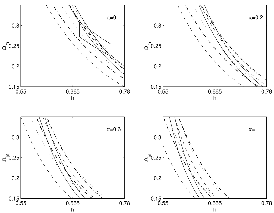
Figure 1: Contour plots of the first three Doppler peaks and first trough locations in the $(\Omega_{m},h)$ plane for GCG model, with $n_{s}=0.97$, for different values of $\alpha$. Full, dashed, dot-dashed and dotted contours correspond to observational bounds on, respectively, $\ell_{p_{1}}$, $\ell_{p_{2}}$, $\ell_{p_{3}}$ and $\ell_{d_{1}}$, see Eqs. (15) and (16). The box on the $\alpha=0$ plot (corresponds to $\Lambda$CDM model) indicates the bounds on $h$ and $\Omega_{m}h^{2}$ from a combination of WMAP and other experiments, Eq. (18).

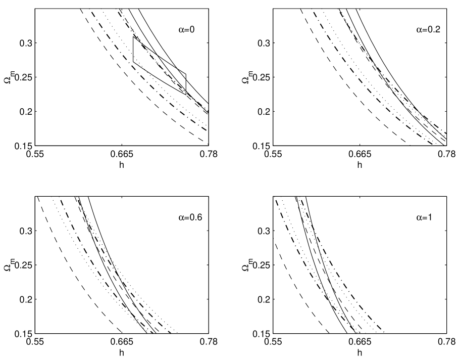
Figure 3: As for Fig. 1 but with $n_{s}=1.03$.

From the computation of the acoustic scale, Eq. (12), the equation for the shift of the peaks, Eq. (6), and the fitting formulae given in the Appendix, we look for the combination of GCG model parameters that is consistent with observational bounds. Our results are shown in Figures 1 - 4, where have assumed that $\omega_{b}=0.0224$ and used the fact that $A_{s}$ and $\Omega_{m}$ are related by

$$A_{s}={1-\Omega_{m}-\Omega_{r}\over 1-\Omega_{b}-\Omega_{r}}~{}~{}.$$ (17)

which is obtained by noting that for $\alpha=0$ the model is just the $\Lambda$CDM model; thus, one should identify the Chaplygin gas parameters with the usual density parameters when substituing $\alpha=0$ in Eq. (8) (for the present, $a_{0}=1$), taking into account that $\Omega_{m}=\Omega_{b}+\Omega_{CDM}$.

In Fig. 1, we plot contours in the $(h,\Omega_{m})$ plane corresponding to the bounds on the first three peaks and first trough of the CMBR power spectrum, Eqs. (15) - (16), for $n_{s}=0.97$ and different values of $\alpha$. The box on the $\alpha=0$ ($\Lambda$CDM model) plot corresponds to the bounds on $h$ and $\omega_{m}$ arising from the combination of WMAP data with other CMB experiments (ACBAR and CBI), 2dFGRS measurements and Lyman $\alpha$ forest data [25]:

$$h=0.71^{+0.04}_{-0.03}~{},~{}~{}~{}\omega_{m}=0.135^{+0.008}_{-0.009}~{}.$$ (18)

Notice that the above bound on $h$ is slightly more restrictive than the bound obtained from WMAP data alone [25]

$$h=0.72\pm 0.05~{}.$$ (19)

Figures 2 and 3 show the same contours but for $n_{s}=1$ and $1.03$, respectively. In Figs. 4 and 5, contours are shown in the $(A_{s},\alpha)$ plane for $h=0.71$ and $h=0.6$.

3 Discussion and Conclusions

In this work we have shown that current bounds on the location of the first few peaks and troughs in the CMBR power spectrum, as determined from WMAP and BOOMERanG data, allow constraining a sizeable portion of the parameter space of the GCG model. Our results indicate that WMAP bounds imply that the Chaplygin gas model ($\alpha=1$ case) is ruled out and so are models with $\alpha>0.6$. For low values of $n_{s}$, $\alpha=0.6$ is also ruled out. However, for $n_{s}>0.97$, $\alpha=0.6$ becomes increasingly compatible with data. Hence, one can safely state that models with $\alpha\leq 0.2$ are always consistent.

Our analysis shows that results depend strongly on the Hubble parameter and since WMAP’s bound on this quantity was obtained for $\Lambda$CDM models and, on the other hand, there are recent determinations of the Hubble constant, combining Sunayev-Zeldovich and X-ray flux measurements of clusters of galaxies, that give much lower values of $H_{0}$, namely [27]

$$H_{0}=60\pm 4^{+13}_{-18}~{}\mbox{km/s/Mpc}~{},$$ (20)

and [28]

$$H_{0}=66^{+14}_{-11}\pm 15~{}\mbox{km/s/Mpc}~{},$$ (21)

it is relevant to examine the implications, in particular regarding the exclusion of the Chaplygin gas model, of relaxing the bound (19) and allow for lower values of $h$. Figures 4 and 5 show that, for $h=0.71$ (the central value for WMAP’s bound on $h$), $\alpha=1$ is not allowed for any combination of parameters; however, for $h=0.6$ (slightly below WMAP’s preferred range), $\alpha=1$ is allowed provided $n_{s}$ is around $1$. In fact, a deeper analysis shows that, in order for the Chaplygin gas model to become consistent with peak and dip locations of the CMBR power spectrum, it is necessary that $h\mathrel{\hbox to0.0pt{\lower 4.0pt\hbox{\hskip 1.0pt$\sim$}\hss}\raise 1.0pt\hbox{$<$}}0.65$ and $n_{s}\approx 1$.

These results are compatible with the ones found in Ref. [17] using bounds on the third peak from BOMERanG and the first peak from Archeops [29] data as well as bounds from SNe Ia and distant quasar sources, namely $0.2\mathrel{\hbox to0.0pt{\lower 4.0pt\hbox{\hskip 1.0pt$\sim$}\hss}\raise 1.0pt\hbox{$<$}}\alpha\mathrel{\hbox to0.0pt{\lower 4.0pt\hbox{\hskip 1.0pt$\sim$}\hss}\raise 1.0pt\hbox{$<$}}0.6$ and $0.81\mathrel{\hbox to0.0pt{\lower 4.0pt\hbox{\hskip 1.0pt$\sim$}\hss}\raise 1.0pt\hbox{$<$}}A_{s}\mathrel{\hbox to0.0pt{\lower 4.0pt\hbox{\hskip 1.0pt$\sim$}\hss}\raise 1.0pt\hbox{$<$}}0.85$. We find,in particular, that bounds from SNe Ia data, which suggest that $0.6\mathrel{\hbox to0.0pt{\lower 4.0pt\hbox{\hskip 1.0pt$\sim$}\hss}\raise 1.0pt\hbox{$<$}}A_{s}\mathrel{\hbox to0.0pt{\lower 4.0pt\hbox{\hskip 1.0pt$\sim$}\hss}\raise 1.0pt\hbox{$<$}}0.85$ [14], are consistent with our present results for $n_{s}=1$ and $h=0.71$, namely $0.78\mathrel{\hbox to0.0pt{\lower 4.0pt\hbox{\hskip 1.0pt$\sim$}\hss}\raise 1.0pt\hbox{$<$}}A_{s}\mathrel{\hbox to0.0pt{\lower 4.0pt\hbox{\hskip 1.0pt$\sim$}\hss}\raise 1.0pt\hbox{$<$}}0.87$.

Note added After we had completed this work, a related study has appeared [30] which makes a likelihood analysis based on the full WMAP CMB data set using a modified CMBfast code, with results similar to ours.

Acknowledgments

M.C.B. and O.B. acknowledge the partial support of Fundação para a Ciência e a Tecnologia (Portugal) under the grant POCTI/1999/FIS/36285. The work of A.A.S. is fully financed by the same grant.

Appendix

We reproduce here the analytic approximations for the phase shifts found in Ref. [20]. The overall phase shift is given by

$${\bar{\varphi}}=(1.466-0.466n_{s})\left[a_{1}r_{*}^{a_{2}}+0.291{\bar{\Omega}}_{ch}^{ls}\right]~{},$$ (22)

where

$$a_{1} = 0.286+0.626\omega_{b}$$

$$a_{2} = 0.1786-6.308\omega_{b}+174.9\omega_{b}^{2}-1168\omega_{b}^{3}$$ (23)

are fitting coefficients,

$${\bar{\Omega}}_{ch}^{ls}=\tau_{ls}^{-1}\int_{0}^{\tau_{ls}}\Omega_{ch}(\tau)d\tau~{},$$ (24)

and

$$r_{*}\equiv\rho_{rad}(z_{ls})/\rho_{m}(z_{ls})$$ (25)

is the ratio of radiation to matter at decoupling and $z_{ls}$ is given by Eqs. (13) - (14).

There is no relative shift of the first acoustic peak, $\delta\varphi_{1}=0$, and the relative shifts for the second and third peaks are given by

$$\delta\varphi_{2}=c_{0}-c_{1}r_{*}-c_{2}r_{*}^{-c_{3}}+0.05(n_{s}-1)~{},$$ (26)

where

$$c_{0} = -0.1+\left(0.213-0.123{\bar{\Omega}}_{ls}^{ch}\right)$$

$$\times\exp\left\{-\left(52-63.6{\bar{\Omega}}_{ls}^{ch}\right)\omega_{b}\right\},$$

$$c_{1} = 0.015+0.063\exp\left(-3500\omega_{b}^{2}\right),$$

$$c_{2} = 6\times 10^{-6}+0.137(\omega_{b}-0.07)^{2},$$

$$c_{3} = 0.8+2.3{\bar{\Omega}}_{ls}^{ch}+\left(70-126{\bar{\Omega}}_{ls}^{ch}\right)\omega_{b}~{},$$ (27)

and

$$\delta\varphi_{3}=10-d_{1}r_{*}^{d_{2}}+0.08(n_{s}-1)~{},$$ (28)

with

$$d_{1} = 9.97+\left(3.3-3{\bar{\Omega}}_{ls}^{ch}\right)\omega_{b},$$

$$d_{2} = 0.0016-0.0067{\bar{\Omega}}_{ls}^{ch}+\left(0.196-0.22{\bar{\Omega}}_{ls}^{ch}\right)\omega_{b}$$ (29)

$$+\left(2.25+2.77{\bar{\Omega}}_{ls}^{ch}\right)\times 10^{-5}\omega_{b}^{-1}.$$

The relative shift of the first trough is given by

$$\delta\varphi_{3/2}=b_{0}+b_{1}r_{*}^{1/3}\exp(b_{2}r_{*})+0.158(n_{s}-1)~{}$$ (30)

with

$$b_{0} = -0.086-0.079{\bar{\Omega}}_{ch}^{ls}-\left(2.22-18.1{\bar{\Omega}}^{ls}_{ch}\right)\omega_{b}$$

$$-\left(140+403{\bar{\Omega}}^{ls}_{ch}\right)\omega_{b}^{2}~{},$$

$$b_{1} = 0.39-0.98{\bar{\Omega}}^{ls}_{ch}-\left(18.1-29.2{\bar{\Omega}}_{ls}^{ch}\right)\omega_{b}$$ (31)

$$+440\omega_{b}^{2},$$

$$b_{2} = -0.57-3.8\exp({-2365\omega_{b}^{2}})~{},$$ (32)

Figures

Figure 2: As for Fig. 1 but with $n_{s}=1.0$.

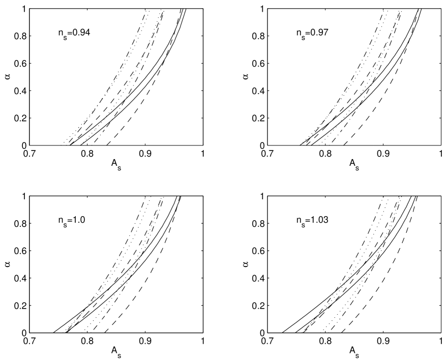
Figure 4: Contour plots of the first three Doppler peaks and first trough locations in the $(A_{s},\alpha)$ plane for GCG model, with $h=0.71$, for different values of $n_{s}$. Full, dashed, dot-dashed and dotted contours correspond to observational bounds on, respectively, $\ell_{p_{1}}$, $\ell_{p_{2}}$, $\ell_{p_{3}}$ and $\ell_{d_{1}}$, see Eqs. (15) and (16).

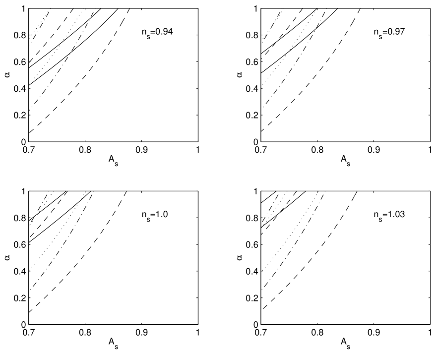
Figure 5: As for Fig. 4 but with $h=0.6$.

References

- [1] A. Kamenshchik, U. Moschella, V. Pasquier, Phys. Lett. 511 (2001) 265.
- [2] M.C. Bento, O. Bertolami, A. A. Sen, Phys. Rev. D66 (2002) 043507.
- [3] A.B. Balakin, D. Pavón, D.J. Schwarz, W. Zimdahl, astro-ph/0302150.
- [4] S.J. Perlmutter et al. (Supernova Cosmology Project), Astroph. J. 483(1997)565; Nature 391 (1998) 51; A.G. Riess et al., (Supernova Search Team) Astron. J. 116 (1998) 1009; P.M. Garnavich et al., Astroph. J. 509 (1998) 74.
- [5] N. Bilić, G.B. Tupper, R.D. Viollier, Phys. Lett. B535 (2002) 17.
- [6] J.C. Fabris, S.B.V. Gonçalves, P.E. de Souza, Gen. Relativity and Gravitation 34 (2002) 53.
- [7] M.C. Bento, O. Bertolami, Gen. Relativity and Gravitation 31 (1999) 1461; M.C. Bento, O. Bertolami, P.T. Silva, Phys. Lett. B498 (2001) 62.
- [8] M. Bronstein, Phys. Zeit. Sowejt Union 3 (1933) 73; O. Bertolami, Il Nuovo Cimento 93B (1986) 36; Fortschr. Physik 34 (1986) 829; M. Ozer, M.O. Taha, Nucl. Phys. B287 (1987) 776; B. Ratra, P.J.E. Peebles, Phys. Rev. D37 (1988) 3406; Ap. J. Lett. 325 (1988) 117; C. Wetterich, Nucl. Phys. B302 (1988) 668; R.R. Caldwell, R. Dave, P.J. Steinhardt, Phys. Rev. Lett. 80 (1998) 1582; P.G. Ferreira, M. Joyce, Phys. Rev. D58 (1998) 023503; I. Zlatev, L. Wang, P.J. Steinhardt, Phys. Rev. Lett. 82 (1999) 986; P. Binétruy, Phys. Rev. D60 (1999) 063502; J.E. Kim, JHEP 9905 (1999) 022; J.P. Uzan, Phys. Rev. D59 (1999) 123510; T. Chiba, Phys. Rev. D60 (1999) 083508; L. Amendola, Phys. Rev. D60 (1999) 043501; O. Bertolami, P.J. Martins, Phys. Rev. D61 (2000) 064007; N. Banerjee, D. Pavón, Phys. Rev. D63 (2001) 043504; Class. Quantum Gravity 18 (2001) 593; A.A. Sen, S. Sen, S. Sethi, Phys. Rev. D63 (2001) 107501; A.A. Sen, S. Sen, Mod. Phys. Lett. A16 (2001) 1303; A. Albrecht, C. Skordis, Phys. Rev. Lett. 84 (2000) 2076.
- [9] Y. Fujii, Phys. Rev. D61 (2000) 023504; A. Masiero, M. Pietroni and F. Rosati, Phys. Rev. D61 (2000) 023504; M.C. Bento, O. Bertolami, N.C. Santos, Phys. Rev. D65 (2002) 067301.
- [10] H. Sandvik, M. Tegmark, M. Zaldarriaga, I. Waga, astro-ph/0212114.
- [11] L.M.G. Beça, P.P Avelino, J.P.M. de Carvalho, C.J.A.P. Martins, astro-ph/0303564.
- [12] R. Bean, O. Doré, astro-ph/0301308.
- [13] J.C. Fabris, S.B.V. Gonçalves, P.E. de Souza, astro-ph/0207430; P.P. Avelino, L.M.G. Beça, J.P.M. de Carvalho, C.J.A.P. Martins, P. Pinto, astro-ph/0208528; A. Dev, J.S. Alcaniz, D. Jain, astro-ph/0209379; V. Gorini, A. Kamenshchik, U. Moschella, astro-ph/0209395.
- [14] M. Makler, S.Q. de Oliveira, I. Waga, astro-ph/0209486.
- [15] J.S. Alcaniz, D. Jain, A. Dev, astro-ph/0210476.
- [16] P.T. Silva, O. Bertolami, astro-ph/0303353.
- [17] M. C. Bento, O. Bertolami and A. A. Sen, Phys. Rev. D67 (2003) 063003.
- [18] D. Carturan, F. Finelli, astro-ph/0211626.
- [19] M. Doran, M. Lilley, J. Schwindt, C. Wetterich, astro-ph/0012139.
- [20] M. Doran, M. Lilley, C. Wetterich, astro-ph/0105457.
- [21] D. Di Domenico, C. Rubano, P. Scudellaro, astro-ph/0209357.
- [22] T. Barreiro, M.C. Bento, N.M.C. Santos and A.A. Sen, astro-ph/0303298.
- [23] W. Hu, M. Fukugita, M. Zaldarriaga, M. Tegmark, Astroph. J. 549 (2001) 669.
- [24] P. Bernardis et al., Astroph. J. 564 (2002) 559.
- [25] D.N. Spergel et al., astro-ph/0302207; L. Page et al., astro-ph/0302209.
- [26] W. Hu, N. Sugiyama, Astroph. J. 471 (1996) 30.
- [27] Reese et al., Astroph. J. 581 (2002) 53.
- [28] Mason et al., Astroph. J. 555 (2001) L11.
- [29] A. Benoit et al., astro-ph/0210306.
- [30] L. Amendola, F. Finelli, C. Burigana, D. Carturan, astro-ph/0304325.